
Machine Learning-Based Intelligent Prediction of Elastic Modulus of Rocks at Thar Coalfield


Abstract
:1. Introduction
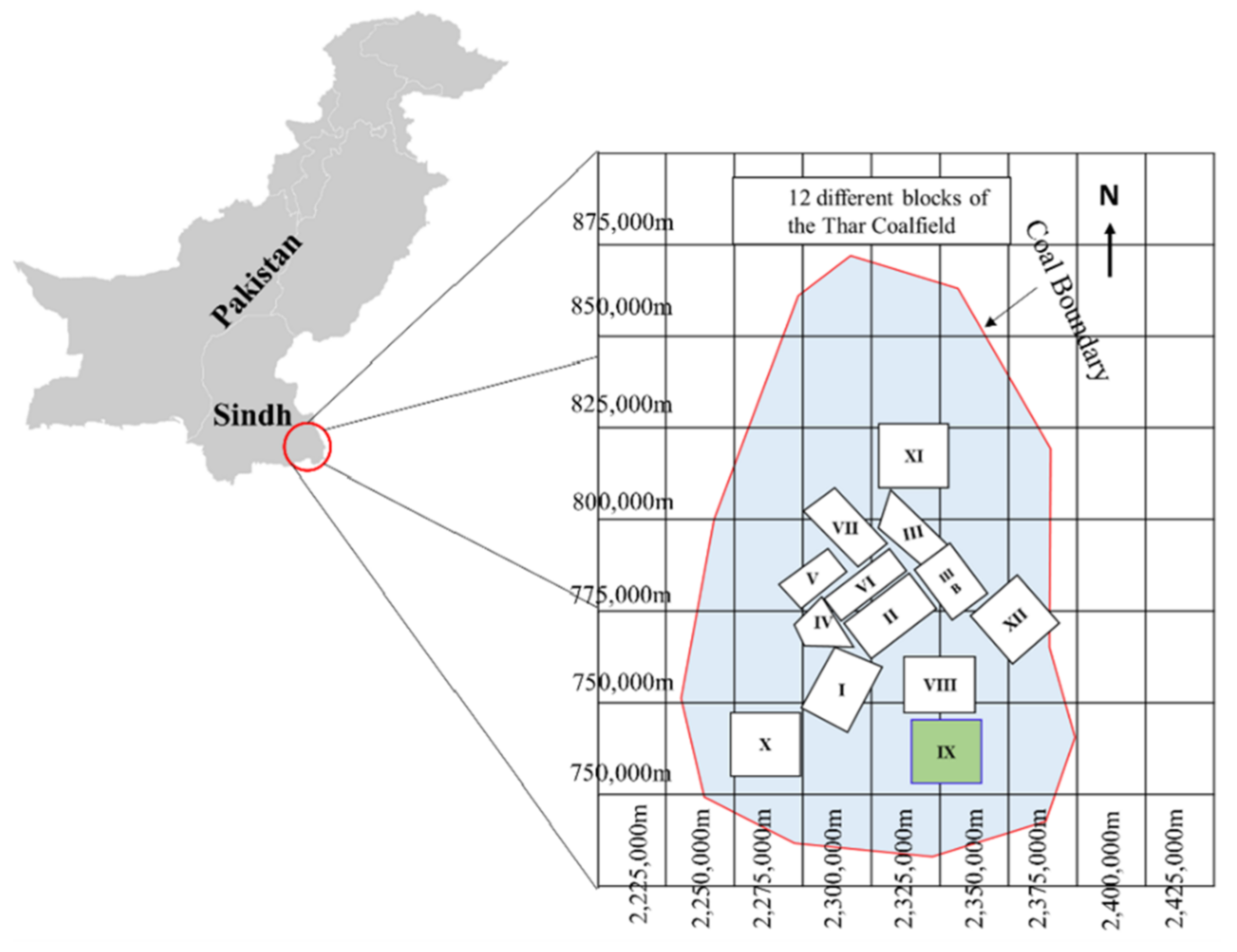
2. A Brief Summary of the Study Area
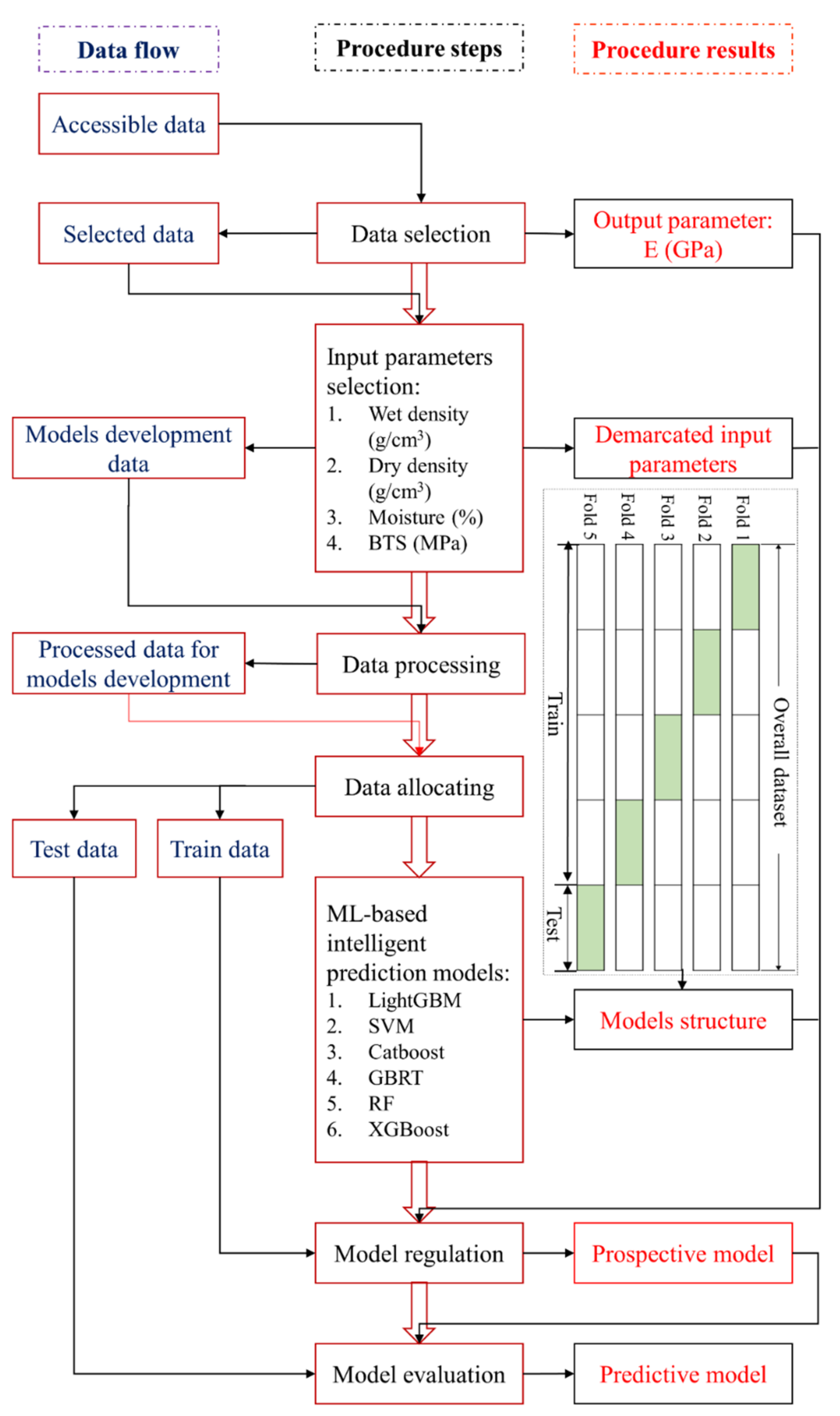
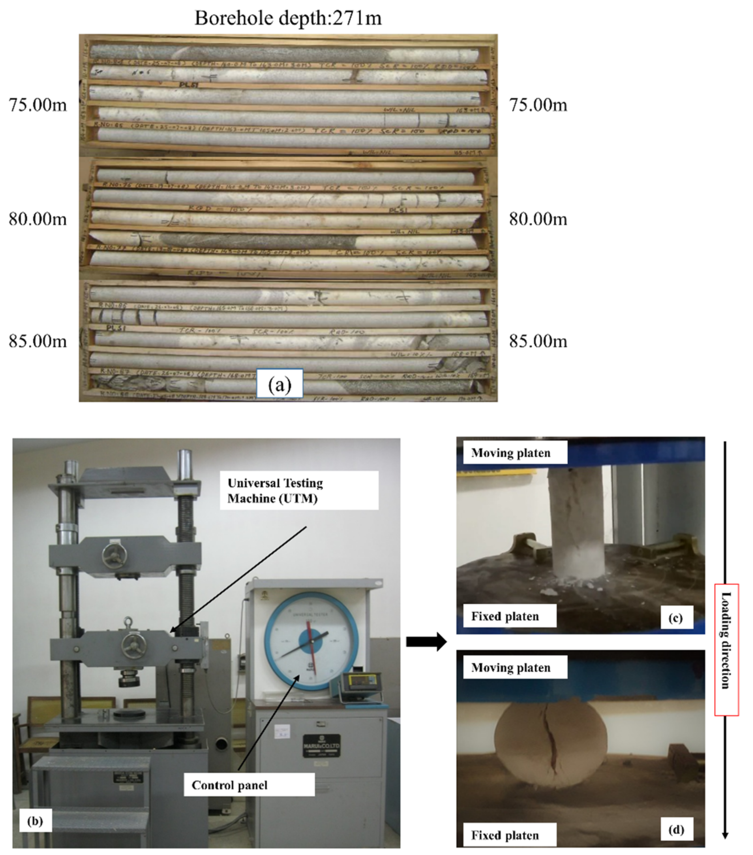
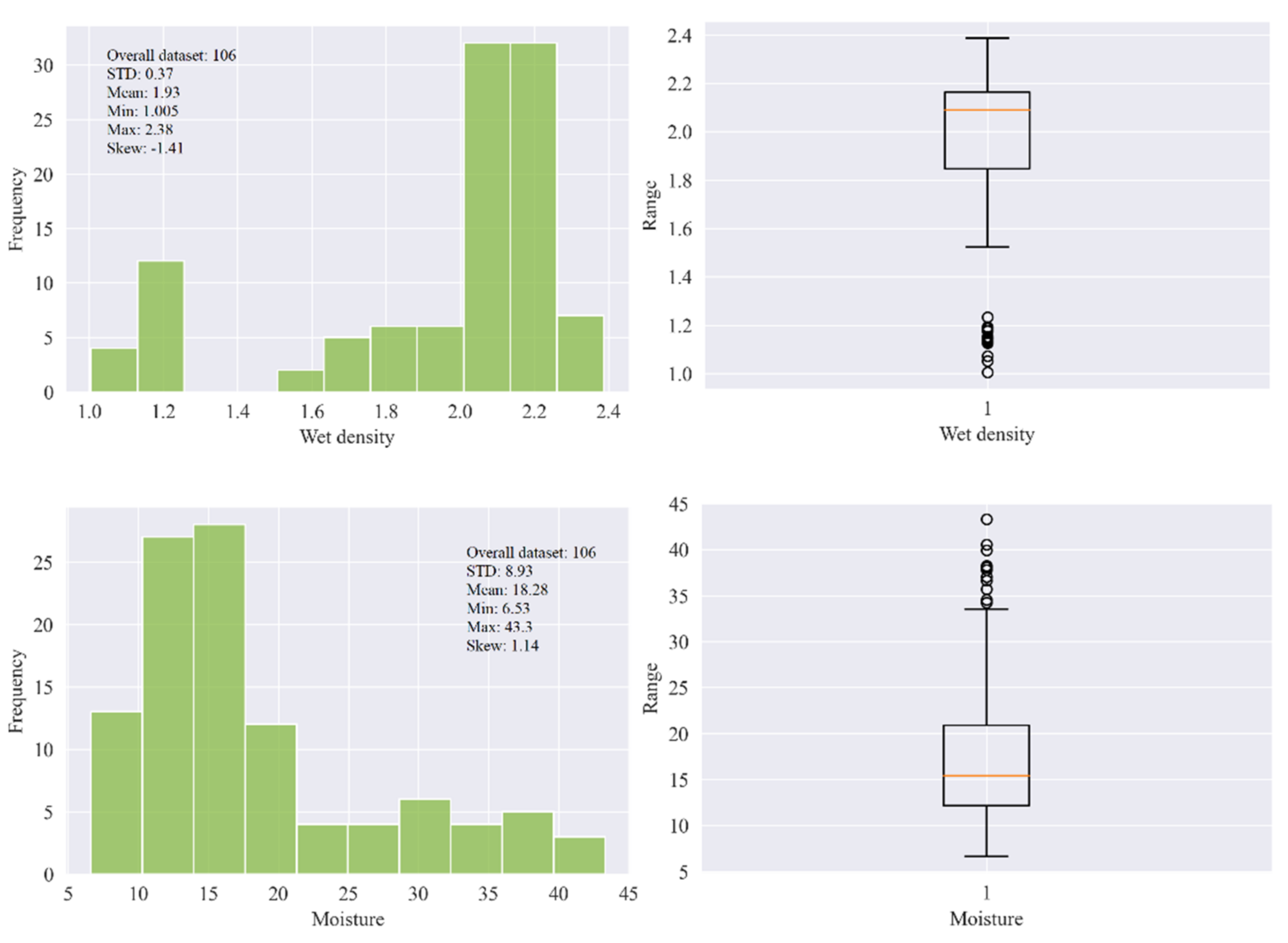
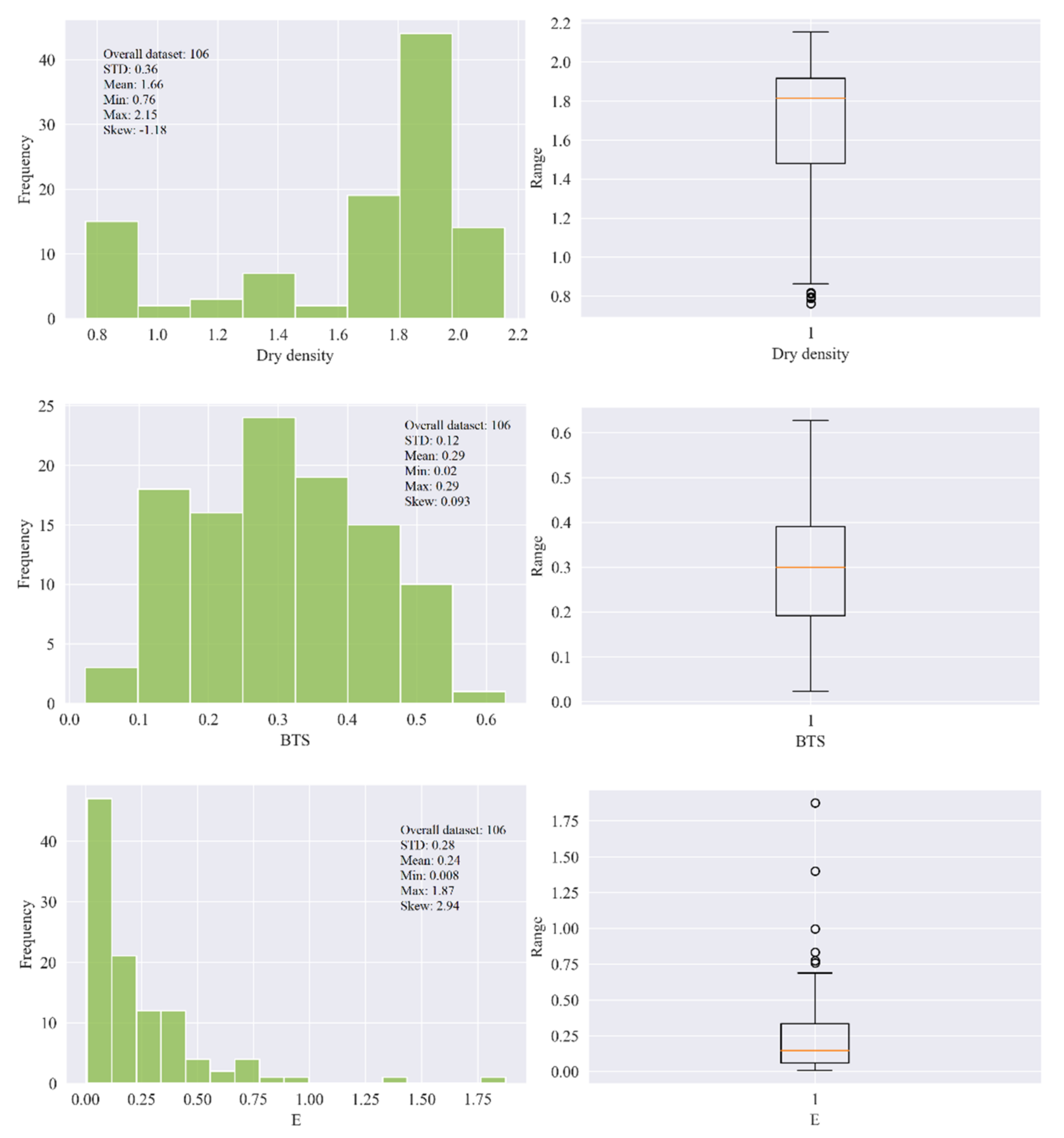
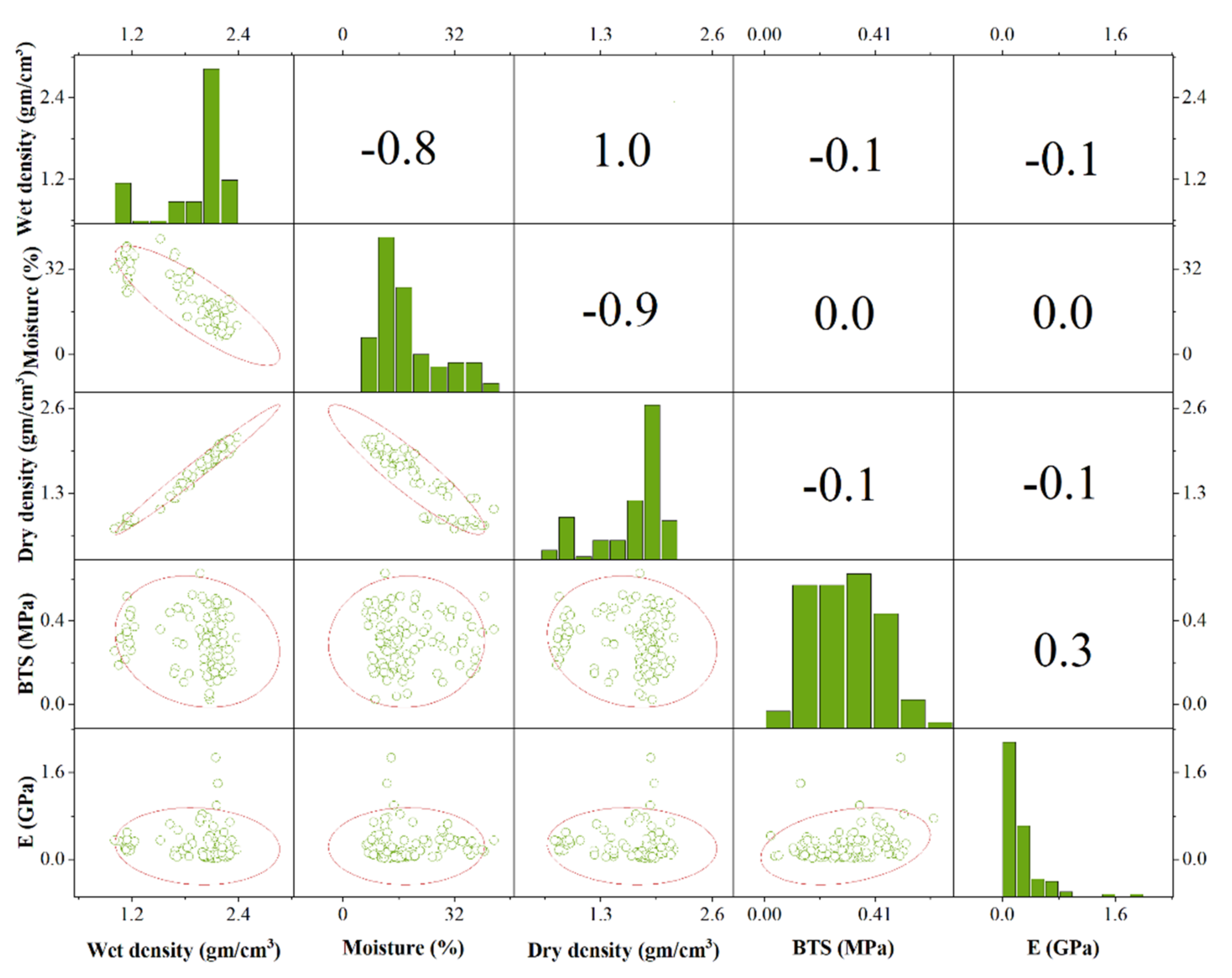
3. Data Curation
4. Developing ML-Based Intelligent Prediction Models
4.1. Light Gradient Boosting Machine
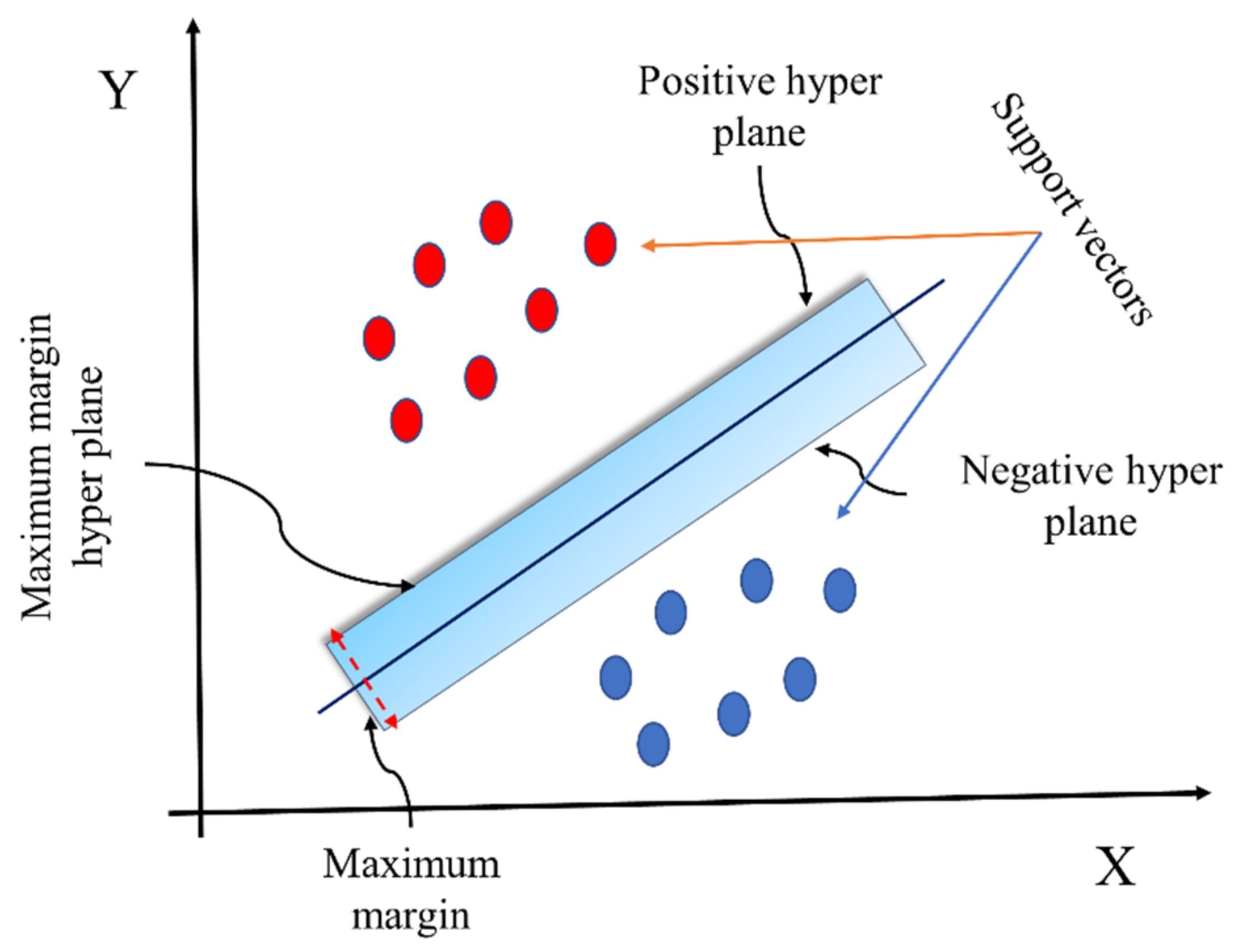
4.2. Support Vector Machine
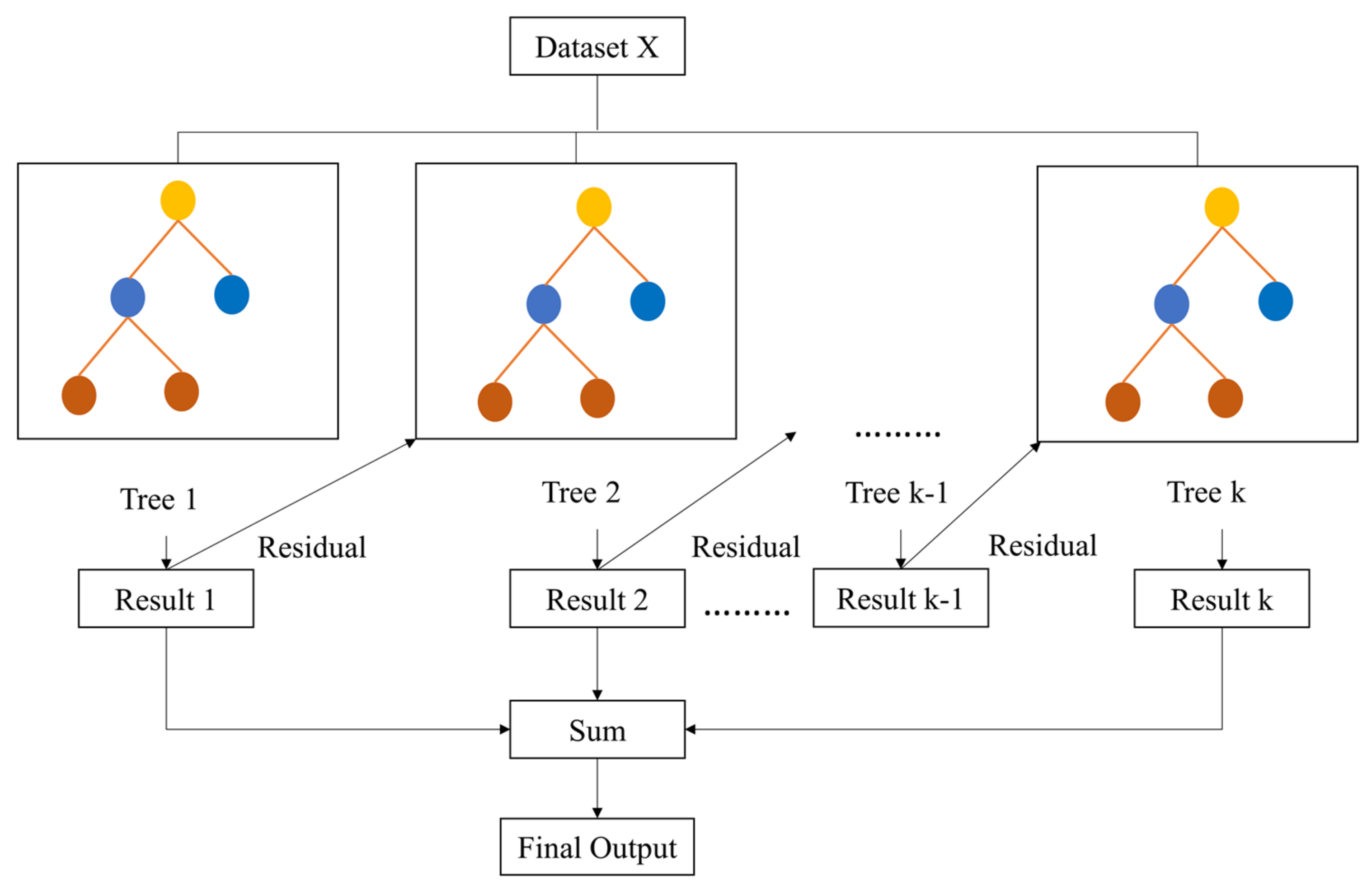
4.3. Catboost
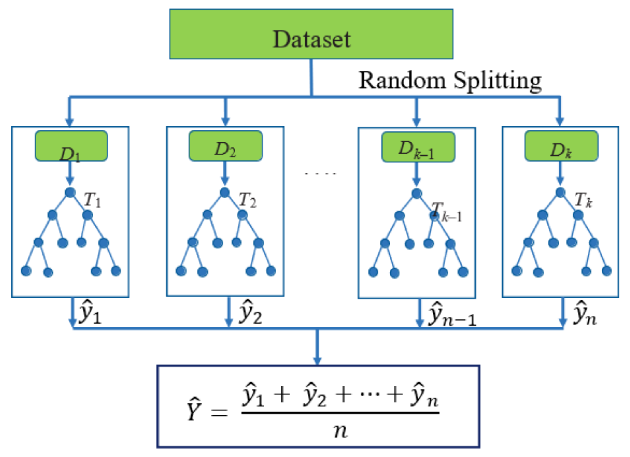
4.4. Gradient Boosted Regressor Tree
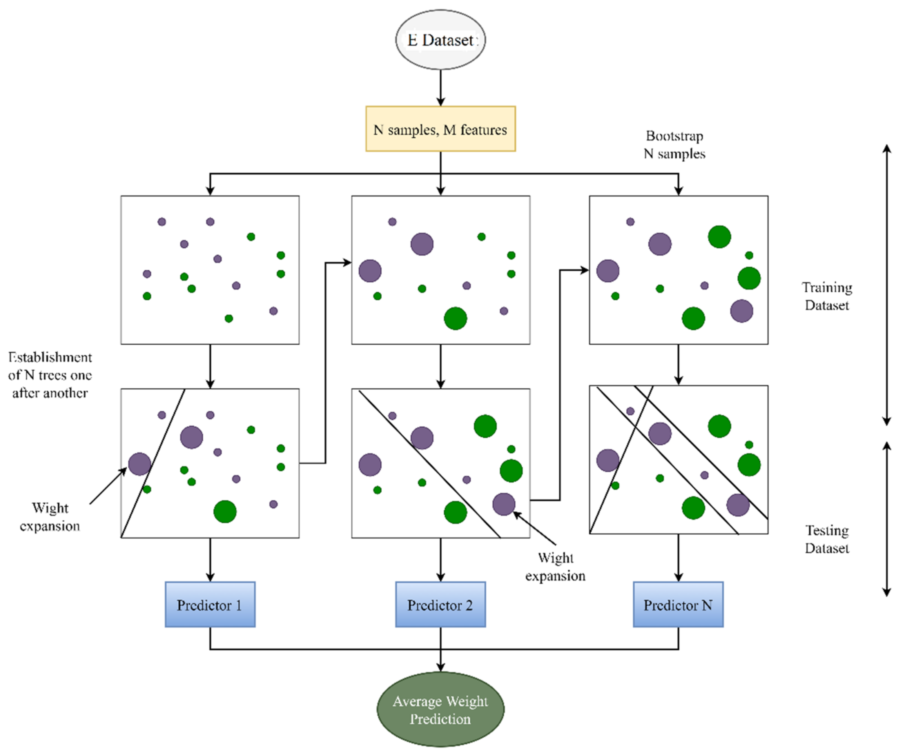
4.5. Random Forest
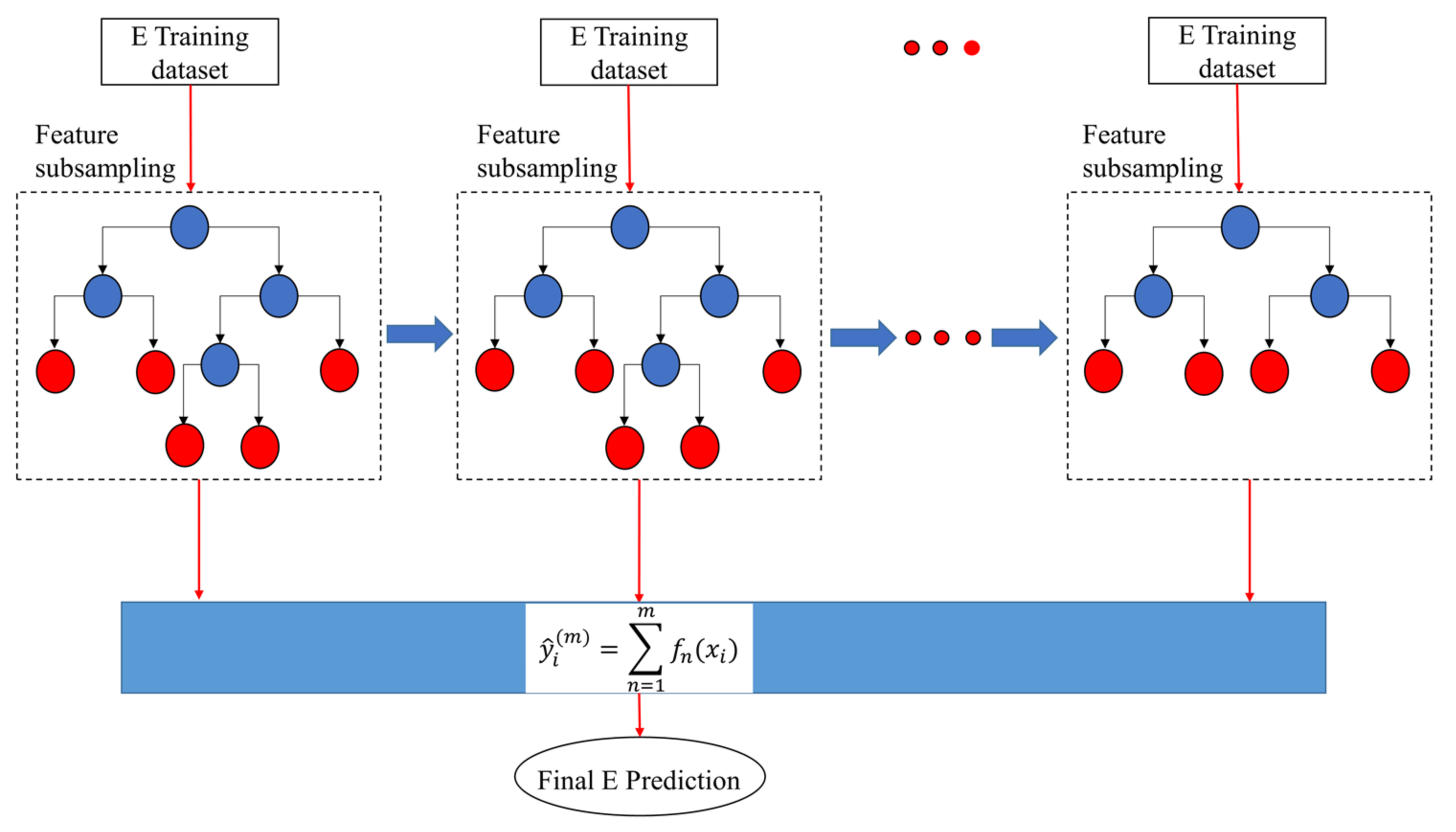
4.6. Extreme Gradient Boosting
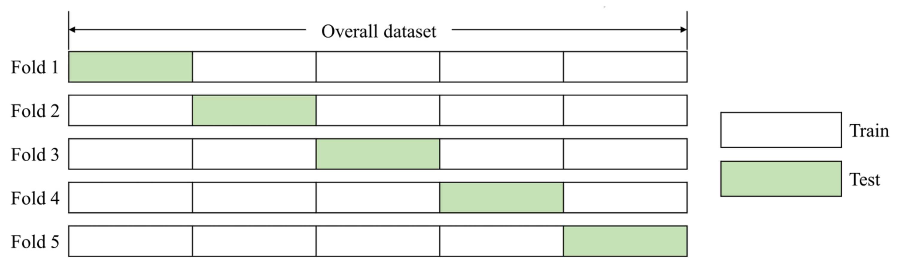
4.7. K-Fold Cross-Validation
4.8. Models Performance Evaluation
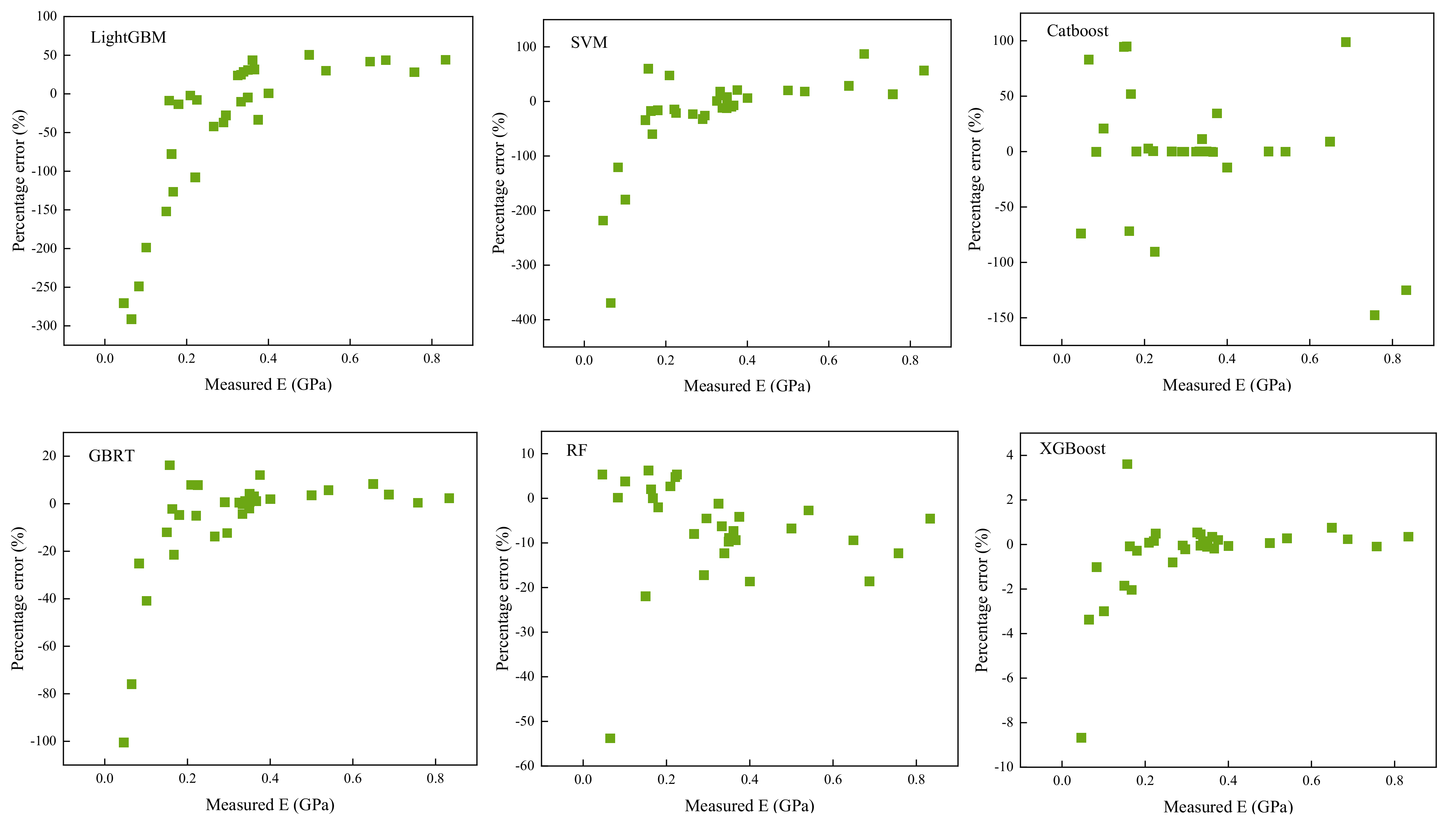
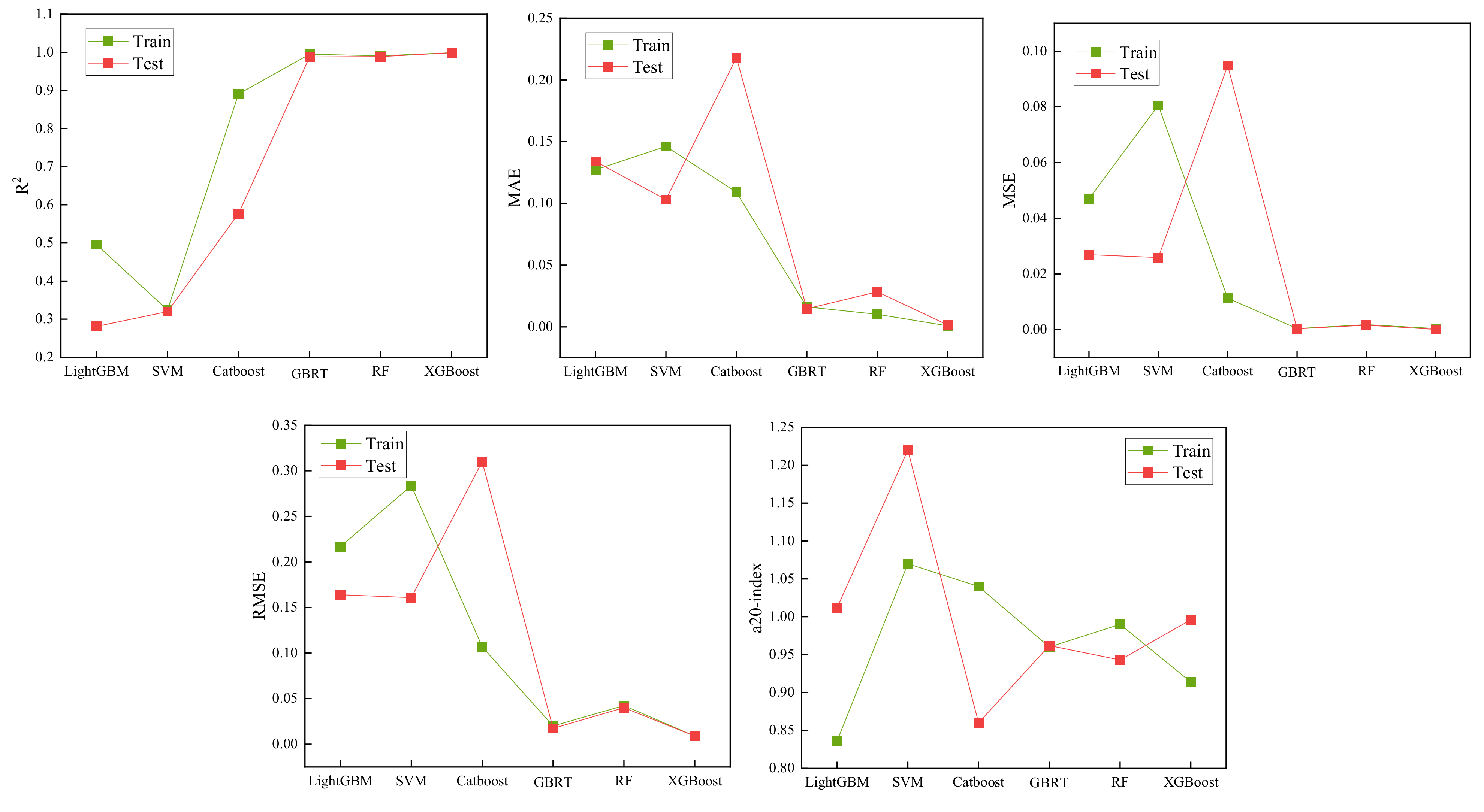
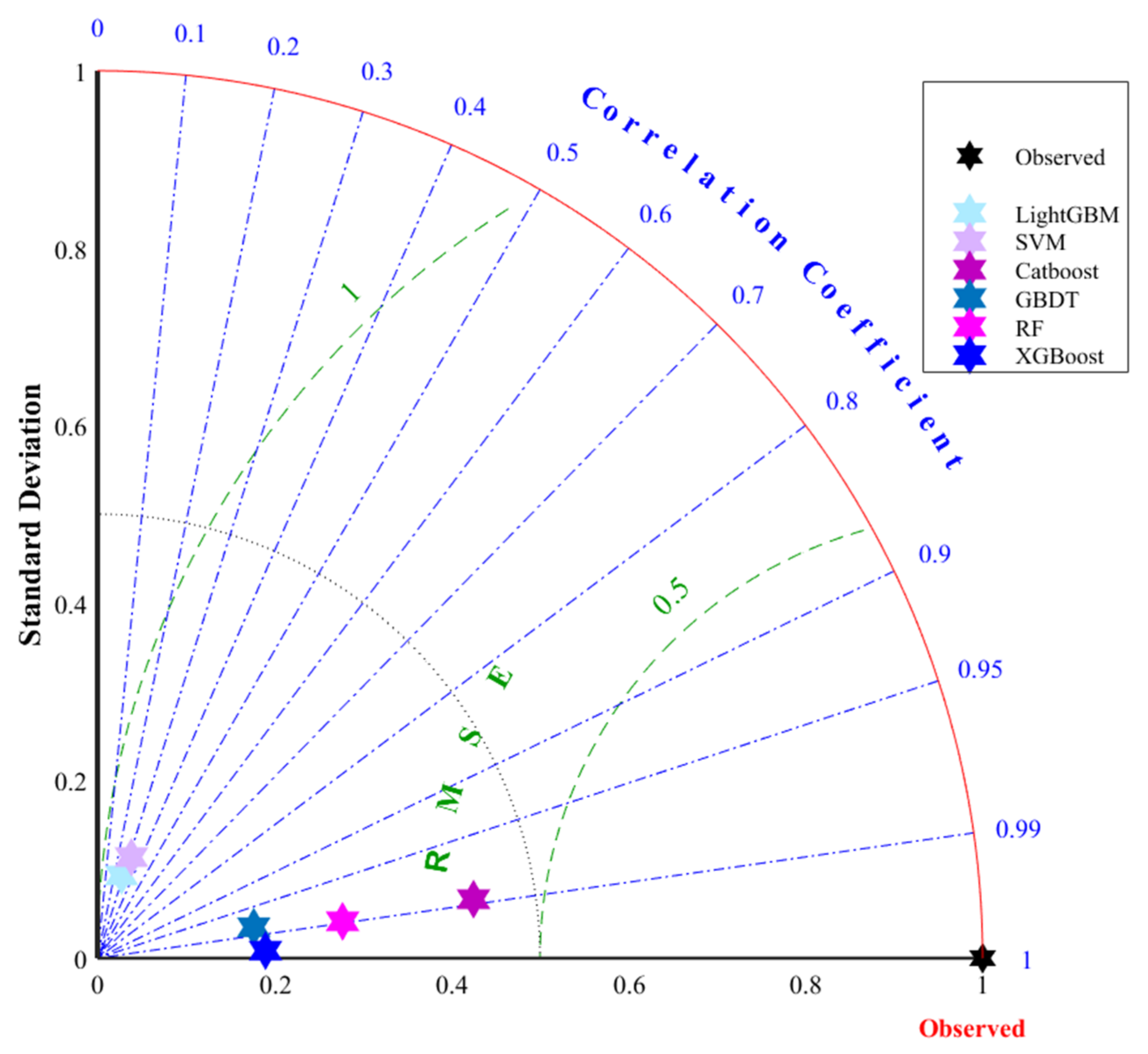
5. Analysis of Results and Discussion
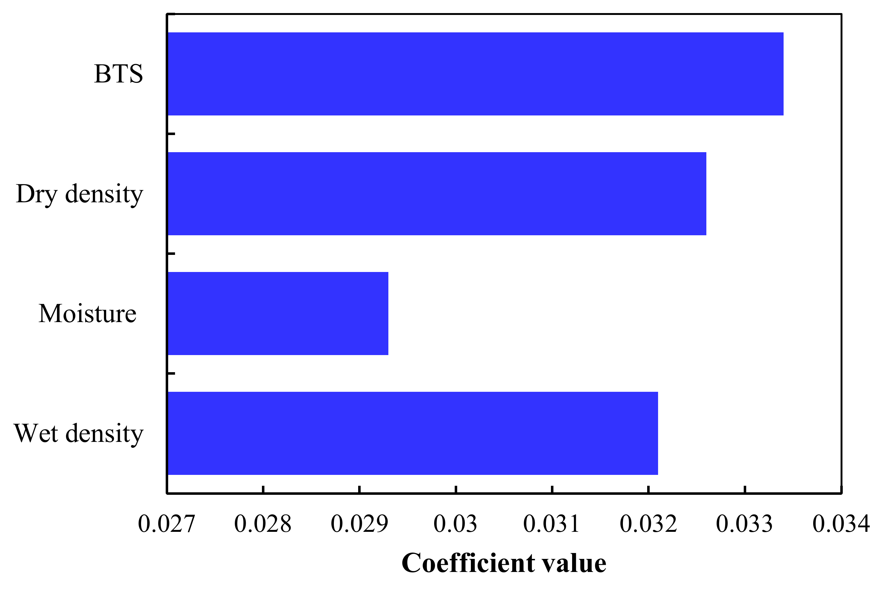
6. Sensitivity Analysis
7. Conclusions
Author Contributions
Funding
Institutional Review Board Statement
Informed Consent Statement
Data Availability Statement
Conflicts of Interest
References
- Davarpanah, M.; Somodi, G.; Kovács, L.; Vásárhelyi, B. Complex analysis of uniaxial compressive tests of the Mórágy granitic rock formation (Hungary). Stud. Geotech. Mech. 2019, 41, 21–32. [Google Scholar] [CrossRef] [Green Version]
- Xiong, L.X.; Xu, Z.Y.; Li, T.B.; Zhang, Y. Bonded-particle discrete element modeling of mechanical behaviors of interlayered rock mass under loading and unloading conditions. Geomech. Geophys. Geo-Energy Geo-Resour. 2019, 5, 1–16. [Google Scholar] [CrossRef]
- Rahimi, R.; Nygaard, R. Effect of rock strength variation on the estimated borehole breakout using shear failure criteria. Geomech. Geophys. Geo-Energy Geo-Resour. 2008, 4, 369–382. [Google Scholar] [CrossRef]
- Zhao, Y.S.; Wan, Z.J.; Feng, Z.J.; Xu, Z.H.; Liang, W.G. Evolution of mechanical properties of granite at high temperature and high pressure. Geomech. Geophys. Geo-Energy Geo-Resour. 2017, 3, 199–210. [Google Scholar] [CrossRef]
- Jing, H.; Rad, H.N.; Hasanipanah, M.; Armaghani, D.J.; Qasem, S.N. Design and implementation of a new tuned hybrid intelligent model to predict the uniaxial compressive strength of the rock using SFS-ANFIS. Eng. Comput. 2021, 37, 2717–2734. [Google Scholar] [CrossRef]
- Lindquist, E.S.; Goodman, R.E. Strength and deformation properties of a physical model melange. In Proceedings of the 1st North American Rock Mechanics Symposium, Austin, TX, USA, 1–3 June 1994; Nelson, P.P., Laubach, S.E., Eds.; Balkema: Rotterdam, The Netherlands, 1994. [Google Scholar]
- Singh, T.N.; Dubey, R.K. A study of transmission velocity of primary wave (P-Wave) in Coal Measures sandstone. J. Sci. Ind. Res. 2000, 59, 482–486. [Google Scholar]
- Tiryaki, B. Predicting intact rock strength for mechanical excavation using multivariate statistics, artificial neural networks and regression trees. Eng. Geol. 2008, 99, 51–60. [Google Scholar] [CrossRef]
- Ozcelik, Y.; Bayram, F.; Yasitli, N.E. Prediction of engineering properties of rocks from microscopic data. Arab. J. Geosci. 2013, 6, 3651–3668. [Google Scholar] [CrossRef]
- Abdi, Y.; Garavand, A.T.; Sahamieh, R.Z. Prediction of strength parameters of sedimentary rocks using artificial neural networks and regression analysis. Arab. J. Geosci. 2018, 11, 587. [Google Scholar] [CrossRef]
- Teymen, A.; Mengüç, E.C. Comparative evaluation of different statistical tools for the prediction of uniaxial compressive strength of rocks. Int. J. Min. Sci. Technol. 2020, 30, 785–797. [Google Scholar] [CrossRef]
- Li, C.; Zhou, J.; Armaghani, D.J.; Li, X. Stability analysis of underground mine hard rock pillars via combination of finite difference methods, neural networks, and Monte Carlo simulation techniques. Undergr. Space 2021, 6, 379–395. [Google Scholar] [CrossRef]
- Momeni, E.; Yarivand, A.; Dowlatshahi, M.B.; Armaghani, D.J. An efficient optimal neural network based on gravitational search algorithm in predicting the deformation of geogrid-reinforced soil structures. Transp. Geotech. 2021, 26, 100446. [Google Scholar] [CrossRef]
- Parsajoo, M.; Armaghani, D.J.; Mohammed, A.S.; Khari, M.; Jahandari, S. Tensile strength prediction of rock material using non-destructive tests: A comparative intelligent study. Transp. Geotech. 2021, 31, 100652. [Google Scholar] [CrossRef]
- Armaghani, D.J.; Harandizadeh, H.; Momeni, E.; Maizir, H.; Zhou, J. An optimized system of GMDH-ANFIS predictive model by ICA for estimating pile bearing capacity. Artif. Intell. Rev. 2021, 55, 2313–2350. [Google Scholar] [CrossRef]
- Harandizadeh, H.; Armaghani, D.J. Prediction of air-overpressure induced by blasting using an ANFIS-PNN model optimized by GA. Appl. Soft Comput. 2021, 99, 106904. [Google Scholar] [CrossRef]
- Cao, J.; Gao, J.; Rad, H.N.; Mohammed, A.S.; Hasanipanah, M.; Zhou, J. A novel systematic and evolved approach based on XGBoost-firefly algorithm to predict Young’s modulus and unconfined compressive strength of rock. Eng. Comput. 2021, 1–17. [Google Scholar] [CrossRef]
- Yang, F.; Li, Z.; Wang, Q.; Jiang, B.; Yan, B.; Zhang, P.; Xu, W.; Dong, C.; Liaw, P.K. Cluster-formula-embedded machine learning for design of multicomponent β-Ti alloys with low Young’s modulus. npj Comput. Mater. 2020, 6, 1–11. [Google Scholar] [CrossRef]
- Duan, J.; Asteris, P.G.; Nguyen, H.; Bui, X.N.; Moayedi, H. A novel artificial intelligence technique to predict compressive strength of recycled aggregate concrete using ICA-XGBoost model. Eng. Comput. 2020, 37, 3329–3346. [Google Scholar] [CrossRef]
- Pham, B.T.; Nguyen, M.D.; Nguyen-Thoi, T.; Ho, L.S.; Koopialipoor, M.; Quoc, N.K.; Armaghani, D.J.; Van Le, H. A novel approach for classification of soils based on laboratory tests using Adaboost, Tree and ANN modeling. Transp. Geotech. 2021, 27, 100508. [Google Scholar] [CrossRef]
- Asteris, P.G.; Mamou, A.; Hajihassani, M.; Hasanipanah, M.; Koopialipoor, M.; Le, T.T.; Kardani, N.; Armaghani, D.J. Soft computing based closed form equations correlating L and N-type Schmidt hammer rebound numbers of rocks. Transp. Geotech. 2021, 29, 100588. [Google Scholar] [CrossRef]
- Jordan, M.I.; Mitchell, T.M. Machine learning: Trends, perspectives, and prospects. Science 2015, 349, 255–260. [Google Scholar] [CrossRef] [PubMed]
- Waqas, U.; Ahmed, M.F. Prediction Modeling for the Estimation of Dynamic Elastic Young’s Modulus of Thermally Treated Sedimentary Rocks Using Linear–Nonlinear Regression Analysis, Regularization, and ANFIS. Rock Mech. Rock Eng. 2020, 53, 5411–5428. [Google Scholar] [CrossRef]
- Ghasemi, E.; Kalhori, H.; Bagherpour, R.; Yagiz, S. Model tree approach for predicting uniaxial compressive strength and Young’s modulus of carbonate rocks. Bull. Eng. Geol. Environ. 2018, 77, 331–343. [Google Scholar] [CrossRef]
- Shahani, N.M.; Zheng, X.; Liu, C.; Hassan, F.U.; Li, P. Developing an XGBoost Regression Model for Predicting Young’s Modulus of Intact Sedimentary Rocks for the Stability of Surface and Subsurface Structures. Front. Earth Sci. 2021, 9, 761990. [Google Scholar] [CrossRef]
- Ceryan, N. Prediction of Young’s modulus of weathered igneous rocks using GRNN, RVM, and MPMR models with a new index. J. Mt. Sci. 2021, 18, 233–251. [Google Scholar] [CrossRef]
- Umrao, R.K.; Sharma, L.K.; Singh, R.; Singh, T.N. Determination of strength and modulus of elasticity of heterogenous sedimentary rocks: An ANFIS predictive technique. Measurement 2018, 126, 194–201. [Google Scholar] [CrossRef]
- Davarpanah, S.M.; Ván, P.; Vásárhelyi, B. Investigation of the relationship between dynamic and static deformation moduli of rocks. Geomech. Geophys. Geo-Energy Geo-Resour. 2020, 6, 29. [Google Scholar] [CrossRef] [Green Version]
- Aboutaleb, S.; Behnia, M.; Bagherpour, R.; Bluekian, B. Using non-destructive tests for estimating uniaxial compressive strength and static Young’s modulus of carbonate rocks via some modeling techniques. Bull. Eng. Geol. Environ. 2018, 77, 1717–1728. [Google Scholar] [CrossRef]
- Mahmoud, A.A.; Elkatatny, S.; Ali, A.; Moussa, T. Estimation of static young’s modulus for sandstone formation using artificial neural networks. Energies 2019, 12, 2125. [Google Scholar] [CrossRef] [Green Version]
- Roy, D.G.; Singh, T.N. Regression and soft computing models to estimate young’s modulus of CO2 saturated coals. Measurement 2018, 129, 91–101. [Google Scholar]
- Armaghani, D.J.; Mohamad, E.T.; Momeni, E.; Narayanasamy, M.S. An adaptive neuro-fuzzy inference system for predicting unconfined compressive strength and Young’s modulus: A study on Main Range granite. Bull. Eng. Geol. Environ. 2015, 74, 1301–1319. [Google Scholar] [CrossRef]
- Singh, R.; Kainthola, A.; Singh, T.N. Estimation of elastic constant of rocks using an ANFIS approach. Appl. Soft Comput. 2012, 12, 40–45. [Google Scholar] [CrossRef]
- Köken, E. Assessment of Deformation Properties of Coal Measure Sandstones through Regression Analyses and Artificial Neural Networks. Arch. Min. Sci. 2021, 66, 523–542. [Google Scholar]
- Yesiloglu-Gultekin, N.; Gokceoglu, C. A Comparison Among Some Non-linear Prediction Tools on Indirect Determination of Uniaxial Compressive Strength and Modulus of Elasticity of Basalt. J. Nondestruct. Eval. 2022, 41, 10. [Google Scholar] [CrossRef]
- Awais Rashid, H.M.; Ghazzali, M.; Waqas, U.; Malik, A.A.; Abubakar, M.Z. Artificial Intelligence-Based Modeling for the Estimation of Q-Factor and Elastic Young’s Modulus of Sandstones Deteriorated by a Wetting-Drying Cyclic Process. Arch. Min. Sci. 2021, 66, 635–658. [Google Scholar]
- Matin, S.S.; Farahzadi, L.; Makaremi, S.; Chelgani, S.C.; Sattari, G. Variable selection and prediction of uniaxial compressive strength and modulus of elasticity by random forest. Appl. Soft Comput. 2018, 70, 980–987. [Google Scholar] [CrossRef]
- Yang, L.; Feng, X.; Sun, Y. Predicting the Young’s Modulus of granites using the Bayesian model selection approach. Bull. Eng. Geol. Environ. 2019, 78, 3413–3423. [Google Scholar] [CrossRef]
- Ren, Q.; Wang, G.; Li, M.; Han, S. Prediction of rock compressive strength using machine learning algorithms based on spectrum analysis of geological hammer. Geotech. Geol. Eng. 2019, 37, 475–489. [Google Scholar] [CrossRef]
- Ge, Y.; Xie, Z.; Tang, H.; Du, B.; Cao, B. Determination of the shear failure areas of rock joints using a laser scanning technique and artificial intelligence algorithms. Eng. Geol. 2021, 293, 106320. [Google Scholar] [CrossRef]
- Xu, C.; Liu, X.; Wang, E.; Wang, S. Calibration of the microparameters of rock specimens by using various machine learning algorithms. Int. J. Geomech. 2021, 21, 04021060. [Google Scholar] [CrossRef]
- Shahani, N.M.; Wan, Z.; Guichen, L.; Siddiqui, F.I.; Pathan, A.G.; Yang, P.; Liu, S. Numerical analysis of top coal recovery ratio by using discrete element method. Pak. J. Eng. Appl. Sci. 2019, 24, 26–35. [Google Scholar]
- Shahani, N.M.; Wan, Z.; Zheng, X.; Guichen, L.; Liu, C.; Siddiqui, F.I.; Bin, G. Numerical modeling of longwall top coal caving method at thar coalfield. J. Met. Mater. Miner. 2020, 30, 57–72. [Google Scholar]
- Shahani, N.M.; Kamran, M.; Zheng, X.; Liu, C.; Guo, X. Application of Gradient Boosting Machine Learning Algorithms to Predict Uniaxial Compressive Strength of Soft Sedimentary Rocks at Thar Coalfield. Adv. Civ. Eng. 2021, 2021, 2565488. [Google Scholar] [CrossRef]
- Brown, E.T. Rock Characterization Testing & Monitoring—ISRM Suggested Methods, ISRM—International Society for Rock Mechanics; Pergamon Press: London, UK, 2007; Volume 211. [Google Scholar]
- D4543-85; Standard Practices for Preparing Rock Core as Cylindrical Test Specimens and Verifying Conformance to Dimensional and Shape Tolerances. ASTM—American Society for Tenting and Materials: West Conshohocken, PA, USA, 2013.
- Ke, G.; Meng, Q.; Finley, T.; Wang, T.; Chen, W.; Ma, W.; Ye, Q.; Liu, T.Y. Lightgbm: A highly efficient gradient boosting decision tree. Adv. Neural Inf. Process. Syst. 2017, 30, 3146–3154. [Google Scholar]
- Zeng, H.; Yang, C.; Zhang, H.; Wu, Z.H.; Zhang, M.; Dai, G.J.; Babiloni, F.; Kong, W.Z. A lightGBM-based EEG analysis method for driver mental states classification. Comput. Intell. Neurosci. 2019, 2019, 3761203. [Google Scholar] [CrossRef]
- Liang, W.; Luo, S.; Zhao, G.; Wu, H. Predicting hard rock pillar stability using GBDT, XGBoost, and LightGBM algorithms. Mathematics 2020, 8, 765. [Google Scholar] [CrossRef]
- Vapnik, V.; Golowich, S.E.; Smola, A. Support vector method for function approximation, regression estimation, and signal processing. Adv. Neural Inf. Process. Syst. 1997, 9, 281–287. [Google Scholar]
- Sun, J.; Zhang, J.; Gu, Y.; Huang, Y.; Sun, Y.; Ma, G. Prediction of permeability and unconfined compressive strength of pervious concrete using evolved support vector regression. Constr. Build. Mater. 2019, 207, 440–449. [Google Scholar] [CrossRef]
- Negara, A.; Ali, S.; AlDhamen, A.; Kesserwan, H.; Jin, G. Unconfined compressive strength prediction from petrophysical properties and elemental spectroscopy using support-vector regression. In Proceedings of the SPE Kingdom of Saudi Arabia Annual Technical Symposium and Exhibition, Dammam, Saudi Arabia, 24–27 April 2017. [Google Scholar]
- Xu, C.; Amar, M.N.; Ghriga, M.A.; Ouaer, H.; Zhang, X.; Hasanipanah, M. Evolving support vector regression using Grey Wolf optimization; forecasting the geomechanical properties of rock. Eng. Comput. 2020, 1–15. [Google Scholar] [CrossRef]
- Barzegar, R.; Sattarpour, M.; Nikudel, M.R.; Moghaddam, A.A. Comparative evaluation of artificial intelligence models for prediction of uniaxial compressive strength of travertine rocks, case study: Azarshahr area, NW Iran. Model. Earth Syst. Environ. 2016, 2, 76. [Google Scholar] [CrossRef] [Green Version]
- Dong, L.; Li, X.; Xu, M.; Li, Q. Comparisons of random forest and support vector machine for predicting blasting vibration characteristic parameters. Procedia Eng. 2011, 26, 1772–1781. [Google Scholar]
- Cortes, C.; Vapnik, V. Support-vector networks. Mach. Learn. 1995, 20, 273–297. [Google Scholar] [CrossRef]
- Dorogush, A.V.; Ershov, V.; Gulin, A. CatBoost: Gradient boosting with categorical features support. arXiv 2018, arXiv:1810.11363. [Google Scholar]
- Prokhorenkova, L.; Gusev, G.; Vorobev, A.; Dorogush, A.V.; Gulin, A. CatBoost: Unbiased boosting with categorical features. Adv. Neural Inf. Process. Syst. 2018, 31, 6638–6648. [Google Scholar]
- Freund, Y.; Schapire, R.; Abe, N. A short introduction to boosting. J. Jpn. Soc. Artif. Intell. 1999, 14, 771–780. [Google Scholar]
- Schapire, R.E. The strength of weak learnability. Mach. Learn. 1990, 5, 197–227. [Google Scholar] [CrossRef] [Green Version]
- Kearns, M. Thoughts on Hypothesis Boosting. Mach. Learn. Class Proj.. 1988, pp. 1–9. Available online: https://www.cis.upenn.edu/~mkearns/papers/boostnote.pdf (accessed on 10 February 2022).
- Friedman, J.H. Greedy function approximation: A gradient boosting machine. Ann. Stat. 2001, 29, 1189–1232. [Google Scholar] [CrossRef]
- Friedman, J.; Hastie, T.; Robert, T. The elements of statistical learning. In Statistics; Springer: New York, NY, USA, 2001; Volume 1. [Google Scholar]
- Friedman, J.H. Stochastic gradient boosting. Comput. Stat. Data Anal. 2002, 38, 367–378. [Google Scholar] [CrossRef]
- Breiman, L. Random forests. Mach. Learn. 2001, 45, 5–32. [Google Scholar] [CrossRef] [Green Version]
- Yang, P.; Hwa, Y.; Zhou, B.; Zomaya, A.Y. A review of ensemble methods in bioinformatics. Curr. Bioinform. 2010, 5, 296–308. [Google Scholar] [CrossRef] [Green Version]
- Meng, Q.; Ke, G.; Wang, T.; Chen, W.; Ye, Q.; Ma, Z.M.; Liu, T.Y. A communication-efficient parallel algorithm for decision tree. Adv. Neural Inf. Process. Syst. 2016, 29, 1271–1279. [Google Scholar]
- Ranka, S.; Singh, V. Clouds: A decision tree classifier for large datasets. In Proceedings of the 4th Knowledge Discovery and Data Mining Conference, New York, NY, USA, 27–31 August 1998; pp. 2–8. [Google Scholar]
- Jin, R.; Agrawal, G. Communication and memory efficient parallel decision tree construction. In Proceedings of the 2003 SIAM International Conference on Data Mining, San Francisco, CA, USA, 1–3 May 2003; pp. 119–129. [Google Scholar]
- Bergstra, J.; Bengio, Y. Random search for hyper-parameter optimization. J. Mach. Learn. Res. 2012, 13, 281–305. [Google Scholar]
- Shahani, N.M.; Kamran, M.; Zheng, X.; Liu, C. Predictive modeling of drilling rate index using machine learning approaches: LSTM, simple RNN, and RFA. Pet. Sci. Technol. 2022, 40, 534–555. [Google Scholar] [CrossRef]
- Willmott, C.J. Some comments on the evaluation of model performance. Bull. Am. Meteorol. Soc. 1982, 63, 1309–1313. [Google Scholar] [CrossRef] [Green Version]
- Taylor, K.E. Summarizing multiple aspects of model performance in a single diagram. J. Geophys. Res. 2001, 106, 7183–7192. [Google Scholar] [CrossRef]
- Zhong, R.; Tsang, M.; Makusha, G.; Yang, B.; Chen, Z. Improving rock mechanical properties estimation using machine learning. In Proceedings of the 2021 Resource Operators Conference, Wollongong, Australia, 10–12 February 2021; University of Wollongong-Mining Engineering: Wollongong, Australia, 2021. [Google Scholar]
- Ghose, A.K.; Chakraborti, S. Empirical strength indices of Indian coals. In Proceedings of the 27th U.S. Symposium on Rock Mechanics, Tuscaloosa, AL, USA, 23–25 June 1986. [Google Scholar]
- Katz, O.; Reches, Z.; Roegiers, J.C. Evaluation of mechanical rock properties using a Schmidt Hammer. Int. J. Rock Mech. Min. Sci. 2000, 37, 723–728. [Google Scholar] [CrossRef]
- Momeni, E.; Nazir, R.; Armaghani, D.J.; Maizir, H. Prediction of pile bearing capacity using a hybrid genetic algorithm-based ANN. Measurement 2014, 57, 122–131. [Google Scholar] [CrossRef]
- Ji, X.; Liang, S.Y. Model-based sensitivity analysis of machining-induced residual stress under minimum quantity lubrication. Proc. Inst. Mech. Eng. Part B J. Eng. Manuf. 2007, 231, 1528–1541. [Google Scholar] [CrossRef]


| Model | Training | Testing | ||||||||
|---|---|---|---|---|---|---|---|---|---|---|
| R2 | MAE | MSE | RMSE | a20-Index | R2 | MAE | MSE | RMSE | a20-Index | |
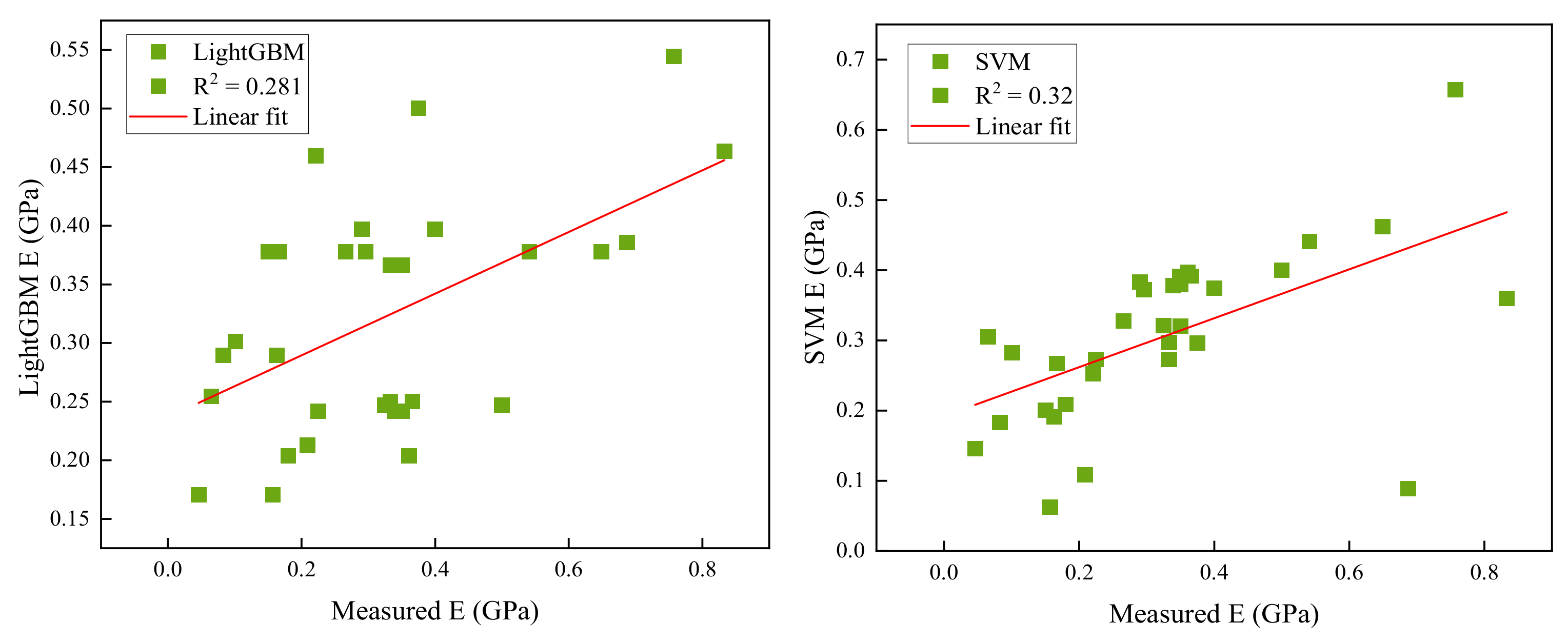
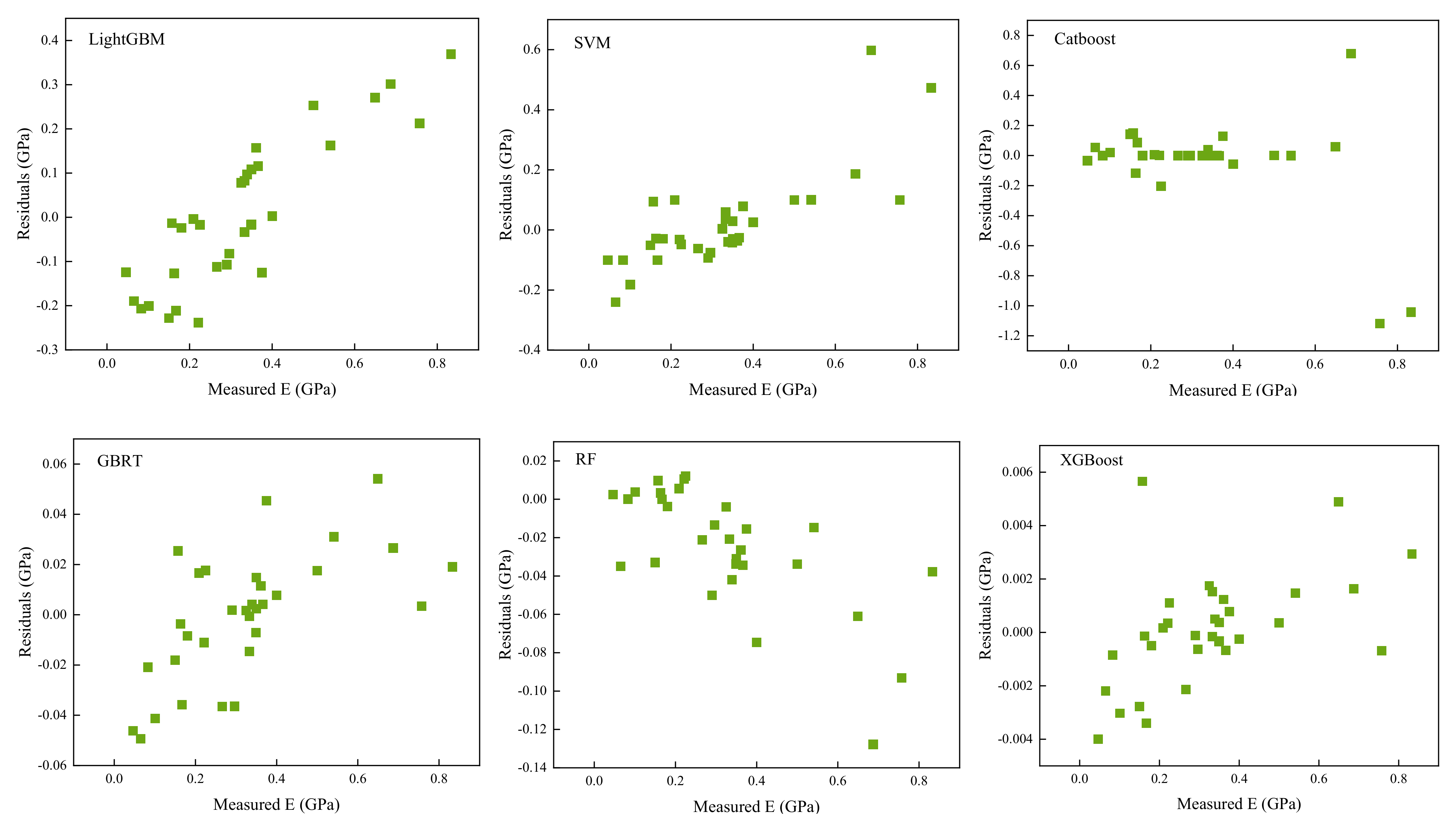
| LightGBM | 0.496 | 0.1272 | 0.0470 | 0.2168 | 0.836 | 0.281 | 0.1340 | 0.0269 | 0.1640 | 1.012 |
| SVM | 0.324 | 0.1461 | 0.0805 | 0.2837 | 1.07 | 0.32 | 0.1031 | 0.0259 | 0.1609 | 1.22 |
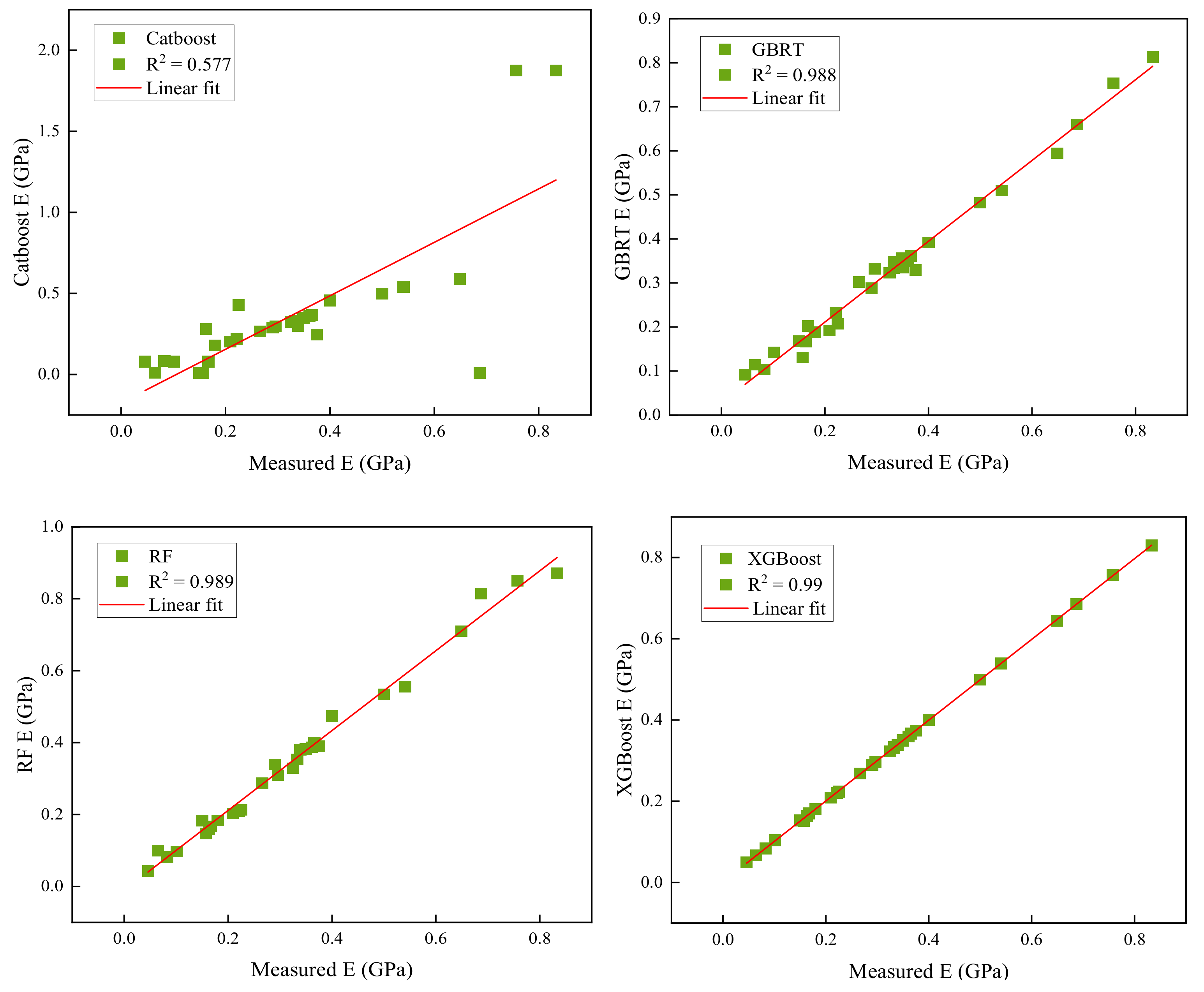
| Catboost | 0.891 | 0.1091 | 0.0113 | 0.1069 | 1.04 | 0.577 | 0.218 | 0.0948 | 0.3101 | 0.86 |
| GBRT | 0.995 | 0.0162 | 0.0004 | 0.0200 | 0.96 | 0.988 | 0.0147 | 0.0003 | 0.0173 | 0.962 |
| RF | 0.991 | 0.0102 | 0.0018 | 0.0424 | 0.99 | 0.989 | 0.0284 | 0.0016 | 0.0400 | 0.943 |
| XGBoost | 0.999 | 0.0008 | 0.0004 | 0.0089 | 0.914 | 0.999 | 0.0015 | 0.0008 | 0.0089 | 0.996 |
Publisher’s Note: MDPI stays neutral with regard to jurisdictional claims in published maps and institutional affiliations. |
© 2022 by the authors. Licensee MDPI, Basel, Switzerland. This article is an open access article distributed under the terms and conditions of the Creative Commons Attribution (CC BY) license (https://creativecommons.org/licenses/by/4.0/).
Share and Cite
Shahani, N.M.; Zheng, X.; Guo, X.; Wei, X. Machine Learning-Based Intelligent Prediction of Elastic Modulus of Rocks at Thar Coalfield. Sustainability 2022, 14, 3689. https://doi.org/10.3390/su14063689
Shahani NM, Zheng X, Guo X, Wei X. Machine Learning-Based Intelligent Prediction of Elastic Modulus of Rocks at Thar Coalfield. Sustainability. 2022; 14(6):3689. https://doi.org/10.3390/su14063689
Chicago/Turabian StyleShahani, Niaz Muhammad, Xigui Zheng, Xiaowei Guo, and Xin Wei. 2022. "Machine Learning-Based Intelligent Prediction of Elastic Modulus of Rocks at Thar Coalfield" Sustainability 14, no. 6: 3689. https://doi.org/10.3390/su14063689