Article

Random Forests Assessment of the Role of Atmospheric Circulation in PM10 in an Urban Area with Complex Topography

1
Faculty of Physics and Applied Computer Science, AGH University of Science and Technology, 30-059 Kraków, Poland
2
Institute of Meteorology and Water Management, National Research Institute, IMGW-PIB, 01-673 Warszawa, Poland
3
Institute of Geography and Spatial Management, Jagiellonian University, 30-387 Kraków, Poland
*
Author to whom correspondence should be addressed.
Sustainability 2022, 14(6), 3388; https://doi.org/10.3390/su14063388
Submission received: 20 January 2022 / Revised: 8 March 2022 / Accepted: 10 March 2022 / Published: 14 March 2022
(This article belongs to the Collection Air Pollution Control and Sustainable Development)

Abstract

:
This study presents the assessment of the quantitative influence of atmospheric circulation on the pollutant concentration in the area of Kraków, Southern Poland, for the period 2000–2020. The research has been realized with the application of different statistical parameters, synoptic meteorology tools, the Random Forests machine learning method, and multilinear regression analyses. Another aim of the research was to evaluate the types of atmospheric circulation classification methods used in studies on air pollution dispersion and to assess the possibility of their application in air quality management, including short-term PM10 daily forecasts. During the period analyzed, a significant decreasing trend of pollutants’ concentrations and varying atmospheric circulation conditions was observed. To understand the relation between PM10 concentration and meteorological conditions and their significance, the Random Forests algorithm was applied. Observations from meteorological stations, air quality measurements and ERA-5 reanalysis were used. The meteorological database was used as an input to models that were trained to predict daily PM10 concentration and its day-to-day changes. This study made it possible to distinguish the dominant circulation types with the highest probability of occurrence of poor air quality or a significant improvement in air quality conditions. Apart from the parameters whose significant influence on air quality is well established (air temperature and wind speed at the ground and air temperature gradient), the key factor was also the gradient of relative air humidity and wind shear in the lowest troposphere. Partial dependence calculated with the use of the Random Forests model made it possible to better analyze the impact of individual meteorological parameters on the PM10 daily concentration. The analysis has shown that, for areas with a diversified topography, it is crucial to use the variability of the atmospheric circulation during the day to better forecast air quality.

1. Introduction

The abundant air pollution with particulate matter (PM) is a serious environmental and social problem in many regions all over the world [1,2,3,4]. Exposure to ambient PM concentration with a diameter below 10 μm (PM10) increases the possibility of preterm birth [5], deaths from respiratory disease [6] and also causes lung irritation, cellular damage, coughing asthma, and cardiovascular diseases [7]. High PM concentrations in urbanized areas are the consequence of the interaction of many factors, including anthropogenic and natural sources of air pollution, chemical and physical reactions between primary and secondary pollutants, and dispersion conditions determined by atmospheric circulation types, meteorological conditions, and meso- and microclimatic features of the analyzed area [1,8,9]. Numerous studies confirm that atmospheric circulation is an important factor determining the level of air pollution in the lower troposphere, especially in urbanized and industrial areas, which are characterized by elevated pollution emissions [3,10,11,12,13]. The atmospheric circulation processes contribute not only to the dispersion of pollution but also to its transport over great distances from emission sources [14]. Previous research indicated that the duration of air pollution episodes is mainly influenced by the processes of atmospheric blocking and atmospheric stagnation, which contribute to the accumulation of pollutants near the ground, especially during wintertime periods [3,15,16]. Analyses of future climate change indicate that the occurrence of an increase in air stagnation cases is expected [17,18]. Studies performed for Thessaloniki showed that smog episodes can also occur often under weak flow conditions, with warm air advection, as a consequence of stabilization of the lower troposphere and limited vertical mixing [19]. A similar effect of reducing the available mixing volume caused by warm air advection occurs often in mountain valleys and is linked to foehn occurrence [20,21]. It is worth mentioning that similar local weather conditions can occur under very different rearrangements of the large-scale flow; therefore, there is a need to study the relations between unfavorable local pollutant dispersion conditions and large-scale atmospheric circulation, with the impact of particular environmental features.
The problem of the increased PM10 concentration level in the European Union is common for all the nations which are members; in 2018, the daily PM10 concentration limit (50 μg⋅m−3) was exceeded in numerous cities in Poland, Bulgaria, the Czech Republic, Croatia, Hungary, Italy and Slovenia [22]. In Poland, poor air quality is a problem, especially in southern regions, both in urban agglomerations and many small localities, where the highest number of days with exceedance of the daily limit of PM10 concentration on the national scale is noted [23]. The problem of air quality in Southern Poland also concerns the area of Kraków, the second largest city in Poland in terms of the number of inhabitants, where air pollution has been a serious and unsolved environmental and social problem for several decades [24,25,26]. In the Małopolska region, where Kraków is located, the main source of PM10 is the emission from the municipal and housing sector (78.9% of the annual emission), from transportation (5%), and from industry (7.8%). During recent decades, there have been many actions aimed to reduce local emissions of PM10 and SO2 from different sectors. Those actions include liquidation of solid fuel boilers, thermal modernization of buildings, installation of renewable energy sources, modernization of public transport and heating networks or the expansion of bicycle routes. As a result, the air quality in the city has gradually improved, although the PM10 daily limits are still exceeded during the cold seasons [23]. In addition, on 1 September 2019, the prohibition of solid fuels usage in individual heating devices in Kraków was introduced, which could partially contribute to the reduction of PM concentration level during the cold season. The atmospheric circulation conditions play a crucial role in determining the air quality in the city, as it is located in the Wisła River valley, in an area of very diversified relief. The properties of planetary boundary layer (PBL) are strongly modified both by the relief and the synoptic situation, and so are the air pollution’s dispersion conditions which in turn affect the concentration of pollutants. Studies of fog occurrence for Kraków city for the period from 1965 to 2015 indicated that fog occurred usually on days with non-advective anticyclonic types Ca and Ka or cyclonic and anticyclonic advection from sector S-SW (types SWa and Sc) according to Niedźwiedź classification [27]. This indicated that the majority of winter fogs at Kraków might be related to air pollution from heating during frosty anticyclonic winter weather. Research of long-term variability of the cloud for Kraków has shown that the greatest cloudiness and one of the smallest variabilities are associated with cyclonic situations involving northerly and northeasterly advection. The relationships between the cloudiness and atmospheric circulations were stronger during the cold half of the year than during the warm half, when the radiation factor plays a major role [28]. One of the situations when the influence of atmospheric circulation on air pollution dispersion is well visible is the occurrence of foehn winds, which can worsen or improve the air quality in the city [21].
High weather variability in Poland is associated with frequent movement of low and high-pressure systems [29]. Studies of circulation types for Kraków in the 20th century were summarized by Z. Ustrnul [30]. Significant variation in the annual incidence of individual circulation types according to the Niedźwiedź classification was found; the most frequent were anticyclonic non-directional types (high-pressure center and anticyclonic wedge or ridge); they constituted 15% of all cases during the year. The second most common types were those with the advection of air masses from the western sector (SW-W-NW) (both during anticyclonic and cyclonic situations), with the frequency reaching a total of 40% during the year. The least frequent were the cyclonic types, with the advection of air from the North and the eastern sector. In the individual seasons (from spring to winter), there was quite large variability in dominant circulation types. A slight positive trend was observed for circulation types with air advection from the West. In the 20th century, circulation types were characterized by high inter-annual frequency variability and the absence of distinct, characteristic periods, with the prevalence of certain types.
Assessment of the role of atmospheric circulation on PM10 concentration level during a particular period is highly challenging because many factors including emission level, changeable weather conditions, microclimatic features and chemical and physical processes affect the air quality levels.
Recently, there has been a growing interest in the application of machine learning techniques in statistical analysis [31,32] and forecasting air quality over the wide temporal and spatial scale [33,34]. The most commonly used machine learning tools include Artificial Neural Network [35], Deep Neural Network, Extreme-Gradient Boosting [36] and Random Forests [33]. Machine learning techniques have been successfully applied to assess population exposure to poor air quality in metropolitan areas [33], downscaling of air pollutants at a higher resolution [37], and also meteorological normalization used in air quality trend analysis [31]. Random Forests, which is a machine learning method based on constructing decision trees, is widely used for regression and classification. One of the main advantages of this method, besides its being accurate and straightforward in implementation, is the simple and intuitive way of accessing variables that are important in the process of training the model in complex and nonlinear problems. The research was undertaken in order to assess the quantitative influence of atmospheric circulation on the pollutant concentration in the area of Kraków, and to compare the results for the study period mentioned with the research from earlier decades. The research was also aimed to evaluate two main groups of the classification methods of atmospheric circulation types’ used in studies on air pollution dispersion (described in Section 2.5), and to assess the possibility of their application in air quality management. In our study, we were focused more on the interpretation of the importance of variables by the Random Forests technique than predictions of the model itself. Kraków is an adequate study area for such considerations as, on one hand, it is located in diversified environmental conditions, and on the other hand, relatively long series of air quality measurements are available. Two different classifications of atmospheric circulation were used in the present study: a manual classification by Niedźwiedź [29] and an automatic classification by Lityński [38,39]; those two different classifications were used with the aim of minimizing the risk of misinterpretation of the results, and both classification methods were widely used by different groups of researchers in studies of atmospheric types over Central Europe [14,40,41]. Previous studies concerning the influence of atmospheric circulation on air quality in Krakow, with the application of Niedźwiedź classification, have been summarized in the monograph by J. Godłowska [42]. The research indicated that during air masses advection from S-SW sector and non-directional circulation types (high-pressure center and anticyclonic wedge or ridge), wind speed near the ground was reduced, which in consequence could lead to the occurrence of a high-level PM10 concentration during the cold season. Studies of atmospheric stability in Kraków using SODAR for the period 1994–1999 showed that, for types with air masses advection from a direction between 135° and 225°, the anticyclonic wedge and the high-pressure center, the duration of elevated thermal inversions in the cold season was the longest.
Understanding the relationship between the pollutants’ concentration and the atmospheric circulation, at the synoptic and local scale, is crucial for forecasting air pollution episodes and minimizing the negative impact of air pollution on the health of city residents and on the condition of the natural environment.

2. Material and Methods
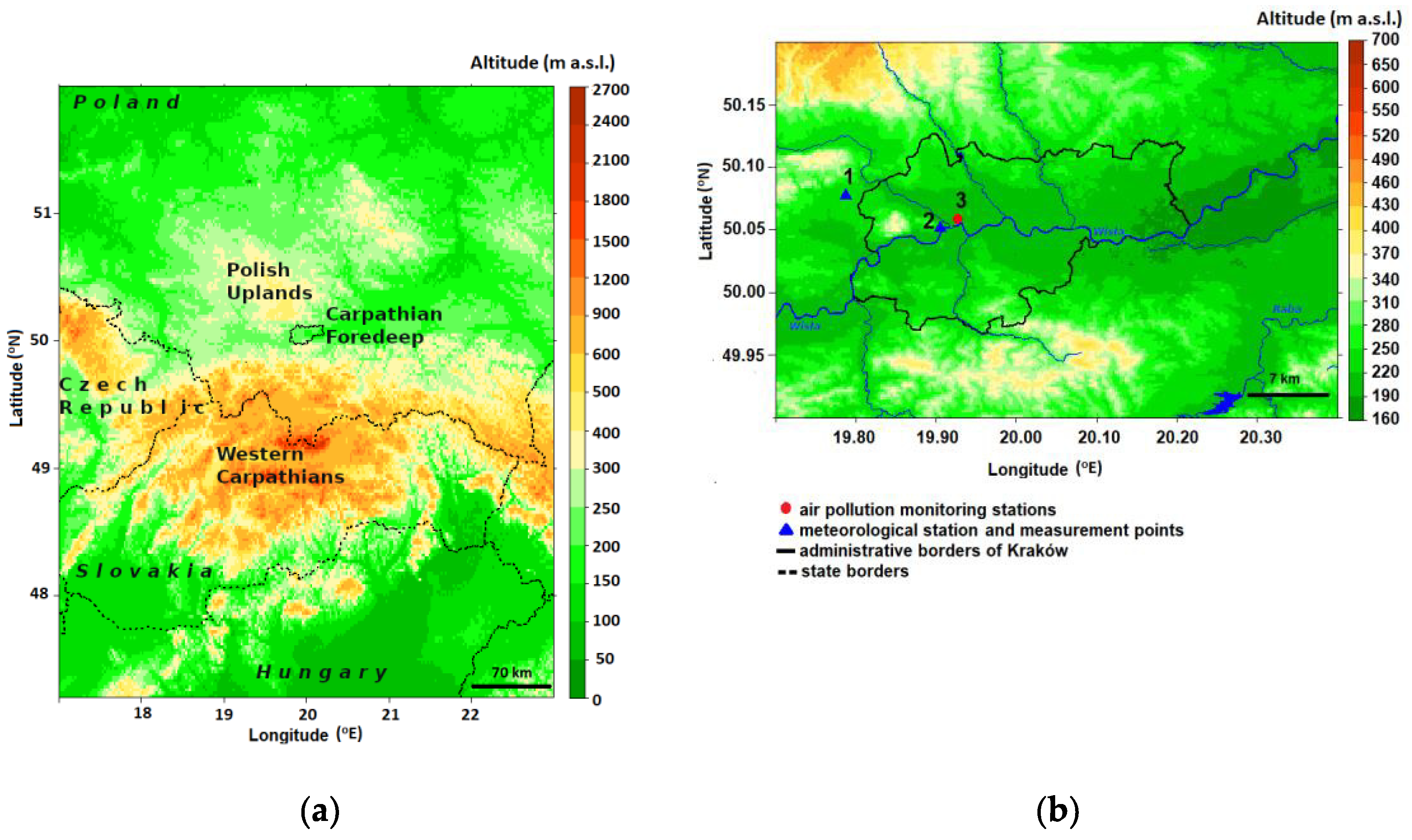
Data used in the present study come from different sources and cover the period October 2000–September 2020 (additionally, the period October 2021–December 2021 was selected for operational tests of the predictive model). Data analyses were realized for two sub-periods: cold half-year (October–March) and warm half-year (April–September), owing to significant differences in air pollution emissions and concentrations, which have been observed in Kraków in those sub-periods. First, data sets are described, and their basic statistical features are shown, then the methods combining data from different data sets are presented. Air quality in Kraków was characterized with data on PM10 as the allowed concentrations of that pollutant are exceeded much more frequently than the concentrations of other pollutants. The authors are aware that the division of the year proposed above is only one of the options available, as, in particular years, the frequency of circulation types and meteorological conditions may change significantly; however, such a division was also used in other climatological studies [43,44].

2.1. Study Area

Kraków is the second largest city in Poland, located in the Małopolska (Lesser Poland) region, with an area of 326.8 km2 and the number of inhabitants reaching almost 800,000 [45]. The Kraków agglomeration consists of the city itself and the highly populated towns and villages which surround it, and the total number of inhabitants is estimated to exceed 1 million. The city’s area belongs to three different geographical regions and geological structures presented at Figure 1, i.e., the Polish Uplands, the Western Carpathians, and the basins of the Carpathian Foredeep in between. The central part of the city is located in the Wisła River valley, at an altitude of about 200 m a.s.l. In the western part of Kraków, the valley is as narrow as 1 km; however, in the eastern part of the city, the valley widens to about 10 km and there is a system of river terraces (Figure 1b). The hilltops bordering the city to the north and the south reach about 100 m above the river valley floor, similar to the hilltops in the western part of the valley which means that the city is located in a semi-concave landform (open only to the east) and sheltered from the prevailing western winds (Figure 1b). The local scale processes linked to the impact of relief include, for example, katabatic flows, cold air pool formation, frequent air temperature inversions, much lower wind speed in the valley floor than at the hilltops [46]. All the factors mentioned contribute to the poor natural ventilation of the city, and one of its consequences is the occurrence of high PM10 concentration levels, especially during heating seasons.

2.2. Instrumental Meteorological Data

Weather data for Kraków were obtained from the meteorological station located in the Wisła River valley (Balice). The station is administered by the Institute of Meteorology and Water Management—National Research Institute (IMWM-NRI). Measurements of air temperature in the vertical profile of the valley were performed by the Jagiellonian University (JU) at the television mast of EMITEL company, located in the western part of the city (Bokwa, 2010). Measurements of meteorological parameters at the point administered by JU and IMWM-NRI were realized in accordance with WMO guidelines [47]. The location of measurement points and details on weather data used in the study are included in Figure 1 and Table 1. The measurements from the TV mast were crucial in the analysis of ground thermal stratification in the Wisła River valley at the local scale. These measurements were not available for the whole study period.

2.3. Atmospheric Reanalysis

In order to analyze the stratification of the lower troposphere for the period October 2000–September 2020, ERA5 reanalysis provided by European Center for Medium Range Weather Forecasts [48] was used in this study. Air temperature, relative humidity and wind components data from pressure levels 975, 925 and 850 hPa were applied, at 00:00, 6:00, 12:00 and 18:00 UTC, respectively, for grid point representing Kraków (geographical coordinates 50° N and 20° E). The pressure level 1000 hPa was not used in the analysis owing to the fact that, in some cases, this level could be below the ground level.

2.4. Air Quality Measurements

Data on PM10 concentrations in Kraków come from the databases of the National Inspectorate of Environmental Protection (NIEP) [49]. The methodology for measuring PM10 concentration was realized in accordance with the guidelines of the European Parliament and of the Council included in Directive 2008/50/EC [50]. Daily data from the measurement point located in Krasińskiego St. for the period October 2000–September 2020 were used (Table 1). The measurement point is located in a street canyon, in the city center, at the bottom of the Wisła River valley, with a very busy municipal transportation route and intensive traffic. A comparison of mean daily PM10 concentration from Krasińskiego St. and two other air quality stations: Kurdwanów district and Bulwarowa St., located in the eastern and northern part of the city, for the common period 2010–2020 (3556 days), confirmed a high correlation between measurements from all those points. For the analysis of daily PM10 concentration the Pearson correlation coefficient was used, for three pairs of stations: Krasińskiego–Bulwarowa, Krasińskiego–Kurdwanów and Bulwarowa–Kurdwanów, where correlation coefficients were close to 0.93. The station in Krasińskiego St. is characterized by an increased level of daily PM10 concentration in comparison with other measurement points in Kraków during the year.
The period October 2000–September 2020 is suitable for showing the seasonal, long-term variability of the pollutants’ concentration resulting from changes in the level of air pollutants emissions as well as fluctuations in circulation conditions.
Appendix A summarized air quality measurements used in this study, with special focus on the variability of PM10 daily concentration in cold and warm half-years, number of days with exceedance of selected concentration limits and deseasonalized trend observed in the multiyear period.

2.5. Atmospheric Circulation Classification

According to the suggestions of many authors [29,51,52,53], more than one classification of circulation types was used. Owing to the methodological approach, two classifications of circulation types have been chosen. Each of them represents a different group of atmospheric circulation classifications. Therefore, they differ essentially in many features and, above all, in the method of distinguishing individual types. The first classification included is the traditional, manual approach often used in Poland and developed by T. Niedźwiedź [29]. The second one is an objective classification according to Lityński’s original concept [38]. Taking into account these 2 different classifications allowed for a more objective look at the impact of circulation and its changes in the analyzed 20-year period on the state of the atmosphere, including the concentration of pollution in the study area.
Classification by Lityński is based on an automatic approach, which may be considered, in simplified terms, as the objective one. In the literal sense, it is not like that, because it is based on arbitrarily imposed criteria; however, this approach is different from the manual and obviously subjective one proposed by Niedźwiedź. Both classifications are based on different input data sources. The division of Lityński uses numerical data (currently grid data), while the division of Niedźwiedź is based on the assessment of synoptic daily maps (charts). The spatial scale is also different in both classifications. The Niedźwiedź classification is a typical mesoscale one, while the Lityński classification characterizes the circulation on a larger scale. To sum up, both classifications have a different synoptic approach, and their application seems advisable.
Detailed information circulation classification characteristics for both approaches with analysis of multiyear trends for individual atmospheric patterns are summarized in Appendix B.

2.6. Atmospheric Stratification Determination

Data on air temperature and relative humidity provided by the European Center for Medium Range Weather Forecasts for atmospheric pressure levels 975, 925 and 850 hPa representing the point with geographical coordinates 50° N and 20° E were used to determine the presence of low (layer 975–925 hPa) or upper (925–850 hPa) inversion layers. The atmospheric stratification gradient was determined as the difference between the two nearest levels (layers 975–925 hPa and 925–850 hPa). Lower limits for the occurrence of air temperature inversion and air relative humidity inversion in the lower troposphere were set to 0 °C and 10%, respectively.
Additionally, with the aim of analyzing the near-ground thermal inversion layer, the measurements in the vertical profile (2 m to 100 m a.g.l.) obtained from the TV mast are used. The period of the day has been divided into two sub-periods of equal length:
-
daytime period: from 6 to 17 UTC;
-
nighttime period: from 18 to 5 UTC the next day.
The near-ground thermal gradient was calculated as the difference between lower and upper measurement points. The lower limit of the occurrence of thermal inversion between two levels of the TV mast was set equal to +1 °C. The condition was checked for each time period separately, and then summed up for day and night periods for individual days. Data for the TV mast station were available for the period from January 2010 to September 2020.

2.7. Data Analysis

The data set created to assess the influence of meteorological conditions on air quality includes:
-
Meteorological observations from Balice synoptic station with 6-h resolution: air temperature, relative air humidity, wind speed and direction, cloudiness, the 6-h sum of atmospheric precipitation;
-
air temperature, relative air humidity and wind speed and direction at three pressure levels obtained from ERA5 reanalysis (975, 925 and 850 hPa); differences between neighboring pressure levels of air temperature, relative air humidity, wind speed and wind direction (layers 975–925 hPa and 925–850 hPa) with 6-h resolution;
-
mean daily PM10 concentration from previous day;
-
difference of mean daily PM10 concentration between current day and previous day (used for determining PM10 decrease);
-
day of week;
-
atmospheric circulation types on a certain day according to Niedźwiedź and Lityński classification.
With the aim of investigating the relation between PM10 concentration and meteorological conditions, the Random Forests algorithm was used, which is an ensemble machine learning method based on constructing many decision trees. This method combines a large number of small decision trees into new predictors, and therefore is able to make a better prediction. By using this method, it is possible to assess which variables have the highest importance in machine learning. In our study, we compared results from multilinear regression with stepwise selection and the Random Forests method. Studies of variable selection for Random Forests models were conducted with use of the Boruta method available in package Pomona on GitHub repository [54,55]. In order to provide the best of hyperparametric values, repeated leave-group-out cross-validation (LGOCV) was used. The resampling method LGOCV was available in the function trainControl in the caret R package. For the multilinear regression model, the stepwise Akaike Information Criterion (AIC) algorithm was used [56], which is available in the function stepAIC in the MASS R package. The meteorological database from Balice station and ERA-5 reanalysis and PM10 daily concentration at the previous day were used as an input to models that were trained to predict daily PM10 concentration and its day-to-day changes on a randomly sampled 75% of data. The remaining 25% was used to validate models. Two sets of input data, which differ in the time resolution of meteorological parameters listed above (6-h resolution data and daily averages obtained from 6-h resolution data), were used in the studies. This analysis aimed to answer the question of whether the increase of the temporal resolution of parameters describing weather conditions during the day would improve model accuracy. The hyperparameters tuning and selection of crucial variables was done separately for each Random Forests and multilinear regression model. The plots with variable importance are presented, for clarity only, for the most important parameters. With the aim of determining the partial relationship between daily averages of individual meteorological parameters and the level of the daily PM10 concentration, the optimized Random Forests model was used. Partial dependencies were obtained with use of the function partial_dependence available in the open-source package edarf in the R environment.
In both half-years, days with the worst air quality and days with a significant improvement of air quality in relation to the previous day were selected. That choice of this selection of analyses is due to the fact that such situations are important in terms of the inhabitants’ health protection, but also for various environmental effects. In both groups of the cases selected, very high concentrations of PM10 occur, so the analyses should support the assessment of the atmospheric circulation and weather conditions which contribute to such situations. In the second group of cases, the analyses should additionally support the assessment of the conditions favorable for a sudden decrease of the PM10 concentrations, due to the change of the dispersion conditions. Owing to the fact that the distribution of PM10 daily concentration differs significantly between both half-years (see Figure 2), some criteria of the cases delimitation in both sub-periods differ, too.
The criteria used to distinguish the two groups of days are the following:
-
Group 1: days with high PM10 concentration against the background of a particular half-year, which meet two conditions: daily PM10 concentration is greater than the upper quartile in the selected half-year (see Table A3) and greater than 50 or 40 μg⋅m−3 during cold or warm half-year, respectively.
The number of days meeting the above conditions is 842 and 837 for cold and warm half-years, respectively.
-
Group 2: days characterized by significant PM10 concentration decrease in relation to the previous day, which meet three conditions: the decrease is greater than 25% of the concentration on the previous day, the decrease of PM10 daily concentration is equal at least to 20 or 10 μg⋅m−3, in cold or warm half-years, respectively, and days assigned to Group 1 are omitted.
The number of days meeting the above conditions is 634 and 461 for cold and warm half-years, respectively.
With the aim of better understanding the role of atmospheric circulation and local topography on the weather conditions over the analyzed region the distribution of the daily meteorological parameters from Balice station and vertical profiles from ERA5 reanalysis have been analyzed for individual circulation types for cold and half-years separately.
In the next step, the types of atmospheric circulation were assigned to the days from both groups and half-years), and then weather conditions for particular atmospheric circulation types were analyzed. The meteorological parameters used in this part of the study were selected based on the parameter importance obtained from the machine learning analyses. Data used in the study include wind speed and air temperature near the ground, atmospheric precipitation, vertical gradient of air temperature and relative air humidity, air temperature, relative humidity and wind speed at pressure level 925 hPa and wind speed difference in layer between 925 and 975 hPa. The aim of that step was to see whether there are significant differences in weather conditions during a certain atmospheric circulation type occurring in the two groups of days described above and the remaining days.
Selection of half-year for further analyses.
Comprehensive research for both half-years indicated that the problem of air quality in the warm half-year is insignificant compared to the cold half-year. In the analyzed multi-year period, an average share of days with exceedance of the PM10 daily limit in warm half-year was twice as low as in the cold half-year (34% and 67%, respectively). Furthermore, during the period 2016–2020, the average share of days with exceedance of the PM10 daily limit in the warm half-year was equal to 14%, with the lowest values in 2017 and 2020 (8% and 2%, respectively). Days with exceedance of daily PM10 limit occurred mostly in April and September (early spring and early autumn periods), while in June-July such cases almost did not occur. Therefore, only the cold half-year has been described in detail in this paper.
Selection of atmospheric circulation classification.
The analysis of the influence of atmospheric circulation on the dispersion conditions and the level of PM10 concentration was performed for both circulation type classifications (Lityński and Niedźwiedź classifications) for two half-years with particular attention to selected days with the worst air quality and a significant improvement in air quality.
The aim of the research was to determine which circulation type classification better separates the circulation patterns that negatively affect dispersion conditions from the patterns, from those which positively influence the air quality in an urbanized valley. The analysis with the use of both circulation classifications for both half-years and for both groups showed similar dependencies. In order to determine which type of circulation classification is more appropriate for the analysis of air quality in the cold half-year, the Gini coefficient [57] was determined for Niedźwiedź classification (11 and 21 types) and for Lityński classification (27 types). The Gini coefficient has been widely used to measure the inequality among values of a frequency distribution [58,59], the value ranges from 0 to 1. The zero value of the Gini coefficient indicates full uniformity of the distribution. The zero value of the Gini coefficient indicates the perfect equality of the distribution, while the greater the Gini coefficient refers to the greater spread of the distribution. The value of the Gini coefficient was similar for the two Niedźwiedź classifications (0.346 and 0.347), a slightly lower value was obtained for the Lityński classification, equal to 0.338. Owing to this fact and for the better clarity of the article, the paper presents only the analysis for 11 types of Niedźwiedź classification. Similar studies concerning the relation between circulation type classifications and smog days, using Gini coefficient, were conducted in COST Action 733 for air pollution in winter in Polish urban areas [12]. The analysis of the Gini coefficient for individual cold half-years also showed that the variability variation in air quality for individual types of circulation was greater for the types of Niedźwiedź classification (11 and 21 types) than for the Lityński classification (maximum difference was equal 0.037 and average difference equal to 0.010). An additional argument in favor of the selected circulation classification by Niedźwiedź is that it was designed to be most suitable for Southern Poland, while the Lityński circulation classification describes the atmospheric circulation in Central Europe [38].
Schematic representation of the scientific analysis has been presented in Figure 2.

3. Results

The analysis was focused on two groups of days determined for cold half-year:
-
Group 1—days with the highest daily concentration; of PM10;
-
Group 2—days with the greatest decrease day by day in the concentration of PM10.
For both groups of days, the most frequent circulation types according to the Niedźwiedź classification were selected. Weather conditions during days from both groups were compared with remaining days for selected atmospheric circulation patterns.
With the aim of estimating the impact of individual meteorological parameters on air quality, the results of ensemble machine learning methods were used.
All the analyses of the influence of atmospheric circulation on air quality in the light of PM10 confirmed the significant role of circulation types. In the last 20 years, despite a significant reduction in emissions, which is the result of administrative pro-ecological activity, there are still serious smog episodes, when the average daily concentration of PM10 in the cold half-year period may exceed 100 µg⋅m−3. This, of course, applies to non-advective circulation types, although surprisingly high dust concentrations may also occur during the types from southerly advection. The results of the performed analyses, i.e., circulation type vs. PM10 concentration is included in the Appendix D.

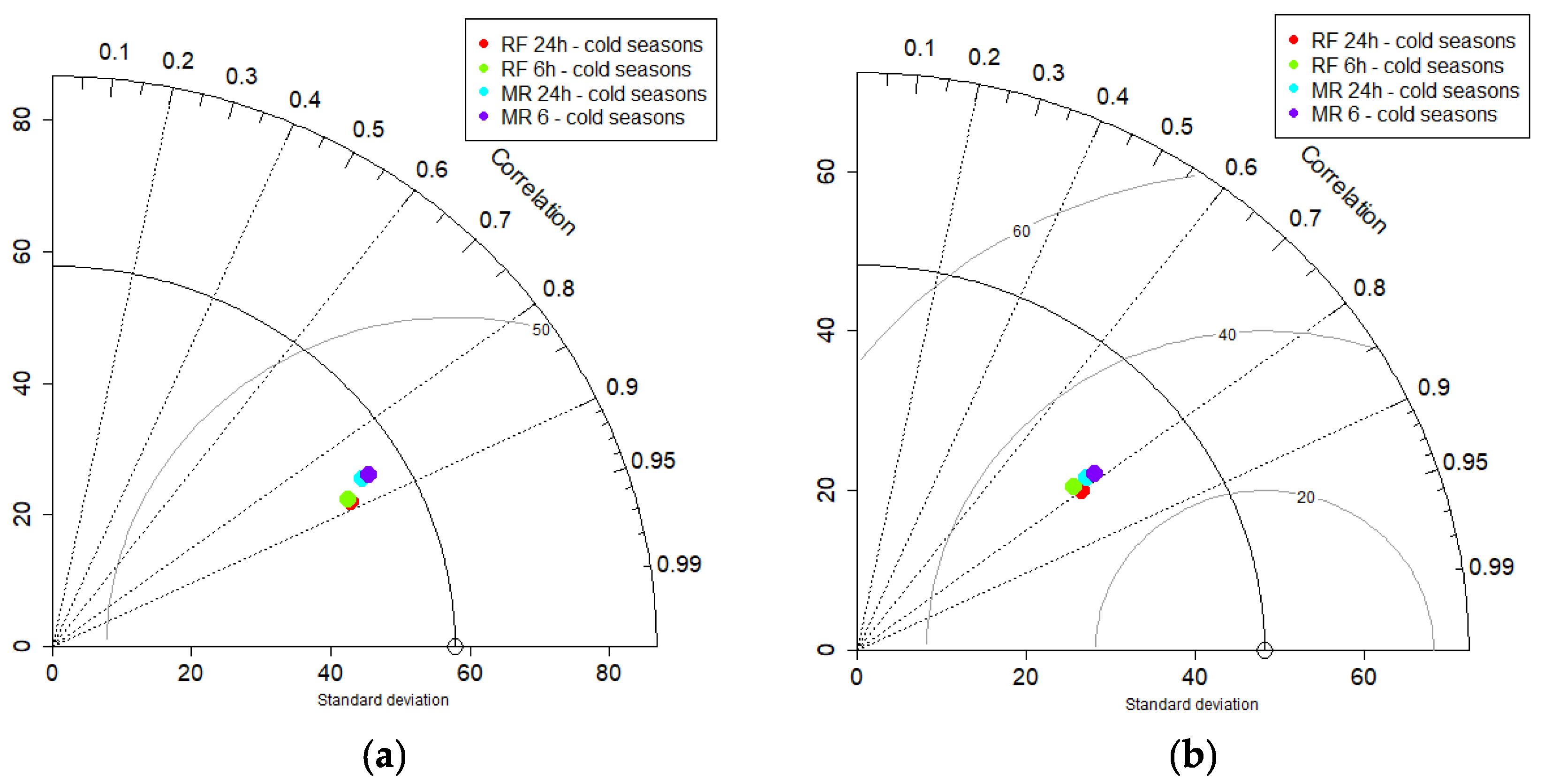
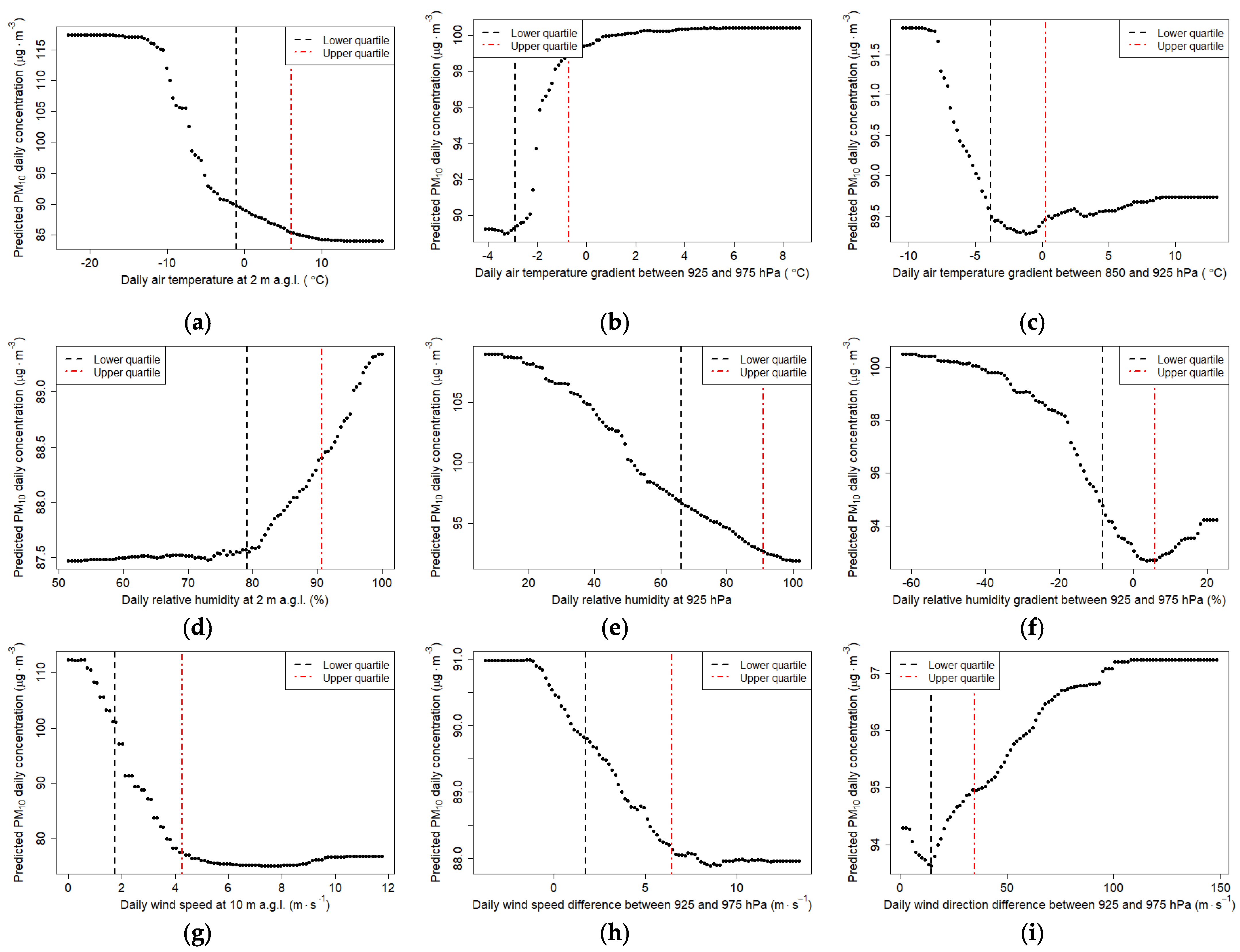
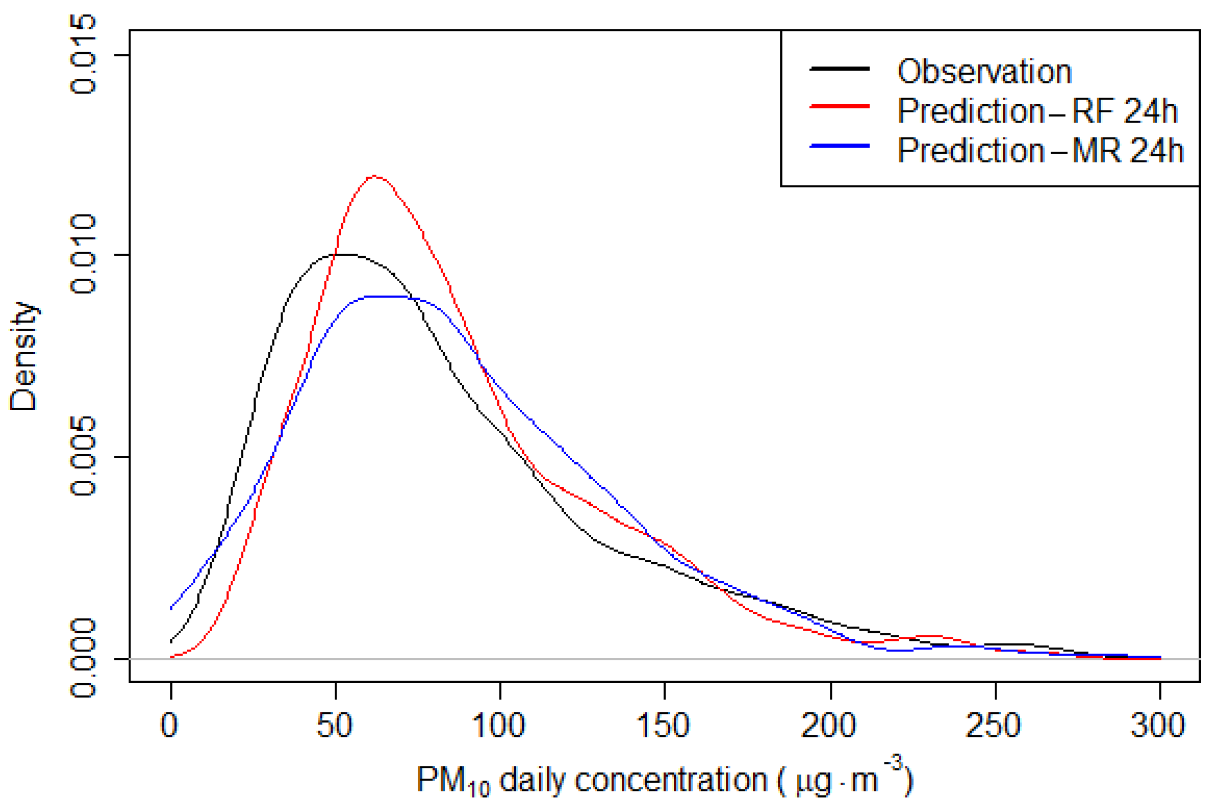
Random Forests Analyses

At the first step the Random Forests and multilinear regression models were built to predict daily PM10 concentration with the use of two different meteorological data resolution sets (6-h resolution and daily averages from 6-h resolution data). The Boruta variable selection method was applied for Random Forests models, and it showed that for the model which uses daily averages, the following parameters: daily cloudiness, wind direction changes in the layer between 925 hPa and 850 hPa and wind direction at 850 hPa were unnecessary. For the Random Forests model which uses meteorological parameters with 6-h resolution 28 of 111 selected variables were rejected by the Boruta method, including both circulation types, wind direction at 850 hPa, wind direction and wind speed change in layer between 925 and 850 hPa, relative air humidity at 2 m a.g.l. at 0, 12 and 18 UTC, wind direction at 925 hPa at 0, 6 and 18 UTC and day of week. The results of both Random Forests models were similar, the average value of mean absolute error (MAE) and root-mean square error (RMSE) for both models were equal 19.6 μg⋅m−3 and 26.9 μg⋅m−3, respectively. The Random Forests models analysis for specific measured PM10 concentration ranges 0–50 (25% testing data), 50–100 (40% testing data) and 100–200 (27% testing data) indicated that the RMSE error was equal respectively to 18, 20, and 32 μg⋅m−3. The group of observations with PM10 concentration exceeding 200 μg⋅m−3 was relatively small (5% testing data), and the RMSE for this group was the largest equal to 42 μg⋅m−3. An example plot presenting comparison observations with the Random Forests model forecast is included in Appendix C, Figure A6a). In Figure 3 the most important parameters affecting daily PM10 concentration are presented. Air quality on the previous day (PM10 daily concentration) was the most important parameter for both models. For the sake of clarity of Figure 3, this parameter was not presented in the chart owing to the large differences between the GINI Index for this parameter and the next one. The analysis of variable importance for both Random Forests models confirmed the similarity of the results. Apart from the parameters whose significant influence on air quality is well established (air temperature and wind speed at the ground and air temperature gradient), the key factor was also the gradient of relative air humidity and wind shear in the lowest troposphere (layer between 975 and 925 hPa; Figure 3a).
With the aim of analyzing the significance of individual parameters concerning the model accuracy, tests by removing a single variable from the model were performed (Figure 4). These studies also confirmed that the most important parameter was the PM10 concentration level on the previous day. The lack of this variable in the model affected on MAE increased by almost 25% compared to the forecast results where all parameters were included.
Studies of multilinear regression for both data groups were done for the same teaching and testing sets. Variable criterion with use of Akaike algorithm showed that for data with daily averages of meteorological parameters, six variables were excluded in the analysis: relative air humidity at 2 m a.g.l., wind speed at three pressure levels (975 hPa, 925 hPa and 850 hPa), relative humidity gradient in layer between 925 and 850 hPa and relative humidity at 850 hPa. The results obtained for multilinear models were slightly worse for the Random Forests model which used the same data set, RMSE and MAE for multilinear models were equal to 29 μg⋅m−3 and 21.4 μg⋅m−3, respectively. A comparison of results obtained from four Random Forests and multilinear regression models is presented in the Taylor diagram in Figure 5. The analysis of results presented at Figure 5 indicates that there are slight differences between the two model groups in Pearson correlation coefficient and standard deviation of predicted values. In the case of multilinear regression and meteorological parameters with 6-h resolution, the results of the multilinear model were close to the previous multilinear model. The application of the Akaike method to select the best parameters for the multilinear model caused a reduction of the parameters from 111 to 44 variables. The selection of crucial variables did not improve model performance, RMSE and MAE were equal to 29 μg⋅m−3 and 21.4 μg⋅m−3, respectively. In this case the application of the Random Forests model for numerous variables showed better results than multilinear regression. The comparison of observations with the multilinear model forecast with the use of daily averages of meteorological parameters presented at Figure A6b) in Appendix C indicates that the model underestimates PM10 daily concentration for values below 25 μg⋅m−3. In contrast, Random Forests models more often overestimate PM10 concentration than multilinear regression in the range between 0 and 50 μg⋅m−3 (Figure A7 in Appendix C).
In the second part, Random Forests and multilinear regression models were used to predict day-to-day changes of PM10 daily concentration. The same database as presented above was used in these studies, including measurements from the Balice station, ERA-5 reanalysis, two circulation types, day of the week, month, day of the year and PM10 daily concentration at the previous day. The analysis of Random Forests and multilinear regression models showed similar results, the values of RMSE and MAE were equal on average to 30 μg⋅m−3 and 20 μg⋅m−3, respectively. For this case hyperparameter tuning and parameter selection for Random Forests models did not significantly improve model accuracy (change of RMSE and MAE did not exceed 3%). It is worth to mentioning that variable selection with the use of the Boruta method for the Random Forests model which uses data with 6-h resolution were reduced from 110 to 27 variables. An example plot presenting comparison observations of day-to-day changes with the Random Forests model forecast is included in Appendix C, Figure A8b). In the case of a multilinear linear regression model with the same data set, stepwise the Akaike method selected 46 variables from 110 available. Verification of four models presented with the use of a Taylor diagram in Figure 6b indicates that the differences between them are negligible; however, comparison of density curves for Random Forests and multilinear regression with observations indicates that also the Random Forests model often predicts day-to-day PM10 concentration changes in a range between −10 and 25 μg⋅m−3 (Figure A9 in Appendix C). For both models groups the most important parameter was the PM10 concentration level on the previous day. Figure 6 presents parameters importance for Random Forests models affecting day-to-day PM10 concentration changes.
Analyses of the importance of variables presented at Figure 6 showed that the most important parameters were air temperature and wind speed near the ground and at the closest pressure level 975 hPa. It is worth mentioning that relative air humidity and relative air humidity gradient were more crucial parameters than air temperature gradient in the layer between 975 and 925 hPa concerning the prediction of day-to-day PM10 changes (Figure 6a). Two additional sensitivity tests were performed. Firstly, one for the whole period, without dividing the data set into two half-years and another one with training the model with data from 2000 to 2015 and testing it with data from 2016 to 2020 (also without dividing data set into cold and warm half-years). In both cases we achieved a similar order of importance of parameters for both Random Forests models as in Figure 4, while scores were slightly improved, e.g., with a decrease of RMSE around by 7 μg⋅m−3 for both models. It can be explained by adding a warm half-year to the data set that is characterized by lower values of PM10 concentration level. Results obtained by multilinear linear regression models were slightly worse for both tests, mean differences between Random Forests models were equal to 3 μg⋅m−3 for RMSE. As mentioned before, the main motivation for using Random Forests was to determine which meteorological parameters should be considered for further analysis, but a comparison of the accuracy of our forecasts with similar models (both physical and based on machine learning) shows also the good predictive potential of such an approach [60,61,62].
The optimized Random Forests model built to predict daily PM10 concentration based on the daily averages presented above was used to analyze the partial relationship between individual meteorological parameters and the level of the PM10 daily concentration. Figure 7 presents the partial dependence of predicted PM10 daily concentration for selected meteorological parameters. The plots show the value of the lower and upper quartiles in the analyzed cold half-years (dashed vertical lines). Detailed analysis of the daily thermal gradient between 925 and 975 hPa, has shown that predicted PM10 concentration did not differ significantly for the positive values of vertical gradients (the number of such days in all analyzed cold half-years did not exceed 25%—Figure 7b). For the range of the daily gradient values between −3 °C and 0 °C in the layer between 925 and 975 hPa, the influence of this parameter on the daily value of the PM10 concentration increases significantly. During the days without absence of the elevated inversion in the layer between 850 and 925 hPa, the predicted value of PM10 concentration was close to the minimum value (low statistical importance). When the daily temperature gradient in the layer between 850 and 925 hPa decreases below −3 °C, a significant increase in the predicted pollutant concentration can be observed. The plots of the dependence of the air humidity at the ground (Figure 7d) and at the pressure level of 925 hPa (Figure 7e) on predicted PM10 concentration has shown a different relationship. For the days when daily relative humidity of 2 m a.g.l. exceeds 80%, there is a linear increase of the predicted daily PM10 concentration. On the other hand, with a decrease in relative humidity at the height of 925 hPa the predicted PM10 concentration increases. The plots of predicted PM10 concentration from the relative humidity gradient in the layer between 925 and 975 hPa have shown gradual deterioration of air quality with the decrease of humidity gradient in the range of from 0 to −25%. The relationship between the average daily wind speed at 10 m a.g.l and predicted air pollution level presented at Figure 7g indicates a strong decrease of PM10 concentration for the wind speed in the range from 0 up to 5 m⋅s−1; above this value the increase of wind speed did not significantly improve the air quality in the city. The relationship between the vertical wind shear in the layer between 925 and 975 hPa and the pollution concentration is presented in Figure 7h,i. When wind shear increases wind speed in the vertical profile, the crucial point is the exceedance of 5 m⋅s−1. For such situations the increase in the speed difference between layer 925 and 975 hPa does not significantly improve the air quality. When the wind shear is associated with a significant change in the wind direction between the level of 925 and 975 hPa, an increase in the difference in wind directions negatively affects the predicted air quality in the valley.

4. Discussion

The statistical analysis of the impact if meteorological conditions and atmospheric circulation types on air quality in Kraków with the use of machine learning methods made possible an objective selection of crucial parameters influencing the pollutant concentration level. In the studies presented, we have compared results from multilinear regression and the Random Forests method to predict daily PM10 concentration and its day-to-day changes for two sets of input data which differed in the temporal resolution of meteorological parameters. The application of 6-h resolution meteorological data in comparison with daily averages to predict daily PM10 concentration and its day-to-day changes showed similar results for both methods. This confirms the statement that the use of daily averages of meteorological parameters is sufficient to predict PM10 daily concentration a day ahead. Studies of the importance of variables’ in predicting PM10 day-to-day changes the with the use of 6-h resolution data indicated that the number of crucial parameters was significantly lower than for predicting PM10 daily concentration for the Random Forests model (equal to 27 from 111 possible variables). It is also worth mentioning that in the case of predicting PM10 concentration with the use of numerous variables (6-h data resolution), the multilinear regression model significantly reduced the number of variables while the Random Forests model selected more variables as important. Analyses of model performance showed that for this case Random Forests results were better than for multilinear regression models.
Additional tests with the use of measurements from October 2000 to September 2020 were carried out to estimate the impact of changes in meteorology and emissions during the recent cold season (October 2021 to December 2021). Eight different sets of training data were prepared for tests for Random Forests models and multilinear regression models (sets of two temporal resolutions: 6-h and daily averages; data for cold half-years only and for both half-years; training data for period from October 2000 to September 2020 and from January 2015 to September 2020). Analysis of the shorter period for model training was done to answer the question how models’ performance is affected. An analysis of Taylor diagram plots (Figure A10 in Appendix C) indicated that the multilinear regression models had a higher standard deviation than the observations, indicating an excessively high variability of predicted PM10 concentration. The results obtained from Random Forests models were closer to the observations than the results from linear regression models (lower value of RMSE and standard deviation closer to the observation’s). Secondly, using shorter periods for model training showed better results (lower RMSE and lower overestimation of PM10 concentration), however in individual smog episodes PM10 daily concentration was underestimated in comparison with forecasts using a longer training data set (Figure A11 in Appendix C). Analysis of the time course of predicted PM10 concentration showed that the multilinear model in some cases overestimated the PM10 decrease, while the Random Forests model performed better.
The conducted experimental studies (based on data from 2021) have shown that such analyses should take into account the circular data with greater resolution than the daily one. Considering only one type of circulation for the whole day does not make it possible to take into account the dynamics of circulation changes, which is particularly high over Central Europe in winter. On the basis of the existing classifications, especially the local one, a method of assessing the atmospheric circulation should be developed, taking into account the daily course (at least with 3 h resolution).
Furthermore, more detailed analysis of the importance of individual parameters on PM10 daily concentration level was available with the use of the Random Forests model. The results obtained were used in further analysis to investigate the dispersion of selected parameters for individual types of circulation.
The study on the influence of atmospheric circulation patterns on air quality made it possible to distinguish the dominant circulation types during which the probability of occurrence of poor air quality (Group 1) and a significant improvement in air quality conditions (Group 2) was the highest. Days with the high PM10 concentration at cold half-year, occurred mostly during the advection of air masses from the S-SW sector, non-directional anticyclonic situations (Ca + Ka type) and also anticyclonic situations with air advection from the W-NW sector. Such days were characterized by lower wind speed and air temperature at ground level and greater stability of the atmosphere during the day and night periods in comparison with days not assigned to both special groups (remaining days). According to the Mann–Whitney U test, the distribution of daily sums of precipitation was similar for dominant circulation types for days in Group 1 and remaining days, but the frequency of precipitation was lower for days in Group 1. Furthermore, during the daytime for days with high PM10 concentration, a local minimum of relative air humidity at level 925 hPa occurred frequently. The partial dependence of meteorological parameters obtained from the Random Forests model has also confirmed the negative effect of strong negative relative humidity gradient in layers between 925 and 975 hPa on air quality. In this case, advection of dry air masses at a height of 925 hPa, especially frequent for the S + SWa and W + NWa types, contributed to the increase in the stability of the atmosphere in the valley and resulted in a longer persistence of humid cold air pool. During the winter, when foehn wind occurs, there is often the advection of warm and dry air masses above the analyzed region [63]. Additionally, previous studies pointed out that circulation types S + SWa, Ca + Ka enhance the occurrence of fog in Kraków which confirms the poor air pollution dispersion conditions linked to those circulation types [64]; the occurrence of haze and fog episodes is studied widely in different parts of the world in the context of air pollution control [65].
The second case studied consisted of days characterized by a significant improvement of air quality (Group 2). A significant reduction in the PM10 daily concentration occurred mostly for three circulation patterns (air advection from W-NW sector and cyclonic type with differentiated air advection—Cc + Bc type). These days were characterized by increased wind speed and a greater share of days with precipitation in comparison with remaining days. Atmospheric stratification (relative air humidity and air temperature gradient) was similar for dominant circulation patterns for days assigned to Group 2 and to remaining days. Near-ground temperature inversion for days in Group 2 during daytime almost did not occur, which was confirmed by local measurements and ERA5 reanalysis. It is also worth mentioning that during these days, the local maximum of relative air humidity in the layer 925 hPa during daytime occurred frequently.
Days with anticyclonic conditions with air advection from the W-NW sector are characterized by changeable weather conditions, which contributed to improvement or deterioration of air quality conditions during the cold half-year. The improvement is observed when air masses could penetrate into the valley and remove the cold air pool, while deterioration can be seen when air masses pass over the valley. Studies conducted over the region of the Dead Sea Valley using a high resolution WRF model [66] indicated that foehn wind intrusion into the valley depends on synoptic and mesoscale conditions which affect the vertical structure of the lower troposphere. For the cases with a high stable layer over the Dead Sea Valley, the foehn reached the valley floor, while during a low stable layer, it did not.
Studies of air quality in cold and warm half-years have shown that weak wind speed is one of the most important factors which deteriorates air quality. Owing to this fact circulation patterns which are characterized by weak wind speed, caused by the interaction of local orography (air advection from S-SW and W-NW sectors) and also atmospheric stagnation were the most important (non-advective types with anticyclonic situation, according to Niedźwiedź: type Ca + Ka). The high importance of wind speed on air quality was confirmed by numerous previous studies [3,67,68]; however, studies of the partial dependence of meteorological individual parameters for daily PM10 level showed nonlinear dependency [31].
Furthermore, studies of individual meteorological parameters have shown that vertical wind shear can worsen but also improve air quality in the valley. An increase of wind speed difference between the layers 925 and 975 hPa had a positive impact on air quality. On the other hand, strong wind shear associated with a change of the wind direction in vertical profile affects the deterioration of air quality by reducing the height of the mixing layer during the daytime. The study of the PM10 concentration vertical profiles in Kraków presented in the work of Sekula et al. 2021 [69] indicate that this phenomenon often occurs at the valley bottom height (approx. 100 m a.g.l.). During the cold half-year, poor dispersive conditions are more frequent than in the warm half-year, which in combination with high rates of emission from the residential sector led to accumulation of pollutants inside PBL. Analysis of the deseasonalized multiyear PM10 trend has shown that in the decade 2011–2020 a negative trend was observed which may be linked to the positive trend of air temperature.
According to the Random Forests model, adding a vertical gradient between neighboring pressure fields improved the quality of the PM10 level forecast. Other studies concerning application of machine learning methods in air quality forecasting confirmed that meteorological parameters like, wind speed, air temperature, relative air humidity and atmospheric precipitation were important factors affecting air quality [70]; however, studies of the effect of atmospheric precipitation on the concentration of particulate matter showed that it mainly washes out coarse particles while having little effect on fine particles [71]. Attention should also be paid to the representation of the atmospheric stability in the machine learning models; in this research we can distinguish two approaches: the application of planetary boundary layer height [31,72] or a more complex one with the application of meteorological conditions at different atmospheric pressure levels [73]. Owing to the fact that the estimation of planetary boundary layer height in numerical atmospheric models still requires validation and further development [74,75] we would like to suggest applying vertical profiles of atmosphere rather than PBL height in studies.

5. Conclusions

The analysis of air quality conditions in the multiyear period has proved that wind speed, air temperature, atmospheric stability connected to relative humidity gradient and air temperature gradient at lower troposphere and the occurrence of precipitation significantly influences pollutant concentrations. Apart from the non-directional anticyclonic conditions which affect air stagnation, air advection from the S-SW sector, strongly modified by local topography, has usually caused an increase of PM10 levels in the study area. Studies have shown that for the region analyzed the direction of air advection and its intensity is of greater importance than the type of pressure system concerning the impact on PM10 levels. Certain types of circulation can be indicated as significant both in terms of improving the dispersion of pollution and its deterioration; this is the result of the modification of large-scale processes by orography and near-ground atmospheric conditions. For example, air masses advection from the W-NW sector may strengthen near-ground thermal inversion and reduce wind speed in the valley, but it can also break thermal inversion in the valley and topographically channel the air flow. Research has indicated that particular types of circulation may affect the deterioration of air quality conditions in the cold half-year. During these circulation types lasting for a few or several days, a continuous increase of air pollution can be observed. Sometimes it leads to extremely high values of PM10 concentrations (e.g., types S-SW, W + NWa).
The analysis of the number of days with PM10 levels exceeding the daily limit in the study period showed that the emission reduction contributed to a significant improvement in the air quality in the city; however, the occurrence of days with poor air quality in the future is very likely due to the strong influence of meteorological conditions on that element. The number of days with low thermal inversion in the 975–925 hPa layer in a cold half-year turned out to be particularly important. Significant factors influencing the improvement of air quality in the cold half-year were the occurrence of longer rainfall (rainfall during the day and night), high daily wind speed in the valley and negative air temperature gradient.
One of the limitations in the studies presented above is the assignment of a single circulation type to the whole day; on days when an atmospheric front or the pressure center passes over a certain area, the meteorological conditions may change significantly during the day. Therefore, for the detailed analysis of atmospheric circulation, the daily fluctuations of circulation conditions should be taken into account. Currently, studies on application of the Convolutional Neural Network in automatic classification of atmospheric circulation according to the Niedźwiedź classification with the use of ERA5 reanalysis are conducted in our research group. The first results obtained are promising, however some model optimizations are still necessary.
Analysis of hourly PM10 concentration data and meteorological parameters with the use of cross correlation function have shown the occurrence of delayed time response of PM10 concentration level in the city to the change in meteorological conditions. For instance, at Krasińskiego station, the delayed time response obtained for the PM10 level for the wind speed, wind gusts, air temperature, as well as the ground thermal gradient was equal to 2 h; however, it should be mentioned here that air quality in the city may vary significantly on spatial and temporal scale as it was presented in other studies [8]. Further research on the intra-city spatial dependency from meteorological parameters and circulation patterns is necessary from the point of view of habitability and health risk.
Previous studies indicated that each technique of circulation patterns classification has some limitations e.g., there is a problem of equally sized classes, separation of different types, seasonal or inter-annual variability of a class frequency. In the case of the subjective classifications, there are high inter-annual variability and larger long-term trends of the frequencies of the types’ in comparison to the automated circulation classification methods; however, subjective classification includes important expert knowledge concerning analyzed geographical regions, which is difficult to formulate in precise rules for automated classification methods [52]. In conclusion the authors would suggest using local circulation classification methods in studies for different regions, owing to the effect of topography on modifications of atmosphere dynamics; however, because of the obvious limitations of the use of manual approaches, connected to their subjective nature, it seems that the best solution would be to use a local subjective classification of circulation types, which could be automated. Such approaches are known in the literature, although, they were applied in larger spatial scales [51].
Owing to the fact that machine learning methods create great opportunities in air quality studies, further development works are planned using the Random Forests method to analyze and forecast air quality on a larger spatial scale (e.g., cities in Central Europe) by supplementing the model with additional data such as land cover, topography, and turbulence parameters, as well as the results from operational forecasts of numerical air quality models to improve model accuracy. The further step in air quality studies will be an application of multi-step time series forecasting to model daily cycle of air pollution but also to predict daily pollution levels for three days ahead by using weather forecast and air pollution levels on the current day [75,76]. The next direction of development of the current research focuses on the analysis of spatial and temporal variability of pollution for large cities using data from air quality stations as well as non-governmental air quality systems. The first tests of using convolutional neural networks to determine air pollution level with respect to circulation patterns over larger domains are very promising, and so it is also planned to further investigate those methods.

Author Contributions

Conceptualization, P.S., Z.U., A.B. and M.Z.; methodology, P.S., Z.U. and A.B.; software, P.S. and B.B.; validation, P.S. and B.B.; formal analysis, P.S.; investigation, P.S., A.B., Z.U., B.B. and M.Z.; resources, P.S., Z.U., A.B. and B.B.; data curation, P.S. and B.B.; writing—original draft preparation, P.S.; writing—review and editing, P.S, B.B., Z.U., M.Z. and A.B.; visualization, P.S. and B.B.; supervision, P.S.; project administration, P.S.; funding acquisition, Z.U., M.Z. and B.B. All authors have read and agreed to the published version of the manuscript.

Funding

This research has been partly supported by the EU Project POWR.03.02.00-00-I004/16 (PS). This work was (partially) supported by the AGH UST statutory tasks No. 11.11.220.01/1 within subsidy of the Ministry of Science and Higher Education.

Institutional Review Board Statement

Not applicable.

Informed Consent Statement

Not applicable.

Data Availability Statement

Publicly available datasets were analyzed in this study. This data can be found here: Chief Inspectorate for Environmental Protection (CIEP). Available online: https://powietrze.gios.gov.pl/pjp/archives (accessed on 8 March 2022). Calendar of circulation types. Available online: http://www.kk.wnoz.us.edu.pl/nauka/kalendarz-typow-cyrkulacji/ (accessed on 8 March 2022). Institute of Meteorology and Water Management, National Research Institute. Available online: https://danepubliczne.imgw.pl/datastore (accessed on 8 March 2022).

Conflicts of Interest

The authors declare no conflict of interest. The funders had no role in the design of the study; in the collection, analyses, or interpretation of data; in the writing of the manuscript, or in the decision to publish the results.

Appendix A

Air quality data analysis with measurements from station at Krasińskiego St. has shown significant differences in the distribution of the daily PM10 concentration during warm and cold half-years. The multiannual trend of the number of days with exceedance of limit 50, 100, and 200 μg⋅m−3 were calculated for cold and warm half-year separately. The period covered from October 2000 to September 2020. For a selected number of days a linear curve was fitted by using the Theil-Sen estimator [77] provided in the RobustLinearReg R package was fitted [78]. The number of days with an exceedance of the daily pollution level (equal to 50 µg⋅m−3) is characterized by a decreasing trend equal to −5.33 days/year for the warm half-year (R-squared was equal to 0.51), while for the cold half-year the number of days with exceedance of 50 µg⋅m−3 has no positive or negative multiyear trend (Figure A1a,b). During the cold half-years in the period 2000–2020 there was a visible negative trend of the number of days with exceedance of limit 100 μg⋅m−3 equal to −2.31 days/year with R-squared equal to 0.23. In the study period, there are visible fluctuations in the number of days with exceedance of the daily PM10 limit, during warm and cold half-years (Figure A1c,d), which clearly indicates the impact of weather conditions on the frequency of smog episodes.
Figure A1. Distribution of daily PM10 concentration at the Krasińskiego station in the cold (a) and warm half-year (b), and the number of days with exceedance of limit 50, 100 and 200 µg⋅m−3 in the cold (c) and warm (d) half-year in the period 2000–2020.
Sustainability 14 03388 g0a1
In an effort to better analyze the multiannual trend in the period from October 2000 to September 2020 of the PM10 concentration, the Theil-Sen estimator with the switched option of seasonal trend decomposition using loess was used (Figure A2). By default, the values of the averaging period and autocorrelation were used, equal to month and the 95% confidence level. The function used for this calculation was provided by the openair R package [79]. Analysis has shown that during the analyzed period there is a negative trend equal to −1.94 μg⋅m−3/year. In the study period 2000–2020, the months of January 2001 and 2006 differ significantly from the entire study period. This situation was caused by anomalies of air temperature at 2 m a.g.l. (Figure A3) and atmospheric stability in the layer between 975 and 925 hPa (not shown in the article). Detailed analysis of the multiyear trend of PM10 has shown that stronger negative trend of PM10 concentration occurred during the period 2011–2019 than for 2002–2010, equal to −2.54 μg⋅m−3/year and −0.64 μg⋅m−3/year, respectively. For the same sub-periods, air temperature trends also differ significantly, in the period 2011–2019 the trend was equal to 0.21 °C/year, while for the earlier period amounted to −0.07 °C/year. On the other hand, analysis of the deseasonalized air temperature gradient in the layer between 975 and 925 hPa and daily wind speed at 10 m a.g.l. did not show any significant trends throughout the multiannual period (not shown in the article). The significant positive trend in air temperature in the last decade may be a crucial factor in determining PM10 emission in the cold half-years. Studies of warm temperature extremes for Central Europe in the period 1950–2020 have shown a positive trend of intensity and frequency of hot events during winter periods [80].
Figure A2. Deseasonalized multiyear trend of PM10 daily concentration in period from October 2000 to September 2020. *** indicates that the obtained trends are significant to the levels 0.001.
Sustainability 14 03388 g0a2
Figure A3. Deseasonalized multiyear trend of air temperature at 2 m a.g.l. in period from October 2000 to September 2020. ** indicates that the obtained trends are significant to the levels 0.01.
Sustainability 14 03388 g0a3

Appendix B

Appendix B.1. Niedźwiedź Circulation Classification

The classification of circulation types for Southern Poland [81] is available for the period from September 1873 to the present day. The classification was based on the typology of atmospheric circulation developed by Lamb [82] for the British Isles, with some modifications, especially regarding nonadvection situations. On the basis of synoptic maps of Europe, the direction of air mass movement (N, NE, E, SE, S, SW, W, NW) and the type of baric system (a—anticyclonic situation, c—cyclonic situation) were determined. Finally, 16 types of atmospheric circulation were distinguished. In addition, there are two non-advectional types: Ca—high-pressure center and Ka—anticyclonic wedge or ridge, and two cyclonic types of differentiated air advection: Cc—low pressure center and Bc—cyclonic troughs. The aric col and low-gradient situations, which are difficult to classify, are marked with the letter “x”. Thus, the entire classification includes 21 types (10 anticyclonic types, 10 cyclonic types and one indefinite type). By combining adjacent types, a shortened version is also obtained for 11 situations (N + NEa or c; E + SEa or c; S + SWa or c; W + NWa or c; Ca + Ka, Cc + Bc, x), which is useful in studies of periods shorter than 30 years [29].
Due to the fact that the study period covers 20 years, the classification version with 11 types of circulation was used, in order to increase the size of samples and obtain more reliable statistical results. For the analyzed period from October 2000 to September 2020 the multiannual trend was determined for warm and cold half-years, respectively, for each of 11 Niedźwiedź circulation types (Table A1 in Appendix B). During each half-year, the number of days with a specific circulation type were determined. At the next step, linear curves were fitted for each circulation type by using the Theil-Sen estimator from RobustLinearReg R package. Analysis has shown that the strongest negative trend was observed for type Ca + Ka during the warm and cold half-year, and it was equal to −0.73 and −0.60 days/half-year, respectively. Studies of 21 Niedźwiedź circulation types has shown that a strong negative trend was observed for type Ca + Ka was caused by decrease of number of days with anticyclonic wedge or ridge situation (type Ka), for which the trend was equal −0.76 and −0.57 days/half-year, for cold and half-years, respectively (not shown in the article). During the cold half-year multiyear trend of circulation types S + SWa and N + NEc was equal to 0.27 and 0.21 days/half-year, while for circulation type S + SWc the multiyear trend was negative (equal to −0.2 days/half-year). For the warm half-year, the trend of cyclonic conditions with air masses advection from sectors N–NE, S–SW was positive equal to 0.44 and 0.26 days/half-year, respectively. On the other hand, multiyear trend of W + NWc and Cc + Bc types in warm half-years were negative and equal to −0.50 and −0.33 days/half-year, respectively. The total frequency of particular atmospheric circulation types in the period October 2000–September 2020 in warm and cold half-years is presented in Figure A4 in Appendix B.
During the warm half-year, the shares of nonadvection anticyclonic types (Ca + Ka) and cyclonic types with differentiated air advection (Cc + Bc) are the highest and equal to 15% and 16%, respectively. Air advection from the W–NW sector during cyclonic and anticyclonic situations occurs often, and comprises 23% of all cases.
The cold half-year period differs significantly from the warm one; the share of air advection from the SW-NW sector (cyclonic and anticyclonic types) is greater by 15% in cold half-year than in the warm one. Parallel, the share of cyclonic types with differentiated air advection during the cold half-year is lower by 6% compared to the warm half-year.
Table A1. Multiyear trend of 11 atmospheric circulations according to Niedźwiedź classification in warm and cold half-years in period from October 2000 to September 2020.
Circulation TypeCold Half-YearWarm Half-Year
Trend (Day/Half-Year)R-SquaredTrend (Day/Half-Year)R-Squared
N + NEa−0.090.010.190.06
E + SEa0.100.010.130.02
S + SWa0.270.070.130.04
W + NWa0.000.000.170.02
Ca + Ka−0.600.23−0.730.35
N + NEc0.210.020.440.12
E + SEc0.150.020.000.00
S + SWc−0.200.020.260.12
W + NWc0.000.00−0.500.16
Cc + Bc0.160.04−0.330.17
x0.120.060.000.00
Figure A4. Frequency of Niedźwiedź circulation types during the period October 2000—September 2020 in warm and cold half-year.
Sustainability 14 03388 g0a4

Appendix B.2. Lityński Circulation Classification

One of the classifications of atmospheric circulation types widely applied in Poland is the threshold-based method proposed by J. Lityński. Lityński developed his objective classification to be applied to Poland and Central Europe [38,53]. Synoptic types were defined using the following indicators: zonal (Ws), latitudinal (Wp) and Warsaw air pressure (Cp) using sea-level synoptic maps over an area defined as 40–65 °N and 0–53 °E. The Ws indicator was derived using a formula for an average longitudinal component of the geostrophic wind. A conversion of this formula was used to determine the latitudinal circulation indicator [38]. The direction of air advection and the type and strength of the pressure systems were determined on a frequency distribution of the Ws, Wp and Cp indicator values and using a three-class equal-probability system. The thresholds employed to calculate the Wp, Ws and Cp indices change from month to month, which results in flattening the seasonal cycle of the occurrence of circulation types [38]. The resulting air advection type was described by three numeric parameters: Wp, Ws and Cp. The following symbols were used to denote the Ws indicator: E (eastern) for most negative values, 0 for near-zero values and W (western) for most positive values. Similarly, the Wp indicator was denoted by the symbols: N (northern) for most negative values, 0 for near-zero values and S (southern) for most positive values. Cp air pressure classes were marked: C (cyclonic), 0—near-zero and A (anticyclonic). These circulation type symbols were combined with the Wp and Ws indicators class symbols, and finally, one of the three Cp air pressure class symbols were added. Lityński distinguished 27 circulation types, three non-advective types (symbol Oo, Oc, Oa) and 8 directional types (with 3 types, cyclonic, anticyclonic and intermediate type, known as the near-zero type). It is worth to note that Litynski’s classification system, as one of the scalable methods, is part of the COST 733 classifications catalogue [83]. In the current artile, the Lityński classification has been used with modifications introduced by Krystyna Pianko-Kluczyńska [63]. Recent studies confirm the high level of comparability in the course of circulation indices according to the classifications of Niedźwiedź and Lityński [29].
Figure A5 in Appendix B presents the frequency of Lityński circulation types during the warm and cold half-year of the study period. For the analyzed period from October 2000 to September 2020, the multiannual trend was determined for warm and cold half-years, respectively, for 27 Lityński atmospheric circulation types. During each half-year, the numbers of days with a specific type of circulation were determined. In the next step, for each circulation type, linear curves were fitted by using the Theil-Sen estimator from the RobustLinearReg R package. Detailed analysis has pointed out that during the warm half-year share of circulation types Ec and Wa have the strongest negative trend equal to −0.25 and −0.21 days/half-year, respectively. F°or the type Oa in the warm half-year, the strongest positive trend equal to 0.25 days/half-year was observed. During the cold half-year share of types NEa and Sc are characterized by the strongest negative trend equal to −0.22 and −0.25 days/half-year, respectively. On the other hand, for SEo, SWc, Wa and NWa positive trend equal on average 0.28 days/half-year was observed. Detailed information on individual circulation types during the cold and warm half-year in the period from October 2000 to September 2020 was included in Appendix B, Table A2. In comparison with warm half-year, during cold half-year there is a visible decrease of air advection from the NE direction, with a significant increase of air advection from the SW direction. It is worth noting that the share of cyclonic types with air advection from the W–NW sector is greater during the cold season, whereas anticyclonic types with air advection from the same direction have a lower frequency in comparison with warm half-year.
Figure A5. Frequency of Lityński circulation types during the period October 2000—September 2020 in warm and cold half-year.
Sustainability 14 03388 g0a5
Table A2. Multiyear trend of 27 atmospheric circulations according to Lityński classification in warm and cold half-years in period from October 2000 to September 2020.
Circulation TypeCold Half-YearWarm Half-Year
Trend (Day/Half-Year)R-SquaredTrend (Day/Half-Year)R-Squared
Nc−0.130.150.000.00
No−0.070.030.200.27
Na−0.040.00−0.090.00
NEc−0.030.000.000.00
NEo−0.110.070.080.04
NEa−0.220.120.000.00
Ec0.000.00−0.250.18
Eo0.000.000.130.03
Ea0.000.00−0.130.07
SEc0.110.040.000.00
SEo0.250.130.000.00
SEa0.000.000.000.00
Sc−0.250.06−0.110.02
So0.000.00−0.080.04
Sa0.000.000.000.00
SWc0.260.08−0.180.10
SWo0.000.00−0.110.13
SWa0.000.000.080.00
Wc0.000.000.130.07
Wo0.000.00−0.100.05
Wa0.270.13−0.210.14
NWc0.000.00−0.130.03
NWo0.140.080.000.02
NWa0.370.170.180.13
Oc−0.120.04−0.080.00
Oo0.000.000.110.03
Oa−0.190.110.250.13

Appendix C

Table A3. Height of PM10 daily concentration upper quartile in warm and cold half-years.
YearCold Half-Year (μg⋅m−3)Warm Half-Year (μg⋅m−3)
20014741
200210694
200313760
200411660
200516273
200614571
200713477
200815569
200912367
201013557
201113753
201213149
201313047
201410343
201511554
20169950
20179938
20188750
20198242
20207132
Figure A6. Scatterplot of predicted versus observed PM10 daily concentration (a) for Random Forests model and (b) multilinear regression model with daily meteorological parameters for the cold half-years.
Sustainability 14 03388 g0a6
Figure A7. Density plot observed and predicted PM10 daily concentration for Random Forests (RF) and multilinear regression (MR) model with daily meteorological parameters for the cold half-years.
Sustainability 14 03388 g0a7
Figure A8. Scatterplot of predicted versus observed PM10 day-to-day concentration changes (a) for Random Forests model and (b) multilinear regression model with daily meteorological parameters for the cold half-years.
Sustainability 14 03388 g0a8
Figure A9. Density plot observed and predicted PM10 day-to-day concentration changes for Random Forests (RF) and multilinear regression (MR) models which use daily meteorological parameters for the cold half-years.
Sustainability 14 03388 g0a9
Figure A10. Taylor diagram plots of predicted PM10 daily concentration for the period between October 2021 and December 2021 for (a) multilinear regression models and (b) Random Forests models for different training data sets.
Sustainability 14 03388 g0a10
Figure A11. Time course of observed and predicted PM10 daily concentration for period between October 2021 and December 2021 for (a) multilinear regression models and (b) Random Forests models with use of daily averages of meteorological data for both half-years for two different training periods.
Sustainability 14 03388 g0a11

Appendix D

Weather Conditions in Relation to the Circulation Types

The following section describes the distribution of the selected meteorological parameters for 11 Niedźwiedź classification types during the cold half-years in the analyzed period. Studies of daily wind speed for the cold half-year have shown that the lowest wind speed occurs during the advection from sector S–SW which is caused by the local topography (surrounded by highlands from the South, North and West—see Figure 1b). The weak wind in the valley was also frequent at stagnant anticyclonic situations (type Ca + Ka). The conditional probability of the occurrence of a daily wind speed below 1 m⋅s−1 was the highest for the circulation types S + SWa and Ca + Ka, slightly above 30%. For the other types, except for the S + SWc and W + NWa types, the conditional probability did not exceed 5% (for the S + SWc and W + NWa types equal 14% and 10%, respectively). The highest average value of the daily speed was determined for the type of circulation W + NWc, equal to 5 m⋅s−1.
The analysis of the mean daily cloudiness for the individual circulation types pointed out that the greatest variability of this parameter occurred for the types S + SWa, Ca + Ka and E + SEa (interquartile ranges were greater than 4 oktas). On the other hand, the lowest variability of daily cloudiness was observed for cyclonic types with advection from sectors E–SE and W–NW, as well as for low-pressure center and cyclonic troughs (interquartile range for these types ranged from 0.7 to 1.6 oktas). The conditional probability of a day with daily cloudiness not exceeding 2 oktas was the highest for the circulation types S + SWa and Ca + Ka, equal to 28% and 26%, respectively. The results obtained are consistent with the research of a longer multiyear period [28].
The median of the daily sum of precipitation differs significantly for cyclonic and anticyclonic conditions; for anticyclonic types, the value did not exceed 1 mm/day. The highest value of the median daily precipitation was determined for the types Cc + Bc and E + SEc, equal to 2.5 mm/day. The percentage of days with daily precipitation above 0.1 mm/day was the lowest for anticyclonic types S + SWa and Ca + Ka, equal to 16% and 18%, respectively. For cyclonic types, except for the type S + SWc, the share of days with precipitation in the cold half-years was greater than 70%. A significantly lower share of days with precipitation for the S + SWc type equal to 53% is related to the orographic barrier of the Western Carpathians, which as a result affects the air temperature and the humidity of the air masses and spatial distribution of the atmospheric precipitation [76].
The distribution of the daily relative humidity at the ground level in the cold half-years is similar for most circulation types, except types N + NEc, E + SEc, Cc + Bc and x for which a higher daily humidity was observed. For the selected circulation types, the lower quartile of daily relative humidity ranged from 83% to 87%, while the average value of the lower quartile for the remaining types is equal to 78%.
Analysis of the daily air temperature showed that the largest interquartile range was measured for Ca + Ka and E + SEa types. It should also be noted that for the selected types the value of the lower quartile was the smallest, equal to −4.6 and −3.9 °C, for the types E + SEa and Ca + Ka, respectively. Low values of the daily air temperature for the Ca + Ka type are associated with strong radiative cooling of the surface with the cloudless sky. For days with anticyclonic condition with advection from sector E-SE, in most cases, the analyzed region is under the influence of a strong high-pressure center developed over the area of Eastern Europe and then moved into the West. For this circulation type, advection of polar continental air masses dominates (more than 75% of the cases). On the other hand, the highest values of the median daily air temperature occurred for the types Cc + Bc, W + NWc and S + SWc, equal to 3.9, 4.2 and 4.4 °C, respectively.
The analysis of the vertical profiles obtained from the ERA5 reanalysis indicated that the relative air humidity at pressure levels 925 and 850 hPa strongly depends on the direction of advection, during the day and nighttime periods. The air masses moving from the S-SW sector (for cyclonic and anticyclonic conditions) are characterized by much lower relative humidity than for the other types of circulation (the median value of relative humidity at 925 hPa at 12 UTC for both types were equal to 58 and 67%, respectively, while for the others it was within the range from 77% to 95%). Significant fluctuations in relative air humidity were also observed for stagnant anticyclonic situations (Ca + Ka) and anticyclonic conditions with advection from the W-NW sector at 0 UTC in the pressure level 850 hPa.
It should also be mentioned that for days with advection from the S–SW sector during the daytime and nighttime period, a strong decrease in relative humidity is visible in the layer 975–925 hPa. During the night, at 0 UTC, the median of relative humidity gradient between the levels 925 and 975 hPa for the selected types was lower than −13%, while for the remaining types, the humidity gradient varied between −5% and 4%.
During the day with advection from sector S–SW, a higher relative humidity gradient was observed compared to the remaining circulation types in the layer 925–850 hPa.
Analysis of air temperature at pressure levels 975, 925, and 850 hPa indicated that during the daytime air temperature at the height of 925 hPa is significantly higher for days with advection from the S-SW direction, than for the other types.
The median of the vertical temperature gradient in the layer 925–975 hPa during the night was the highest with the advection from the S–SW sector. During the day, the largest share of days with a positive vertical gradient was observed for the type S + SWa, equal to 30%. The statistically significant share of days with low thermal inversion was also observed for the types E + SEa and Ca + Ka, close to 16%.
Taking into account the distribution of all meteorological parameters for 11 Niedźwiedź classification types, the types Ca + Ka and S + SW (cyclonic and anticyclonic situation) are potentially the most important circulation patterns affecting the deterioration of air quality in the city. For the selected types, weaker wind speed at the ground level, higher frequency of thermal inversions, and stronger negative gradient of relative air humidity were observed in comparison with the remaining circulation patterns. The analysis also showed that the type E + SEa type can have a significant impact on air quality due to the occurrence of low daily air temperatures for this type of circulation.
Group 1: days with the highest PM10 concentration.
Table A4 presents the conditional probability of the occurrence of high PM10 mean daily concentration for individual types of atmospheric circulation during cold half-year, in the period 2000–2020, according to the Niedźwiedź classification.
Among the 11 types of circulation, only 5 types had the frequency greater than 10% in the cold half-year (S + SWa, W + NWa, Ca + Ka, S + SWc and W + NWc; Figure A4 in Appendix B). The worst air pollution conditions, that is, situations with the highest conditional probability of occurrence of high PM10 concentration in Kraków were almost the same: S + SWa (0.52), S + SWc and Ca + Ka (almost 0.4), and W + NWa (0.2), indicating that situations with air advection from the western sector, regardless of the baric center type, have less impact on the deterioration of air quality in the city than other types of circulation most frequent.
The highest number of days with PM10 concentration greater than the upper quartile in a cold half-year and exceeding daily limit value of PM10 occurred in December and January (162 and 195 days, respectively); the number of cases in November, February and March was similar: 140 days on average. The smallest number of such days was observed in October: 65 days.
Table A4. Conditional probability of the occurrence of high PM10 concentration during particular atmospheric circulation types during the cold half-year according to Niedźwiedź classification, number of days with selected circulation type and the number of days with high PM10 concentration for individual circulation types in the period 2000–2020.
Circulation TypeConditional ProbabilityNumber of Days with High PM10
Concentration
Total Number of Days in Cold Half-Year
N + NEa0.0612196
E + SEa0.1450354
S + SWa0.52202386
W + NWa0.20114562
Ca + Ka0.39171441
N + NEc0.1426190
E + SEc0.1221170
S + SWc0.37149403
W + NWc0.0422521
Cc + Bc0.1449348
x0.352674
Total number of days8423645
Figure A12 and Figure A13 present the weather conditions from the Balice synoptic station for each circulation type in division into three groups: days with high PM10 concentration (Group 1), days with a significant improvement of air quality (Group 2) and remaining days. Comparison of wind conditions for days assigned to Group 1 with the remaining days for four dominant circulation types (boxplots in blue frames in Figure A12a) has shown that these days are characterized by the weakest daily wind speed in the cold half-year. The Mann–Whitney U test calculated for days assigned to Group 1 and the remaining days for wind speed also confirmed that both groups differ statistically significantly for the four circulation types (p-value did not exceed 0.002; Table A5); however, it should be noted that wind speed distribution for circulation patterns S + SWa, S + SWc, and Ca + Ka did not differ significantly between the days from Group 1 and remaining days (the maximum difference of median and upper quartile was equal to 0.2 m⋅s−1 and 0.7 m⋅s−1, respectively). During the anticyclonic conditions with air advection from W–NW sector (type W + NWa) differences of wind speed distribution between days from Group 1 and remaining days were the highest from all four selected patterns (maximum difference of median and upper quartile was equal to 1.2 m⋅s−1 and 1.6 m⋅s−1, respectively). Studies of daily air temperature have shown that for days with high PM10 concentration for four selected patterns was lower than for the remaining days, the difference of median values ranged from 1.2 °C for type S + SWa to 3.3 °C for type Ca + Ka. It is also worth mentioning that the lowest daily air temperatures occurred for type Ca + Ka, which was partly related to small cloudiness during these days.
Figure A12. Boxplots of daily (a) wind speed and (b) air temperature for days with the highest PM10 concentration (Group 1), days with a significant decrease of PM10 (Group 2) and remaining days at cold half-year for 11 circulation types of Niedźwiedź classification for synoptic station Balice. The red and blue frames at subfigures a and b cover the dominant types of circulation in Group 1 and 2, respectively.
Sustainability 14 03388 g0a12
Detailed analysis of atmospheric precipitation showed that for anticyclonic conditions (types S + SWa, Ca + Ka, and W + NWa), the share of days with precipitation greater than 0.1 mm/day did not exceed 17% of all days in Group 1, and, moreover, precipitation occurred mostly at nighttime period (more than 90% of all cases). The median and upper quartile values of daily precipitation for these types of circulation were equal on average 0.6 mm and 1.6 mm, respectively. For the remaining days, the share of days with precipitation for types S + SWa and Ca + Ka were similar to days in Group 1 (differences below 10%), while for types W + NWa and S + SWc, the share of days with precipitation was higher compared to days from Group 1 by 25% and 14%, respectively. The Mann–Whitney U test has proven that the distribution of the sum of precipitation for all four types of circulation was similar for days assigned to Group 1 and for the remaining days.
Figure A13. Boxplots of daily atmospheric precipitation for days with the highest PM10 concentration, days with a significant decrease of PM10 and remaining days during cold half-year for 11 circulation types of Niedźwiedź classification for synoptic station Balice. The red and blue frames cover the dominant types of circulation in both groups of days.
Sustainability 14 03388 g0a13
Table A5. A p-value calculated with the Mann–Whitney U test between days assigned to Group 1 and remaining days in cold half-year calculated for daily wind speed, air temperature and atmospheric precipitation for four selected Niedźwiedź circulation types.
Circulation TypeWind SpeedAir Temp.Precipitation
S + SWa0.0000.0000.736
W + NWa0.0000.0000.813
Ca + Ka0.0020.0000.486
S + SWc0.0000.0000.748
The duration of near-ground thermal inversion for selected circulation patterns for days with the highest PM10 concentration, days with significant improvement of air quality and remaining days for day (from 6 to 17 UTC) and nighttime (from 18 to 5 UTC on the next day) were presented at Figure A14. For this purpose, air temperature measurements from the TV mast from two altitudes (2 and 100 m a.g.l.) were used. The lower limit of the occurrence of thermal inversion was set equal to +1 °C. The results presented in Figure A14 show that duration of thermal inversion at day is longer by 3–6 h for days in Group 1 compared to the remaining days for 3 of 4 selected circulation patterns (S + SWa, W + NWa, S + SWc). Furthermore, during days with air advection from sector S-SW (cyclonic and anticyclonic conditions), thermal inversion in special cases persisted for the whole daytime.
The duration of thermal inversion at night for days from Group 1 was the longest for days with circulation type S + SWa. For types S + SWc and W + NWa in most cases, the duration of thermal inversion was greater than 6 h.
Figure A14. Boxplots of air temperature near-ground inversion duration during daytime (a) and nighttime (b) according to the data from TV mast for selected Niedźwiedź circulation types for days with the highest PM10 concentration (Group 1), days with significant decrease of PM10 (Group 2) and remaining days during cold half-year in the period 2010–2020. The red and blue frames at subfigures a and b cover the dominant types of circulation in Group 1 and 2, respectively.
Sustainability 14 03388 g0a14
ERA5 reanalysis was used to analyze atmospheric stratification in the lower troposphere, in the first approach only thermal stratification was analyzed; however, the Random Forests machine learning methods presented in the previous subsection have pointed out that air humidity stratification and vertical wind profile were also crucial factors; therefore, the analysis has been extended. Boxplots of the air temperature and relative air humidity gradient for selected circulation types have been presented in Figure A15 and Figure A16. Analysis of the air temperature gradient in the layer 925–975 hPa has shown that atmospheric stability was stronger during night (00:00 UTC current day) and day (12:00 UTC) for all selected circulation types for days in Group 1 than for remaining days (Figure A15a,b, boxplots in blue frames). The differences in the median temperature gradient in the layer 975–925 hPa during the daytime ranged from 1 °C for type S + SWc to 2.5 °C for type S + SWa. On average, for more than 25% of days in Group 1, for four dominant circulation patterns, the temperature gradient in the layer 925–975 hPa was positive during the daytime. In the upper layer (850–925 hPa), the differences in thermal stratification between days assigned to Group 1 and the remaining days were not significant. The highest share of upper thermal inversion during the day for days assigned to Group 1 occurred for Ca + Ka type (56%); for the remaining types of circulation, the frequency of upper inversion was in the range from 39% to 43%.
Figure A15. Boxplot of air temperature gradient for selected circulation types for days with high PM10 concentration (Group 1), days with significant improvement of air quality (Group 2) and remaining days at cold half-year for layer 925–975 hPa at 00:00 UTC (a) and 12:00 UTC (b) and for layer 850–925 hPa at 00:00 UTC (c) and 12:00 UTC (d) from ERA5 reanalysis data for Kraków city.
Sustainability 14 03388 g0a15
Figure A16. Boxplot of relative air humidity gradient for selected circulation types for days with high PM10 concentration (Group 1), days with significant improvement of air quality (Group 2), and remaining days at cold half-year for layer 925–975 hPa at 00:00 UTC (a) and 12:00 UTC (b) and for layer 850–925 hPa at 00:00 UTC (c) and 12:00 UTC (d) current day from ERA5 reanalysis data for Kraków city.
Sustainability 14 03388 g0a16aSustainability 14 03388 g0a16b
Air humidity stratification during days assigned to Group 1 presented for four types of circulation during the nighttime is characterized by a stronger decrease of humidity in layer 925–975 than during the remaining days. Furthermore, during the day, for days with high PM10 concentration, local minimum of relative air humidity at the level of 925 hPa occurred frequently.
The number of cases in which relative air humidity in the 925–975 hPa layer was lower than in the neighboring layer (975- 850 hPa) by at least 10%, ranging from 18% for the S + SWc to 43% for S + SWa type. The percentage of such cases during the day and night for days with high levels of PM10 and days not assigned to both special groups is presented in Table A6.
Table A6. Frequency of days with a minimum of air relative humidity at 925–975 hPa during daytime and nighttime for days with high PM10 concentration and remaining days for selected Niedźwiedź circulation types.
Circulation TypeDays with the Highest PM10 Concentration (%)Remaining Days (%)
00:00 UTC12:00 UTC00:00 UTC12:00 UTC
S + SWa544819
W + NWa42524
Ca + Ka43345
S + SWc15181610
Analysis of relative air humidity at the level of 925 hPa for days assigned for Group 1 indicated that for the types S + SWa, W + NWa and Ca + Ka median values were significantly lower during the day and night in comparison with the days not assigned for both groups (the greatest difference in medians equal to 25% during day and night was observed for type W + NWa). Furthermore, for the days in Group 1 with circulation type W + NWa and Ca + Ka, the distribution of relative humidity was characterized by a significantly wider interquartile range than for the remaining days. The average daily value of the interquartile range for both selected types was equal 41% and 23% for days in Group 1 and remaining days, respectively. In the case of the circulation type S + SWc, the relative humidity distribution was similar for both groups of days (Group 1 and the remaining days). The relative humidity distribution at the level of 925 hPa for selected types of circulation was presented in Figure A17a). Analysis of the air temperature distribution at the level of 925 hPa for selected circulation types showed no significant differences for days assigned to Group 1 and the remaining days (Figure A17b). The study of the wind speed distribution at the level of 925 hPa for four types of circulation pointed out that the differences of this parameter between days in Group 1 and the remaining days are lower during the day than at night. The greatest differences of the wind speed distribution between days in Group 1 and remaining days at night were observed for W + NWa and S + SWc types. The median values of wind speed at night for days assigned to Group 1 were lower by 3.3 m⋅s−1 and 2.3 m⋅s−1 for W + NWa and S + SWc, respectively (not shown in the article). Furthermore, the analysis of the wind speed difference in layer between 925 and 975 hPa indicated that in the nighttime the wind shear was significantly weaker for the W + NWa and S + SWc types, while in the daytime period the distribution was similar or slightly higher than for the remaining days. For the Ca + Ka type, wind shear was the lowest among the four distinguished circulation types.
Figure A17. Boxplot of relative air humidity (a), air temperature (b), wind speed (c) at 925 hPa and wind speed differences between 925 and 975 hPa (d) at 12:00 UTC for selected circulation types for days with high PM10 concentration (Group 1), days with significant improvement of air quality (Group 2) and remaining days at cold half-year for layer 925–975 hPa from ERA5 reanalysis data for Kraków city.
Sustainability 14 03388 g0a17
Group 2: days with highest decrease of PM10 concentration.
The second Group of days selected in the cold half-year consists of days during which a significant decrease in daily PM10 concentration occurred in comparison with the previous day. Table A7 presents the conditional probability of the occurrence in a large decrease of PM10 concentration for individual types of atmospheric circulation, the number of days with a particular type of circulation and number of days with a significant decrease in PM10 concentration for individual types of circulation.
The significant improvement of the dispersion conditions occurred mostly with air advection from the W–NW sector at cyclonic and anticyclonic conditions and nonadvection cyclonic types (Cc + Bc). It is worth mentioning that during circulation type W + NWa the highest levels of PM10 concentration occurred, too. The highest conditional probability in significant decrease of PM10 concentration was obtained for cyclonic types Cc + Bc and W + NWc (0.29 and 0.25, respectively).
It should be mentioned that the number of days that meet the conditions of significant pollution decrease (more than 25% decrease and at least 20 μg⋅m−3) in individual months in the cold half-year is not even; the smallest number of cases meeting the criteria occurred in October (67 days), a similar number of days was selected for the months of November, February, and March (more than 100 days) and the highest number for the period from December to January (more than 120 days).
Table A7. Frequency of days with minimum of air relative humidity at 925–975 hPa during daytime and nighttime for days with high PM10 concentration and remaining days for selected Niedźwiedź circulation types.
Circulation TypeConditional ProbabilityNumber of Days with High PM10 ConcentrationTotal Number of Days in Cold Half-Year
N + NEa0.1835196
E + SEa0.1553354
S + SWa0.0625386
W + NWa0.1796562
Ca + Ka0.0628441
N + NEc0.3158190
E + SEc0.2543170
S + SWc0.1354403
W + NWc0.29150521
Cc + Bc0.2586348
x0.08674
Total number of days6343645
Analysis of weather conditions from the Balice synoptic station for selected circulation types (Figure A12 and Figure A13; boxplots in red frame) showed that air temperature did not differ significantly for days with a significant decrease of PM10 (Group 2) compared to days not assigned to both specific groups (remaining days). The p-value calculated with the Mann–Whitney U with significance level α = 0.05 test has also confirmed the similarity of both groups for these meteorological parameters (Table A8). The p-values obtained for wind speed and atmospheric precipitation were lower than 0.05, which pointed out that distribution in selected groups is statistically different. For the air temperature groups, the p-value were highest. The daily wind speed distribution for three selected circulation patterns were higher for days in Group 2 compared to the remaining days. The highest differences were observed for circulation type W + NWa (the median and upper quartile for this group were higher by 1.3 m⋅s−1 and 0.8 m⋅s−1), while for the remaining types (W + NWc and Cc + Bc), the wind speed was on average higher by 0.5 m⋅s−1.
The number of days with precipitation for days in Group 2 compared to days not assigned to both groups for dominant circulation patterns was higher by 18% on average. For the type W + NWa, the number of days with precipitation above 0.1 mm/day was equal to 53% of all days, and for the cyclonic types W + NWc and Cc + Bc it was equal to 84% and 88%, respectively. The sum of daily precipitation for the distinguished types was higher than for the remaining days, the smallest increase was observed for the anticyclonic type W + NWa (greater on average by 0.5 mm/day), while for the cyclonic types, the daily sum of precipitation was greater by more than 1 mm/day. The frequency of rainfall during the day and night was similar for all the distinguished types in Group 2.
Table A8. p-value calculated with the Mann–Whitney U test between days assigned to Group 2 and days not assigned to both groups in the cold half-year calculated for daily wind speed, air temperature and atmospheric precipitation for three selected circulation types from Niedźwiedź classification.
Circulation TypeWind SpeedAir Temp.Precipitation
W + NWa0.0000.7500.013
W + NWc0.0050.9180.000
Cc + Bc0.0000.8710.008
Analysis of intra-valley thermal stratification from TV mast data (up to 100 m a.g.l.) indicated that the length of the near-ground inversion persistence did not exceed 3 h for most of the cases. The duration of inversion in the night period was shorter for all the selected circulation types for days with a significant decrease in PM10 compared to the reference group that contained the remaining days (Figure A13; boxplots in red frames).
Analysis of the ERA5 data indicated that the vertical gradient of temperature and relative humidity did not differ significantly for the group of days with a significant improvement in air quality compared to days not assigned to both groups (Figure A15 and Figure A16 in Appendix D; data in red frames). Low thermal inversion in the 975–925 hPa layer during the nighttime period did not exceed 20% of all days for the selected types, and during the daytime, low thermal inversion almost did not occur. Upper thermal inversions in the layer 925–850 hPa during daytime accounted for more than 50% of cases, with the highest share equal to 60% for the W + NWa type. The vertical profile of relative humidity during the day was characterized by the local maximum at 925 hPa, the median relative humidity gradient in layers 975–925 hPa and 925–850 hPa was equal on average to +9% and −9%, respectively. The largest number of days, where relative humidity at the level of 925 hPa was higher than neighboring levels by at least 10%, occurred for the W + NWa type, equal to 33%, and the other types accounted for 17% of cases, on average. For the group of remaining days, similar humidity stratification, with local maximum relative humidity at 925 hPa, constituted from 20% for Cc + Bc to 28% for W + NWa type.
Analysis of relative humidity and air temperature at 925 hPa level during the daytime and nighttime period for the three distinguished circulation types did not show significant differences for the days assigned to Group 2 and the remaining days. The distribution wind speed at a pressure level of 925 hPa is for days in Group 2, for all selected types was higher during the day and night in comparison with the remaining days. The wind speed at night and day for all selected circulation types was on average higher by 1.4 m⋅s−1 and 2.6 m⋅s−1 than for the remaining days, respectively (Figure A17c in Appendix D). Furthermore, the wind shear connected to the wind speed change in layer 925–975 hPa was stronger for days with the circulation type W + NWc and Cc + Bc during day and night for days in Group 2 compared to the remaining days.

References

  1. Toro, R.; Kvakic, M.; Klaic, Z.B.; Koracin, D.; Morales, R.G.E.; Leiva, M.A. Exploring atmospheric stagnation during a severe particulate matter air pollution episode over complex terrain in Santiago, Chile. Environ. Pollut. 2019, 244, 705–714. [Google Scholar] [CrossRef] [PubMed]
  2. Xu, Y.W.; Zhu, B.; Shi, S.S.; Huang, Y. Two Inversion Layers and Their Impacts on PM2.5 Concentration over the Yangtze River Delta, China. J. Appl. Meteorol. Climatol. 2019, 58, 2349–2362. [Google Scholar] [CrossRef]
  3. Ormanova, G.; Karaca, F.; Kononova, N. Analysis of the impacts of atmospheric circulation patterns on the regional air quality over the geographical center of the Eurasian continent. Atmos. Res. 2020, 237, 104858. [Google Scholar] [CrossRef]
  4. Hadi-Vencheh, A.; Tan, Y.; Wanke, P.; Loghmanian, S.M. Air pollution assessment in China: A novel group multiple criteria decision making model under uncertain information. Sustainability 2021, 13, 1686. [Google Scholar] [CrossRef]
  5. Zhou, G.; Wu, J.; Yang, M.; Sun, P.; Gong, Y.; Chai, J.; Zhang, J.; Afrim, F.-K.; Dong, W.; Sun, R.; et al. Prenatal exposure to air pollution and the risk of preterm birth in rural population of Henan Province. Chemosphere 2022, 286, 131833. [Google Scholar] [CrossRef] [PubMed]
  6. Li, G.A.; Wu, H.B.; Zhong, Q.; He, J.L.; Yang, W.J.; Zhu, J.L.; Zhao, H.H.; Zhang, H.S.; Zhu, Z.Y.; Huang, F. Six air pollutants and cause-specific mortality: A multi-area study in nine counties or districts of Anhui Province, China. Environ. Sci. Pollut. Res. 2021, 29, 468–482. [Google Scholar] [CrossRef]
  7. Jeong, S.J. The Impact of Air Pollution on Human Health in Suwon City. Asian J. Atmos. Environ. 2013, 7, 227–233. [Google Scholar] [CrossRef] [Green Version]
  8. Vicente, A.B.; Juan, P.; Meseguer, S.; Diaz-Avalos, C.; Serra, L. Variability of PM10 in industrialized-urban areas. New coefficients to establish significant differences between sampling points. Environ. Pollut. 2018, 234, 969–978. [Google Scholar] [CrossRef] [PubMed]
  9. Penenko, A.; Penenko, V.; Tsvetova, E.; Gochakov, A.; Pyanova, E.; Konopleva, V. Sensitivity Operator Framework for Analyzing Heterogeneous Air Quality Monitoring Systems. Atmosphere 2021, 12, 1697. [Google Scholar] [CrossRef]
  10. Wang, Y.S.; Yao, L.; Wang, L.L.; Liu, Z.R.; Ji, D.S.; Tang, G.Q.; Zhang, J.K.; Sun, Y.; Hu, B.; Xin, J.Y. Mechanism for the formation of the January 2013 heavy haze pollution episode over central and eastern China. Sci. China-Earth Sci. 2014, 57, 14–25. [Google Scholar] [CrossRef]
  11. Masiol, M.; Agostinelli, C.; Formenton, G.; Tarabotti, E.; Pavoni, B. Thirteen years of air pollution hourly monitoring in a large city: Potential sources, trends, cycles and effects of car-free days. Sci. Total Environ. 2014, 494, 84–96. [Google Scholar] [CrossRef] [PubMed]
  12. Tveito, O.E.; Huth, R.; Philipp, A.; Post, P.; Pasqui, M.; Esteban, P.; Beck, C.; Demuzere, M.; Prudhomme, C. COST Action 733 Harmonization and Application of Weather Type Classifications for European Regions; Climate & Environment Consulting Potsdam GmbH: Potsdam, Germany, 2016; pp. 243–249. [Google Scholar]
  13. Li, X.; Xia, X.; Wang, L.; Cai, R.; Zhao, L.; Feng, Z.; Ren, Q.; Zhao, K. The role of foehn in the formation of heavy air pollution events in Urumqi, China. J. Geophys. Res. Atmos. 2015, 120, 5371–5384. [Google Scholar] [CrossRef]
  14. Lesniok, M.; Malarzewski, L.; Niedzwiedz, T. Classification of circulation types for Southern Poland with an application to air pollution concentration in Upper Silesia. Phys. Chem. Earth 2010, 35, 516–522. [Google Scholar] [CrossRef]
  15. Vautard, R.; Colette, A.; van Meijgaard, E.; Meleux, F.; van Oldenborgh, G.J.; Otto, F.; Tobin, I.; Yiou, P. Attribution of wintertime anticyclonic stagnation contributing to air pollution in western europe. Bull. Am. Meteorol. Soc. 2018, 99, S70–S75. [Google Scholar] [CrossRef] [Green Version]
  16. Garrido-Perez, J.M.; Ordonez, C.; Garcia-Herrera, R.; Barriopedro, D. Air stagnation in Europe: Spatiotemporal variability and impact on air quality. Sci. Total Environ. 2018, 645, 1238–1252. [Google Scholar] [CrossRef] [PubMed]
  17. Horton, D.E.; Skinner, C.B.; Singh, D.; Diffenbaugh, N.S. Occurrence and persistence of future atmospheric stagnation events. Nat. Clim. Chang. 2014, 4, 698–703. [Google Scholar] [CrossRef] [PubMed]
  18. Lee, D.; Wang, S.Y.; Zhao, L.; Kim, H.C.; Kim, K.; Yoon, J.H. Long-term increase in atmospheric stagnant conditions over northeast Asia and the role of greenhouse gases-driven warming. Atmos. Environ. 2020, 241, 117772. [Google Scholar] [CrossRef]
  19. Flocas, H.; Kelessis, A.; Helmis, C.; Petrakakis, M.; Zoumakis, M.; Pappas, K. Synoptic and local scale atmospheric circulation associated with air pollution episodes in an urban Mediterranean area. Theor. Appl. Climatol. 2009, 95, 265–277. [Google Scholar] [CrossRef]
  20. Vergeiner, J. South Foehn Studies and a New Foehn Classification Scheme in the Wipp and Inn Valley; University of Innsbruck: Innsbruck, Austria, 2004. [Google Scholar]
  21. Sekula, P.; Bokwa, A.; Ustrnul, Z.; Zimnoch, M.; Bochenek, B. The impact of a foehn wind on PM10 concentrations and the urban boundary layer in complex terrain: A case study from Krakow, Poland. Tellus Ser. B Chem. Phys. Meteorol. 2021, 73, 1–26. [Google Scholar] [CrossRef]
  22. Air Quality in Europe—2020 Report; EEA Report No 09/2020; European Environmental Agency: Luxembourg, 2020.
  23. Chief Inspectorate for Environmental Protection. Stan Środowiska w Województwie Małopolskim. Raport 2020 (The State of The Environment in the Lesser Poland Voivodeship. Report 2020); National Inspectorate for Environmental Protection: Kraków, Poland, 2020; p. 199.
  24. Bokwa, A. Environmental impacts of long-term air pollution changes in Krakow, Poland. Pol. J. Environ. Stud. 2008, 17, 673–686. [Google Scholar]
  25. Pietras, B. Meteorologiczne Uwarunkowania Koncentracji Pyłu Zawieszonego w Powietrzu w Krakowie Oraz Próba Określenia Jego Pochodzenia; Uniwersytet Pedagogiczny: Kraków, Poland, 2018. [Google Scholar]
  26. Wielgosinski, G.; Czerwinska, J. Smog episodes in Poland. Atmosphere 2020, 11, 277. [Google Scholar] [CrossRef] [Green Version]
  27. Lupikasza, E.; Niedzwiedz, T. Synoptic climatology of fog in selected locations of southern Poland (1966–2015). Bull. Geogr. Phys. Geogr. Ser. 2016, 11, 5–15. [Google Scholar] [CrossRef] [Green Version]
  28. Matuszko, D.; Weglarczyk, S. Long-term variability of the cloud amount and cloud genera and their relationship with circulation (Krakow, Poland). Int. J. Climatol. 2018, 38, E1205–E1220. [Google Scholar] [CrossRef]
  29. Niedźwiedź, T.; Ustrnul, Z. Change of Atmospheric Circulation. In Climate Change in Poland; Falarz, M., Ed.; Springer: Cham, Switerland, 2021. [Google Scholar]
  30. Ustrnul, Z. Atmospheric circulation conditions. InClimate of Kraków in the 20th Century; Matuszko, D., Ed.; Instytut Geografii i Gospodarki Przestrzennej Uniwersytet Jagielloński: Kraków, Poland, 2007; pp. 21–40. [Google Scholar]
  31. Grange, S.K.; Carslaw, D.C.; Lewis, A.C.; Boleti, E.; Hueglin, C. Random forestmeteorological normalisation models for Swiss PM10 trend analysis. Atmos. Chem. Phys. 2018, 18, 6223–6239. [Google Scholar] [CrossRef] [Green Version]
  32. Vu, T.V.; Shi, Z.B.; Cheng, J.; Zhang, Q.; He, K.B.; Wang, S.X.; Harrison, R.M. Assessing the impact of clean air action on air quality trends in Beijing using a machine learning technique. Atmos. Chem. Phys. 2019, 19, 11303–11314. [Google Scholar] [CrossRef] [Green Version]
  33. Gariazzo, C.; Carlino, G.; Silibello, C.; Renzi, M.; Finardi, S.; Pepe, N.; Radice, P.; Forastiere, F.; Michelozzi, P.; Viegi, G.; et al. A multi -city air pollution population exposure study: Combined use of chemical-transport and random -Forest models with dynamic population data. Sci. Total Environ. 2020, 724, 138102. [Google Scholar] [CrossRef] [PubMed]
  34. Hu, X.F.; Belle, J.H.; Meng, X.; Wildani, A.; Waller, L.A.; Strickland, M.J.; Liu, Y. Estimating PM2.5 Concentrations in the conterminous United States using the random forest approach. Environ. Sci. Technol. 2017, 51, 6936–6944. [Google Scholar] [CrossRef] [PubMed]
  35. Joharestani, M.Z.; Cao, C.X.; Ni, X.L.; Bashir, B.; Talebiesfandarani, S. PM2.5 Prediction based on random forest, XGBoost, and deep learning using multisource remote sensing data. Atmosphere 2019, 10, 373. [Google Scholar] [CrossRef] [Green Version]
  36. AlThuwaynee, O.F.; Kim, S.W.; Najemaden, M.A.; Aydda, A.; Balogun, A.L.; Fayyadh, M.M.; Park, H.J. Demystifying uncertainty in PM10 susceptibility mapping using variable drop-off in extreme-gradient boosting (XGB) and random forest (RF) algorithms. Environ. Sci. Pollut. Res. 2021, 28, 43544–43566. [Google Scholar] [CrossRef]
  37. Stafoggia, M.; Johansson, C.; Glantz, P.; Renzi, M.; Shtein, A.; de Hoogh, K.; Kloog, I.; Davoli, M.; Michelozzi, P.; Bellander, T. A random forest approach to estimate daily particulate matter, nitrogen dioxide, and ozone at fine spatial resolution in Sweden. Atmosphere 2020, 11, 239. [Google Scholar] [CrossRef] [Green Version]
  38. Lityński, J. Numerical Classification of Circulation Types and Weather Types for Poland; Pr. PIHM: Kraków, Poland, 1969; Volume 97, pp. 3–14. [Google Scholar]
  39. Ustrnul, Z.; Wypych, A.; Czekierda, D. Composite circulation index of weather extremes (the example for Poland). Meteorol. Z. 2013, 22, 551–559. [Google Scholar] [CrossRef]
  40. Beck, C.; Philipp, A. Evaluation and comparison of circulation type classifications for the European domain. Phys. Chem. Earth 2010, 35, 374–387. [Google Scholar] [CrossRef]
  41. Nowosad, M. Variability of the zonal circulation index over Central Europe according to the Lityński method. Geogr. Pol. 2017, 90, 417–430. [Google Scholar] [CrossRef] [Green Version]
  42. Godłowska, J. Influence of Meteorological Conditions on Air Quality in Krakow. Comparative Research and an Attempt at a Model Approach; IMGW-PIB: Warsaw, Poland, 2019; p. 102. [Google Scholar]
  43. Jaagus, J. Climatic changes in Estonia during the second half of the 20th century in relationship with changes in large-scale atmospheric circulation. Theor. Appl. Climatol. 2006, 83, 77–88. [Google Scholar] [CrossRef]
  44. Hyncica, M.; Huth, R. Long-term changes in precipitation phase in Europe in cold half year. Atmos. Res. 2019, 227, 79–88. [Google Scholar] [CrossRef]
  45. Statistics Poland. Area and Population in the Territorial Profile in 2021; Statistics Poland: Warsaw, Poland, 2021; p. 25.
  46. Hess, M. Climate of Kraków. Folia Geogr. Ser. Geogr.-Phys. Kraków Pol. 1974, 8, 45–102. [Google Scholar]
  47. Oke, T.R. Initial Guidance to Obtain Representative Meteorological Observations at Urban Sites. Instrument and Observing Methods (IOM); Report No. 81, WMO/TD. No. 1250; World Meteorological Organization: Geneva, Switzerland, 2006. [Google Scholar]
  48. Hersbach, H.; Bell, B.; Berrisford, P.; Hirahara, S.; Horanyi, A.; Munoz-Sabater, J.; Nicolas, J.; Peubey, C.; Radu, R.; Schepers, D.; et al. The ERA5 global reanalysis. Q. J. R. Meteorol. Soc. 2020, 146, 1999–2049. [Google Scholar] [CrossRef]
  49. Chief Inspectorate of Environmental Protection. Available online: https://powietrze.gios.gov.pl/pjp/archives (accessed on 12 March 2022).
  50. European Parliament and the Council of the European Union. Directive 2008/50/EC of the European Parliament and of the Council. J. Eur. Union 2008. [Google Scholar]
  51. Huth, R.; Beck, C.; Philipp, A.; Demuzere, M.; Ustrnul, Z.; Cahynova, M.; Kysely, J.; Tveito, O.E. Classifications of atmospheric circulation patterns recent advances and applications. Trends Dir. Clim. Res. 2008, 1146, 105–152. [Google Scholar] [CrossRef]
  52. Philipp, A.; Bartholy, J.; Beck, C.; Erpicum, M.; Esteban, P.; Fettweis, X.; Huth, R.; James, P.; Jourdain, S.; Kreienkamp, F.; et al. Cost733cat-A database of weather and circulation type classifications. Phys. Chem. Earth 2010, 35, 360–373. [Google Scholar] [CrossRef]
  53. Ustrnul, Z.; Czekierda, D.; Wypych, A. Extreme values of air temperature in Poland according to different atmospheric circulation classifications. Phys. Chem. Earth 2010, 35, 429–436. [Google Scholar] [CrossRef]
  54. Pomona. Available online: https://github.com/silkeszy/Pomona (accessed on 12 March 2022).
  55. Degenhardt, F.; Seifert, S.; Szymczak, S. Evaluation of variable selection methods for random forests and omics data sets. Brief. Bioinform. 2019, 20, 492–503. [Google Scholar] [CrossRef] [PubMed] [Green Version]
  56. Akaike, H. Information theory and an extension of the maximum likelihood principle. In Selected Papers of Hirotugu Akaike; Parzen, E., Tanabe, K., Kitagawa, G., Eds.; Springer Series in Statistics; Springer: New York, NY, USA, 1998. [Google Scholar]
  57. Cowell, F. Measurement of Inequality, 1th ed.; Atkinson, A.B., Bourguignon, F., Eds.; Elsevier: Amsterdam, The Netherland, 2000; p. 938. [Google Scholar]
  58. Tangirala, S. Evaluating the impact of GINI index and information gain on classification using decision tree classifier algorithm. Int. J. Adv. Comput. Sci. Appl. 2020, 11, 612–619. [Google Scholar] [CrossRef]
  59. Zhang, D.D.; Shen, J.Q.; Liu, P.F.; Zhang, Q.; Sun, F.H. Use of fuzzy analytic hierarchy process and environmental gini coefficient for allocation of regional flood drainage rights. Int. J. Environ. Res. Public Health 2020, 17, 63. [Google Scholar] [CrossRef] [Green Version]
  60. Wu, C.B.; Li, K.; Bai, K.X. Validation and calibration of CAMS PM2.5 forecasts using in situ PM2.5 measurements in China and United States. Remote Sens. 2020, 12, 3813. [Google Scholar] [CrossRef]
  61. Pappa, A.; Kioutsioukis, I. Forecasting particulate pollution in an urban area: From copernicus to sub-km scale. Atmosphere 2021, 12, 881. [Google Scholar] [CrossRef]
  62. Czernecki, B.; Marosz, M.; Jedruszkiewicz, J. Assessment of machine learning algorithms in short-term forecasting of PM10 and PM2.5 concentrations in selected polish agglomerations. Aerosol Air Qual. Res. 2021, 21, 200586. [Google Scholar] [CrossRef]
  63. Ustrnul, Z. Infulence of foehn winds on air-temperature and humidity in the Polish Carpathians. Theor. Appl. Climatol. 1992, 45, 43–47. [Google Scholar] [CrossRef]
  64. Bokwa, A.; Wypych, A.; Hajto, M.J. Impact of natural and anthropogenic factors on fog frequency and variability in krakow, Poland in the years 1966–2015. Aerosol Air Qual. Res. 2018, 18, 165–177. [Google Scholar] [CrossRef] [Green Version]
  65. Han, S.Q.; Hao, T.Y.; Zhang, Y.F.; Liu, J.L.; Li, P.Y.; Cai, Z.Y.; Zhang, M.; Wang, Q.L.; Zhang, H. Vertical observation and analysis on rapid formation and evolutionary mechanisms of a prolonged haze episode over central-eastern China. Sci. Total Environ. 2018, 616, 135–146. [Google Scholar] [CrossRef] [PubMed]
  66. Kunin, P.; Alpert, P.; Rostkier-Edelstein, D. Investigation of sea-breeze/foehn in the Dead Sea valley employing high resolution WRF and observations. Atmos. Res. 2019, 229, 240–254. [Google Scholar] [CrossRef]
  67. Stull, R.B. An Introduction to Boundary Layer Meteorology; Springer: Dordrecht, The Netherland, 1988. [Google Scholar]
  68. Wang, P.; Cao, J.J.; Tie, X.X.; Wang, G.H.; Li, G.H.; Hu, T.F.; Wu, Y.T.; Xu, Y.S.; Xu, G.D.; Zhao, Y.Z.; et al. Impact of meteorological parameters and gaseous pollutants on PM2.5 and PM10 mass concentrations during 2010 in Xi’an, China. Aerosol Air Qual. Res. 2015, 15, 1844–1854. [Google Scholar] [CrossRef] [Green Version]
  69. Sekula, P.; Bokwa, A.; Bartyzel, J.; Bochenek, B.; Chmura, L.; Galkowski, M.; Zimnoch, M. Measurement report: Effect of wind shear on PM10 concentration vertical structure in the urban boundary layer in a complex terrain. Atmos. Chem. Phys. 2021, 21, 12113–12139. [Google Scholar] [CrossRef]
  70. Huang, K.Y.; Xiao, Q.Y.; Meng, X.; Geng, G.N.; Wang, Y.J.; Lyapustin, A.; Gu, D.F.; Liu, Y. Predicting monthly high-resolution PM2.5 concentrations with random forest model in the North China Plain. Environ. Pollut. 2018, 242, 675–683. [Google Scholar] [CrossRef] [PubMed]
  71. Li, Y.; Chen, Q.L.; Zhao, H.J.; Wang, L.; Tao, R. Variations in PM10, PM2.5 and PM1.0 in an urban area of the sichuan basin and their relation to meteorological factors. Atmosphere 2015, 6, 150–163. [Google Scholar] [CrossRef] [Green Version]
  72. Stafoggia, M.; Bellander, T.; Bucci, S.; Davoli, M.; de Hoogh, K.; de’Donato, F.; Gariazzo, C.; Lyapustin, A.; Michelozzi, P.; Renzi, M.; et al. Estimation of daily PM10 and PM2.5 concentrations in Italy, 2013–2015, using a spatiotemporal land-use random-forest model. Environ. Int. 2019, 124, 170–179. [Google Scholar] [CrossRef] [PubMed]
  73. Banks, R.F.; Tiana-Alsina, J.; Rocadenbosch, F.; Baldasano, J.M. Performance evaluation of the boundary-layer height from lidar and the weather research and forecasting model at an urban coastal site in the north-east iberian peninsula. Bound. Layer Meteorol. 2015, 157, 265–292. [Google Scholar] [CrossRef] [Green Version]
  74. Uzan, L.; Egert, S.; Khain, P.; Levi, Y.; Vadislavsky, E.; Alpert, P. Ceilometers as planetary boundary layer height detectors and a corrective tool for COSMO and IFS models. Atmos. Chem. Phys. 2020, 20, 12177–12192. [Google Scholar] [CrossRef]
  75. Zhang, K.F.; The, J.; Xie, G.Y.; Yu, H.S. Multi-step ahead forecasting of regional air quality using spatial-temporal deep neural networks: A case study of Huaihai Economic Zone. J. Clean. Prod. 2020, 277, 123231. [Google Scholar] [CrossRef]
  76. Zhou, Y.L.; Chang, F.J.; Chang, L.C.; Kao, I.F.; Wang, Y.S. Explore a deep learning multi-output neural network for regional multi-step-ahead air quality forecasts. J. Clean. Prod. 2019, 209, 134–145. [Google Scholar] [CrossRef]
  77. Theil, H. A Rank-invariant method of linear and polynomial regression analysis. In Henri Theil’s Contributions to Economics and Econometrics. Advanced Studies in Theoretical and Applied Econometrics; Raj, B., Koerts, J., Eds.; Springer: Dordrecht, The Netherland, 1992; Volume 23, pp. 345–381. [Google Scholar]
  78. Hurtado, S. Package ‘RobustLinearReg’. Available online: https://cran.r-project.org/web/packages/RobustLinearReg/RobustLinearReg.pdf (accessed on 15 November 2021).
  79. Carslaw, D.C.; Ropkins, K. Openair—An R package for air quality data analysis. Environ. Model. Softw. 2012, 27–28, 52–61. [Google Scholar] [CrossRef]
  80. Sulikowska, A.; Wypych, A. Seasonal variability of trends in regional hot and warm temperature extremes in europe. Atmosphere 2021, 12, 612. [Google Scholar] [CrossRef]
  81. Niedźwiedź, T. Synoptic Situations and their Impact on Spatial Differentiation of Selected Climate Elements in the Upper Vistula Basin; Jagiellonian University: Kraków, Poland, 1981. [Google Scholar]
  82. Lamb, H.H. British Isles Weather Types and a Register of the Daily Sequence of Circulation Patterns 1861–1971; Geophysical Memoirs: London, UK, 1972. [Google Scholar]
  83. Pianko-Kluczynska, K. A new calendar of types of atmosphere circulation according to J. Lityński. Wiadomości Meteorol. Hydrol. Gospod. Wodnej 2007, 1, 65–85. [Google Scholar]
Figure 1. Location of the region studied: (a). in Central Europe, (b). at the junction of the Wisła River valley, Polish Uplands and the Western Carpathian Foothills. Numbers included in Figure 1b are described in Table 1.
Sustainability 14 03388 g001
Figure 2. Procedure of data and analyses selection; elements with blue background represent research steps described in detail in the article. Explanation: CT. N.—atmospheric circulation types by Niedźwiedź; CT. Lit—atmospheric circulation types by Lityński.
Sustainability 14 03388 g002
Figure 3. Variable importance plots for Random Forests models trained to predict PM10 daily levels in Krasińskiego air quality station with use (a) daily averages (b) 6-h resolution of meteorological parameters in cold half-years. Explanation: T2—temperature at 2 m a.g.l.; VS—wind speed at 10 m a.g.l.; VD—wind direction at 10 m a.g.l.; RH975, RH925 and RH850—relative air humidity at 975, 925 and 850 hPa, respectively; T975, T925 and T850—air temperature at 975, 925 and 850 hPa; VS975 and VS925—wind speed at 975 and 925 hPa; VD975 and VD925—wind direction at 975 and 925 hPa.
Sustainability 14 03388 g003
Figure 4. Increase in mean square error (MSE) of predicted PM10 daily levels by Random Forests models with use (a) daily averages (b) 6-h resolution of meteorological parameters in cold half-years. Explanation: T2—temperature at 2 m a.g.l.; VS—wind speed at 10 m a.g.l.; CC—cloudiness; RH975, RH925 and RH850—relative air humidity at 975, 925 and 850 hPa, respectively; T975, T925 and T850—air temperature at 975, 925 and 850 hPa; VS975—wind speed at 975 hPa.
Sustainability 14 03388 g004
Figure 5. Taylor diagram for (a) predicted PM10 daily concentration and (b) day-to-day PM10 daily concentration changes for Random Forests (RF) and multilinear regression models (MR) in cold half-years.
Sustainability 14 03388 g005
Figure 6. Variable importance plots for Random Forests models trained to predict PM10 daily levels in Krasińskiego air quality station with the use of: (a) daily averages, and (b) 6-h resolution of meteorological parameters in cold half-years.
Sustainability 14 03388 g006
Figure 7. Partial dependence plots of daily (a) air temperature at 2 m a.g.l., (b) air temperature gradient between 925 and 975 hPa, (c) air temperature gradient between 925 and 975 hPa, (d) relative humidity at 2 m a.g.l., (e) relative humidity at 925 hPa, (f) relative humidity gradient between 925 and 975 hPa, (g) wind speed at 10 m a.g.l., (h) wind speed difference between 925 and 975 hPa and (i) wind direction difference between 925 and 975 hPa for the cold half-year obtained from Random Forests model. Subfigures present lower and upper quartiles of selected parameters in the cold half-years.
Sustainability 14 03388 g007
Table 1. Location of meteorological and air quality stations in Kraków and its vicinities, and elements used in the study.
No.StationLat NLon EAltitude (m a.s.l.)Manager of the StationLandformParametersData Availability PeriodData Resolution
1Balice50.0819.80237IMWM-NRIValley bottomV, D, T, RH, C, PP1960-currently1 h, 3 h and 1 day
2TV mast:
2 m a.g.l.
100 m a.g.l.
50.0519.90222
272
322
JUValley bottomT1.01.2010-currently3 h
3Krasińskiego St50.0619.93207NIEPValley bottomPM101.01.2000-currently1 day
Explanations: V—wind speed (m⋅s−1), D—wind direction, T—air temperature (°C), RH—relative humidity (%), C—cloudiness (oktas), PP—atmospheric precipitation (mm), PM10—mean daily PM10 concentration (µg·m−3).
Publisher’s Note: MDPI stays neutral with regard to jurisdictional claims in published maps and institutional affiliations.

