RBF Neural Network Fractional-Order Sliding Mode Control with an Application to Direct a Three Matrix Converter under an Unbalanced Grid

Abstract

This paper presents a fractional-order sliding mode control scheme based on an RBF neural network (RBFFOSMC) for a direct three matrix converter (DTMC) operating under unbalanced grid voltages. The RBF neural network (RBF NN) is designed to approximate a nonlinear fractional-order sliding mode controller. The proposed method aims to achieve constant active power whilst maintaining a near unity input power factor. First, an opportune reference current is accurately generated according to the reference power and the RBFFOSMC is designed in a dq reference frame to achieve a perfect tracking of the input current reference. An almost constant active power, free of low-frequency ripples, is then supplied from the grid after compensating for the output voltage. Simulation and experimental studies prove the feasibility and effectiveness of the proposed control method.

1. Introduction

A matrix converter (MC) is a novel form of “full control” AC-AC converter that offers a variety of benefits, including a bidirectional energy flow, four-quadrant operation, sinusoidal input/output, low harmonic distortion, and an adjustable power factor [1]. In contrast to AC/DC-AC converters, matrix converters lack an intermediate DC structure and do not need large-capacity capacitors or inductors for energy storage. Thus, they have aroused a great deal of attention from researchers. Multilevel matrix converters, which combine the advantages of a matrix converter with a multilevel converter, have a broad range of applications. They may help to lower the total harmonic distortion (THD), voltage stress on switching devices, and common mode voltage of the output voltage [2,3,4].

Raju et al. presented a direct three-level matrix converter (DTMC) topology with a reduced THD and switching stress compared with a conventional MC design. When compared with multilevel AC/DC-AC converters, this configuration minimized the number of series switches in the conduction channel and, hence, minimized the switching power loss [5,6].

However, as with traditional grid-tied converters, the predicted performances (THD of line currents, THD of output voltages, and maximum voltage transfer ratio) of matrix converters drastically reduce when operating under unbalanced grid voltages. As seen in [7], an input voltage imbalance results in low-order harmonics in the output voltages and input current waveforms. Finally, low-frequency ripples are added to the waveforms of the instantaneous active power needed as well as the reactive power exchanged with the utility.

Numerous control techniques have been presented in the literature to improve the performance of single-stage/indirect matrix converters (IMCs) running under unbalanced grid voltages [8,9,10,11,12,13]. In [8], a unit power factor quasi-PR control of a two-stage matrix converter based on reconstructed vectors was proposed. This method has the advantage of being of low complexity and easy to implement, but the system was subject to large parameter interference and the response time was not fast enough. The optimized control system in the abc frame described in [12,13], which utilized a repetitive controller, had an excellent output voltage control performance for balanced and unbalanced loads. However, the source current was not directly regulated and was of poor quality. Another control approach is model predictive control [14,15,16,17], which has been used in inverters and matrix converters for power supply applications. However, using MPC to operate a 400 Hz GPU remains difficult owing to the inadequate ratio between the switching and output frequencies as well as the instability introduced by the input filter. A fractional-order sliding mode controller (FOSMC) can obtain a good tracking performance, which was proven in [18,19,20,21]. Although an FOSMC offers good performance, it requires the adjustment of many parameters and can only be achieved if the device parameters are constant, which is difficult to achieve in real life.

As neural networks (NNs) can fit arbitrary nonlinear functions, they are widely used in nonlinear systems [22,23]. Nowadays, NNs are mainly used in gas–oil–water three-phase flows [24], the mechanical properties of concrete [25], and aeronautical remote sensing stable platforms [26]. Motivated by the above studies, a fractional-order sliding mode controller using an RBF neural network (RBF NN) is proposed for the current control of an DTMC in this article. The proposed controller is intended to accomplish two primary objectives: (1) the converter should provide balanced output voltages and the grid must deliver practical low-frequency ripple active power (constant active power); and (2) the controller should have a good dynamic and steady-state performance.

The main modulation strategies of the DTMC contain the transfer function method, model predictive control method, and space vector pulse width modulation (SVPWM) [27,28,29,30]. The indirect SVPWM (ISVPWM) has the advantages of simple calculation, easy implementation, and good stability performance; therefore, it has been widely used. In this paper, the 3 × 3 matrix converter is theoretically equivalent to the combination of a virtual rectifier stage and a virtual inverter stage. The ISVPWM is used in the virtual rectifier stage. The modulation of the virtual inverter stage is the same as conventional inverters.

The manuscript is organized as follows. Section 2 provides a topology and modulation algorithm of the DTMC. Section 3 provides a detailed definition of the instantaneous powers under unbalanced grid voltages and the corresponding output compensation. The proposed control method of the converter operating under unbalanced grid voltages is explained in Section 4. Finally, Section 5 presents many simulation and experimental data that serve to verify the suggested theoretical method.

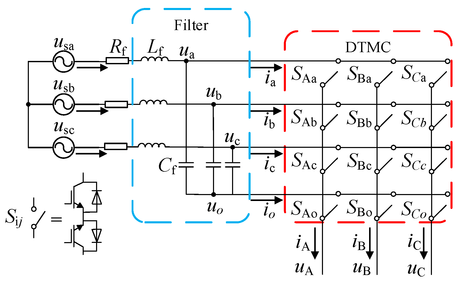
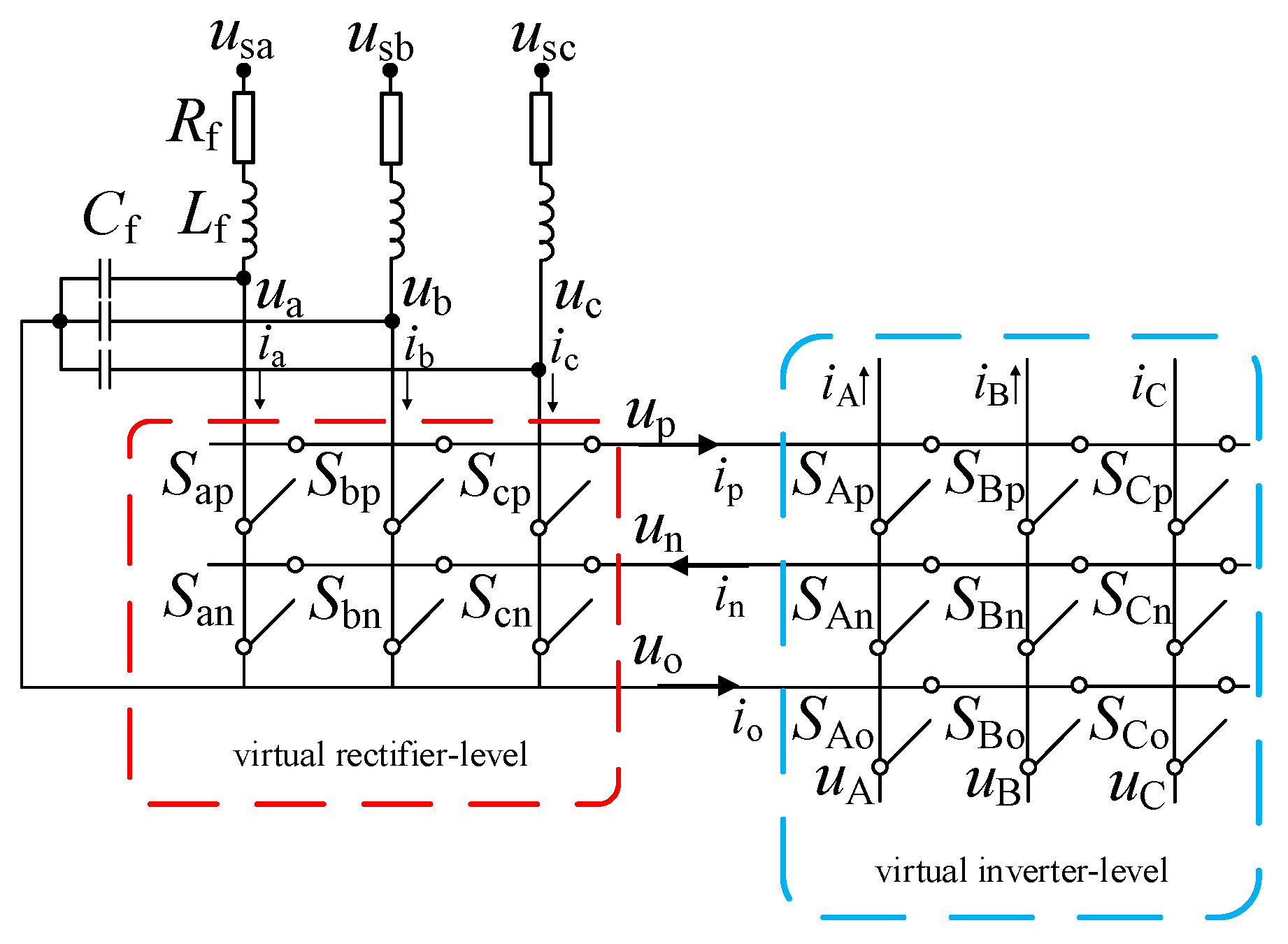
2. The Topology and Modulation Scheme of the DTMC

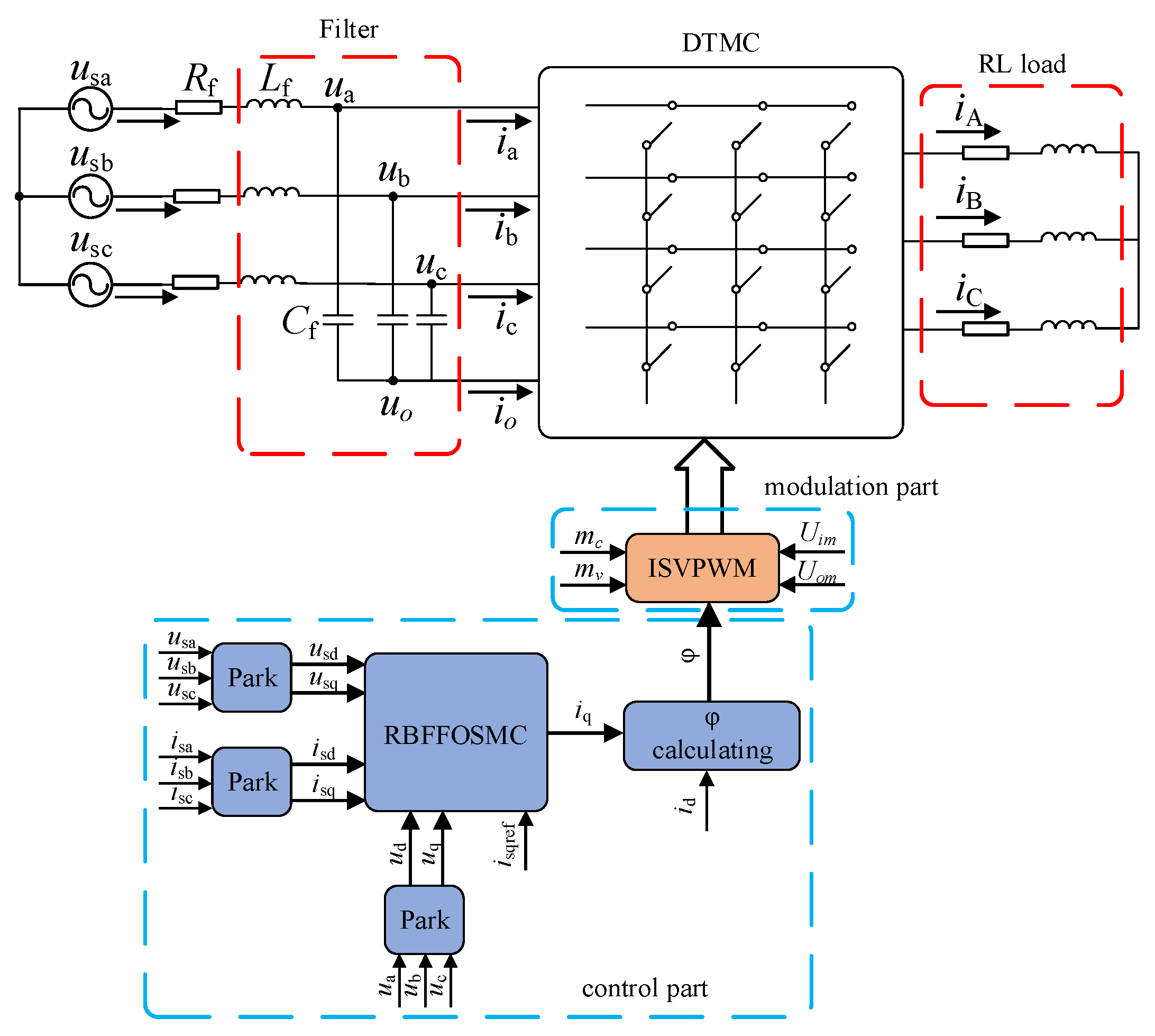
2.1. Topology of the DTMC

The DTMC topology is shown in Figure 1. It consisted of an array of 4 × 3 switches, which included the 3 × 3 switches of the conventional matrix converter and another three additional switches for the neutral point connection on the output side.

Each switch comprised two unidirectional controlled power semiconductor devices. The switches within the red dotted box In Figure 1 represent the DTMC. The input of the DTMC was composed of the voltage port, input filter, and damping resistor; the output usually connected to inductive load was a current port. The input filter (within the blue dotted box in Figure 1) contained the inductor, L_f. The film capacitor, C_f, was mainly used for filtering out the harmonics in the current.

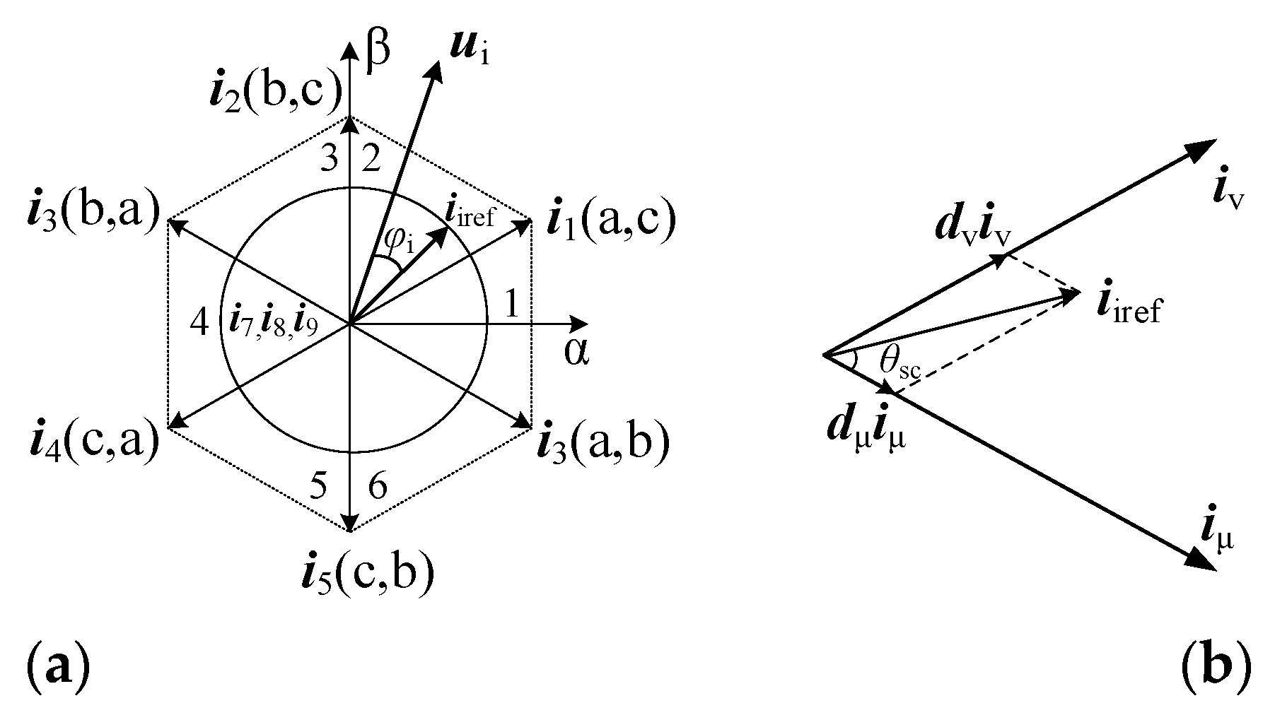
2.2. DTMC Modulation Algorithm

It can be seen from Figure 2 that the ISVPWM for the DTMC contained a virtual rectifier-level space vector modulation and a virtual inverter-level space vector modulation. The positive, neutral point, and negative terminals of the virtual inverter connected to u_p, u_n, and u_o of the intermediate virtual DC voltage.

The virtual rectifier-level space vector modulation of the DTMC used an input phase current modulation with a zero vector. Figure 3 shows the space vector modulation of a virtual rectifier. In Figure 3, u_i represents the space vector of the input phase voltage, φ_i represents the phase difference, and i_iref represents the space vector of the desired input phase current.

The duty cycles d_μ, d_ν, and d₀ of the effective vectors and zero vectors could be obtained according to the volt-second balance principle and the sinusoidal theorem:

$$\{\begin{array}{l}{d}_{\mu }=m_{\mathrm{c}}\sin \left({60}^{°}-{\theta }_{\mathrm{sc}}\right)\hfill \\ d_v=m_{\mathrm{c}}\sin \left({\theta }_{\mathrm{sc}}\right)\hfill \\ d_0=1-d_{\mu }-d_v\hfill \end{array}$$

(1)

$$m_{\mathrm{c}}=I_{\mathrm{im}}/i_{\mathrm{p},\mathrm{avg}}$$

(2)

where m_c is the input phase current space vector modulation factor and i_p,avg is the average value of the virtual DC link current.

In summary, the voltage and current of the virtual DC link were constant with a zero vector modulation in the local state averaging; the virtual inverter was powered by a constant DC source at the same time. Therefore, the modulation strategy of the virtual inverter stage was the same as a conventional inverter.

3. Instantaneous Power and Voltage Compensation under Unbalanced Grids

3.1. Instantaneous Power of the DTMC

When the three-phase voltage source failed, the input voltage and current could be expressed as (ignoring the zero-sequence component):

$$\{\begin{array}{c}{u}_{\mathrm{sa}}=U^{+}\cos \left({\omega }_{\mathrm{i}}t\right)+U^{-}\cos \left(-{\omega }_{\mathrm{i}}t-{\theta }^{-}\right)\\ u_{\mathrm{sb}}=U^{+}\cos \left({\omega }_{\mathrm{i}}t-2\pi /3\right)+U^{-}\cos \left(-{\omega }_{\mathrm{i}}t+2\pi /3-{\theta }^{-}\right)\\ u_{\mathrm{sc}}=U^{+}\cos \left({\omega }_{\mathrm{i}}t+2\pi /3\right)+U^{-}\cos \left(-{\omega }_{\mathrm{i}}t-2\pi /3-{\theta }^{-}\right)\end{array}$$

(3)

$$\{\begin{array}{c}{i}_{\mathrm{sa}}=I^{+}\cos \left({\omega }_{\mathrm{i}}t\right)+I^{-}\cos \left(-{\omega }_{\mathrm{i}}t-{\gamma }^{-}\right)\\ i_{\mathrm{sb}}=I^{+}\cos \left({\omega }_{\mathrm{i}}t-2\pi /3\right)+I^{-}\cos \left(-{\omega }_{\mathrm{i}}t+2\pi /3-{\gamma }^{-}\right)\\ i_{\mathrm{sc}}=I^{+}\cos \left({\omega }_{\mathrm{i}}t+2\pi /3\right)+I^{-}\cos \left(-{\omega }_{\mathrm{i}}t-2\pi /3-{\gamma }^{-}\right)\end{array}$$

(4)

where U⁺ (I⁺) and U⁻ (I⁻) are the amplitude of positive and negative sequence voltages (currents), respectively; ω_i represents the angular frequency; θ⁻ is the initial phase angle of the negative sequence voltage; and γ⁻ is the initial phase angle of the negative sequence voltage. The initial phase angle of the positive sequence voltage and current was assumed to be zero.

Combining Equations (3) and (4), the input instantaneous power of the DTMC was obtained.

$$\begin{array}{l}S=P_{\mathrm{s}}+\mathrm{j}{Q}_s\\ =\frac{3}{2}\left\{\begin{array}{l}{U}^{+}{I}^{+}\cos {\phi }^{+}+U^{-}{I}^{-}\cos \left({\gamma }^{-}-{\theta }^{-}\right)\hfill \\ +\left[U^{+}{I}^{-}\cos {\phi }^{-}+U^{-}{I}^{+}\cos {\theta }^{-}\right]\cos \left(2{\omega }_{\mathrm{i}}t\right)\hfill \\ +\left[-U^{+}{I}^{-}\sin {\phi }^{-}-U^{-}{I}^{+}\sin {\theta }^{-}\right]\sin \left(2{\omega }_{\mathrm{i}}t\right)\hfill \end{array}\right\}+\\ \mathrm{j}\frac{3}{2}\left\{\begin{array}{l}-U^{+}{I}^{+}\sin {\phi }^{+}-U^{-}{I}^{-}\sin \left({\gamma }^{-}-{\theta }^{-}\right)\hfill \\ +\left[U^{+}{I}^{-}\sin {\phi }^{-}+U^{-}{I}^{+}\sin {\theta }^{-}\right]\cos \left(2{\omega }_{i}t\right)\hfill \\ +\left[U^{+}{I}^{-}\cos {\phi }^{-}+U^{-}{I}^{+}\cos {\theta }^{-}\right]\sin \left(2{\omega }_{\mathrm{i}}t\right)\hfill \end{array}\right\}\\ =P_{\mathrm{s}0}+\underset{Secondharmonicof\mathrm{active}\mathrm{power}}{\underbrace{P_{\mathrm{s}2\sin }\cos (2\omega t)+P_{\mathrm{s}2\cos }\sin (2\omega t)}}+\\ Q_{\mathrm{s}0}+\underset{Secondharmonicof\mathrm{reactive}\mathrm{power}}{\underbrace{Q_{\mathrm{s}2\sin }\cos (2\omega t)+Q_{\mathrm{s}2\cos }\sin (2\omega t)}}\end{array}$$

(5)

where P_s (or Q_s) is the input active (or reactive) power, P_s0 and Q_s0 are the fundamental components of the input power, and P_s2 and Q_s2 are the second harmonics of the input power.

According to the principle of power conservation, by ignoring switching losses, the input power of the DTMC should equal the power consumed by the load. To ensure the balance of the three-phase output voltage, the second harmonic of the input power should be eliminated. Therefore, when the input voltage is unbalanced, the output voltage should be compensated.

3.2. Output Voltage Compensation

When the ISVPWM with a zero vector was used, the average of the virtual DC link voltage u_pn,avg during each cycle could be expressed as:

$$u_{\mathrm{pn},\mathrm{avg}}=\frac{3}{2}{m}_{\mathrm{c}}{U}_{\mathrm{im}}\cos {\phi }_{\mathrm{i}}.$$

(6)

From the virtual inverter-level modulation, the modulation coefficient could be expressed as:

$$m_{\mathrm{v}}=\sqrt{3}{U}_{\mathrm{om}}/u_{\mathrm{pn},\mathrm{avg}}$$

(7)

where U_om is the amplitude of the output voltage, U_im is the amplitude of the input voltage, and m_v is the space vector modulation factor of the output voltage.

When the input voltage was unbalanced, U_im and U_om were not constant, which led to unbalanced output voltages. Therefore, the value of m_v was adjusted according to Equation (7) to compensate for the output voltage and to achieve a balance.

4. RBF Neural Network Fractional-Order Sliding Mode Controller

4.1. Mathematical Models of the DTMC

According to Kirchhoff’s laws, the mathematical model of the DTMC on the input side (as shown in Figure 1 and Figure 2) could be obtained as:

$$\{\begin{array}{l}{u}_{\mathrm{sa}}-R_{\mathrm{f}}{i}_{\mathrm{sa}}-L_{\mathrm{f}}\frac{\mathrm{d}{i}_{\mathrm{sa}}}{\mathrm{d}t}-u_{\mathrm{a}}=0\hfill \\ u_{\mathrm{sb}}-R_{\mathrm{f}}{i}_{\mathrm{sb}}-L_{\mathrm{f}}\frac{\mathrm{d}{i}_{\mathrm{sb}}}{\mathrm{d}t}-u_{\mathrm{b}}=0\hfill \\ u_{\mathrm{sc}}-R_{\mathrm{f}}{i}_{\mathrm{sc}}-L_{\mathrm{f}}\frac{\mathrm{d}{i}_{\mathrm{sc}}}{\mathrm{d}t}-u_{\mathrm{c}}=0\hfill \end{array}$$

(8)

$$\{\begin{array}{l}{i}_{\mathrm{sa}}-C_{\mathrm{f}}\frac{\mathrm{d}{u}_{\mathrm{a}}}{\mathrm{d}t}-i_{\mathrm{a}}=0\hfill \\ i_{\mathrm{sb}}-C_{\mathrm{f}}\frac{\mathrm{d}{u}_{\mathrm{b}}}{\mathrm{d}t}-i_{\mathrm{b}}=0\hfill \\ i_{\mathrm{sc}}-C_{\mathrm{f}}\frac{\mathrm{d}{u}_{\mathrm{c}}}{\mathrm{d}t}-i_{\mathrm{c}}=0\hfill \end{array}$$

(9)

Transforming Equations (8) and (9) into dq coordinates, we could obtain:

$$\{\begin{array}{l}\frac{\mathrm{d}{i}_{\mathrm{sd}}}{\mathrm{d}t}=-\frac{R_{\mathrm{f}}}{L_{\mathrm{f}}}{i}_{\mathrm{sd}}+{\omega }_{\mathrm{i}}{i}_{\mathrm{sq}}+\frac{1}{L_{\mathrm{f}}}{u}_{\mathrm{sd}}-\frac{1}{L_{\mathrm{f}}}{u}_{\mathrm{d}}\hfill \\ \frac{\mathrm{d}{i}_{\mathrm{sq}}}{\mathrm{d}t}=-\frac{R_{\mathrm{f}}}{L_{\mathrm{f}}}{i}_{\mathrm{sq}}-{\omega }_{\mathrm{i}}{i}_{\mathrm{sd}}+\frac{1}{L_{\mathrm{f}}}{u}_{\mathrm{sq}}-\frac{1}{L_{\mathrm{f}}}{u}_{\mathrm{q}}\hfill \\ \frac{\mathrm{d}{u}_{\mathrm{d}}}{\mathrm{d}t}=\frac{1}{C_{\mathrm{f}}}{i}_{\mathrm{sd}}+{\omega }_{\mathrm{i}}{u}_{\mathrm{q}}-\frac{1}{C_{\mathrm{f}}}{i}_{\mathrm{d}}\hfill \\ \frac{\mathrm{d}{u}_{\mathrm{q}}}{\mathrm{d}t}=\frac{1}{C_{\mathrm{f}}}{i}_{\mathrm{sq}}-{\omega }_{\mathrm{i}}{u}_{\mathrm{d}}-\frac{1}{C_{\mathrm{f}}}{i}_{\mathrm{q}}\hfill \end{array}$$

(10)

where u_sj and i_sj (j = a, b, c, d, q) represent the grid voltages and grid currents, respectively; u_j and i_j are the input voltage and current of the DTMC, respectively; and R_f is the damping resistor.

To ensure that the grid voltage and current could achieve a unity power factor, we controlled the impedance angle. The impedance angle could be described as:

$${\phi }_{\mathrm{i}}=\arctan \left(\frac{i_{\mathrm{q}}}{i_{\mathrm{d}}}\right).$$

(11)

To ensure the reliability of the electricity, when the reference signals of the reactive power changes, the active power should be stable. Therefore, from Equation (11), the impedance angle could be controlled by i_q, which could ensure that the active power was constant. The input side of the DTMC based on the q-axis could be described as:

$$\frac{\mathrm{d}{i}_{\mathrm{sq}}}{\mathrm{d}t}=-\frac{R_{\mathrm{f}}}{L_{\mathrm{f}}}{i}_{\mathrm{sq}}-{\omega }_{\mathrm{i}}{i}_{\mathrm{sd}}+\frac{1}{L_{\mathrm{f}}}{u}_{\mathrm{sq}}-\frac{1}{L_{\mathrm{f}}}{u}_{\mathrm{q}}$$

(12)

$$\frac{\mathrm{d}{u}_{\mathrm{q}}}{\mathrm{d}t}=\frac{1}{C_{\mathrm{f}}}{i}_{\mathrm{sq}}-{\omega }_{\mathrm{i}}{u}_{\mathrm{d}}-\frac{1}{C_{\mathrm{f}}}{i}_{\mathrm{q}}.$$

(13)

From a derivative of Equation (12) and a combination with Equation (10), we could obtain:

$$\begin{array}{ll}\frac{{\mathrm{d}}^2{i}_{\mathrm{sq}}}{\mathrm{d}{t}^2}=& {\omega }_{\mathrm{r}}^2{i}_{\mathrm{q}}-\frac{R_{\mathrm{f}}}{L_{\mathrm{f}}}\frac{\mathrm{d}}{\mathrm{d}t}{i}_{\mathrm{sq}}\\ & -{\omega }_{\mathrm{r}}^2{i}_{\mathrm{sq}}-{\omega }_{\mathrm{i}}\frac{\mathrm{d}}{\mathrm{d}t}{i}_{\mathrm{sd}}+\frac{1}{L_{\mathrm{f}}}\frac{\mathrm{d}}{\mathrm{d}t}{u}_{\mathrm{sq}}+\frac{{\omega }_{\mathrm{i}}}{L_{\mathrm{f}}}{u}_{\mathrm{d}}\end{array}$$

(14)

where ${\omega }_{\mathrm{r}}^2=1/\left(L_{\mathrm{f}}{C}_{\mathrm{f}}\right)$.

4.2. Fractional-Order SMC

The order of calculus is usually an integer order. The fractional-order calculus extends the calculus procedures to a more general form in which the order of the derivative is a fraction.

The fractional-order calculus is defined as:

$${}_a{D}_t^{\alpha }\{\begin{array}{ll}\frac{d^{\alpha }}{d{t}^{\alpha }}\hfill & \alpha >0\hfill \\ 1\hfill & \alpha =0\hfill \\ {\displaystyle {\int }_a^t{(d\tau )}^{\alpha }}\hfill & \alpha <0\hfill \end{array}$$

(15)

where ${ }_a{D}_t^{\mathsf{\alpha }}$ is the symbol of the fractional-order calculus, a and t are the upper and lower boundaries of the operation, and α is the order of the fractional-order calculus, respectively.

We used the Caputo fractional-order for the proposed control method. The Caputo fractional-order was defined as:

$$D^{\alpha }f(t)=\frac{1}{\mathsf{\Gamma }(n-\alpha )}{\displaystyle {\int }_0^t\frac{f^{(n)}(\tau )}{{(t-\tau )}^{\alpha -n+1}}}d\tau ,n-1<\alpha <n$$

(16)

where Γ (·) is a gamma function, Γ$(\gamma )={\int }_0^{\infty }{e}^{-t}{t}^{\gamma -1}dt$, and n is a positive integer. Here, n = 1.

Defining $x_1=i_{sq}$ and $x_2=\frac{\mathrm{d}{i}_{sq}}{\mathrm{d}t}$, Equation (14) could be transformed into a state-space representation:

$$\{\begin{array}{l}{\dot{x}}_1=x_2\hfill \\ {\dot{x}}_2=x_1\left(\frac{R_{\mathrm{f}}^2}{L_{\mathrm{f}}^2}-{\omega }_{\mathrm{i}}^2-{\omega }_{\mathrm{r}}^2\right)+i_{\mathrm{sd}}\left(\frac{2{\omega }_{\mathrm{i}}{R}_{\mathrm{f}}}{L_{\mathrm{f}}}\right)-u_{\mathrm{sd}}\left(\frac{{\omega }_{\mathrm{i}}}{L_{\mathrm{f}}}\right)\hfill \\ -u_{\mathrm{sq}}\left(\frac{R_{\mathrm{f}}}{L_{\mathrm{f}}^2}\right)+u_{\mathrm{d}}\left(\frac{2{\omega }_{\mathrm{i}}}{L_{\mathrm{f}}}\right)+u_{\mathrm{q}}\left(\frac{R_{\mathrm{f}}}{L_{\mathrm{f}}^2}\right)+\frac{1}{L_{\mathrm{f}}}\frac{\mathrm{d}{u}_{\mathrm{sq}}}{\mathrm{d}t}+{\omega }_{\mathrm{r}}^2{i}_{\mathrm{q}}\hfill \end{array}$$

(17)

The reference current of the q-axis was defined as i_sqref and the current tracking error was defined as $e=i_{\mathrm{sqref}}-i_{\mathrm{sq}}=x_{1\mathrm{ref}}-x_1$.

We defined the fractional-order sliding surface as:

$$s=c_1{D}^{1-\mu }e+c_{2}e+c_3{D}^{\alpha -1}e$$

(18)

where c₁ and c₂ are constants, D^α−1e is the α − 1 order integration of the error, D^1−μe is the 1 − μ order derivative of the error, 0 < α, and μ < 1.

To compensate for the effect of the lumped uncertainties, we designed an exponential reaching law as follows.

In order to reduce the high frequency jitter of the SMC, the saturation function, sat (·), was used instead of the sign function, sgn (·), in the ideal sliding mode (called the quasi-sliding mode). The exponential reaching law was designed as follows:

$$\dot{s}(t)=-\epsilon \mathrm{sgn}(s(t))-qs(t)=-\epsilon sat(s(t))-qs(t)$$

(19)

where ε and q are positive constants.

From a derivative of Equation (18) and a combination with Equation (19), we could obtain:

$$\begin{array}{ll}{c}_1{D}^{2-\mu }e+c_2\dot{e}+c_3{D}^{\alpha }e& =c_1{D}^{-\mu }\ddot{e}+c_2\dot{e}+c_3{D}^{\alpha }e\\ & =-\epsilon sat(s(t))-qs(t)\end{array}$$

(20)

By substituting Equation (20) into Equation (17), the following FOSMC control law of the q-axis current was obtained:

$$i_q=\frac{1}{{\omega }_{\mathrm{r}}^2}\left[\begin{array}{c}{i}_{sq}\left({\omega }_{\mathrm{i}}^2+{\omega }_{\mathrm{r}}^2-\frac{R_{\mathrm{f}}^2}{L_{\mathrm{f}}^2}+K_1\frac{R_{\mathrm{f}}}{L_{\mathrm{f}}}-K_2\right)+\\ i_{\mathrm{sd}}\left(-\frac{2R_{\mathrm{f}}}{L_{\mathrm{f}}}+K_1{\omega }_{\mathrm{i}}\right)+u_{\mathrm{sd}}\frac{{\omega }_{\mathrm{i}}}{L_{\mathrm{f}}}+u_{\mathrm{sq}}\left(\frac{R_{\mathrm{f}}}{L_{\mathrm{f}}^2}-\frac{K_1}{L_{\mathrm{f}}}\right)\\ +u_d\left(\frac{-2\omega }{L}\right)+u_{\mathrm{q}}\left(-\frac{R_{\mathrm{f}}}{L_{\mathrm{f}}^2}+\frac{K_1}{L_{\mathrm{f}}}\right)+K_2{i}_{\mathrm{sqref}}\\ +q\frac{c_3{D}^{a-1}}{c_2}\left(i_{\mathrm{sqref}}-i_{\mathrm{sq}}\right)+\frac{\epsilon }{c_1{D}^{-\mu }}sat(S(t))\end{array}\right]$$

(21)

where $K_1=\frac{c_2}{c_1{D}^{-\mu }}+q$ and $K_2=\frac{c_3{D}^a}{c_1{D}^{-\mu }}+q\frac{c_2}{c_1{D}^{-\mu }}$.

It can be seen from Equation (21) that the FOSMC control law contained the device parameters R_f, L_f, C_f, and ω_i and the controller parameters c₁, c₂, c₃, ε, q, α, and μ. However, parametric variations caused by aging inductors and capacitors are a nonlinear function and ω_i is related to the grid frequency in practical applications. In addition, it can be difficult to adjust the controller parameters. Therefore, an RBF NN was proposed to fit Equation (21). The nonlinear function was described as:

$$i_q=\mathrm{F}\left(i_{sq},i_{\mathrm{sd}},u_{\mathrm{sd}},u_{\mathrm{sq}},u_d,u_q,s\right).$$

(22)

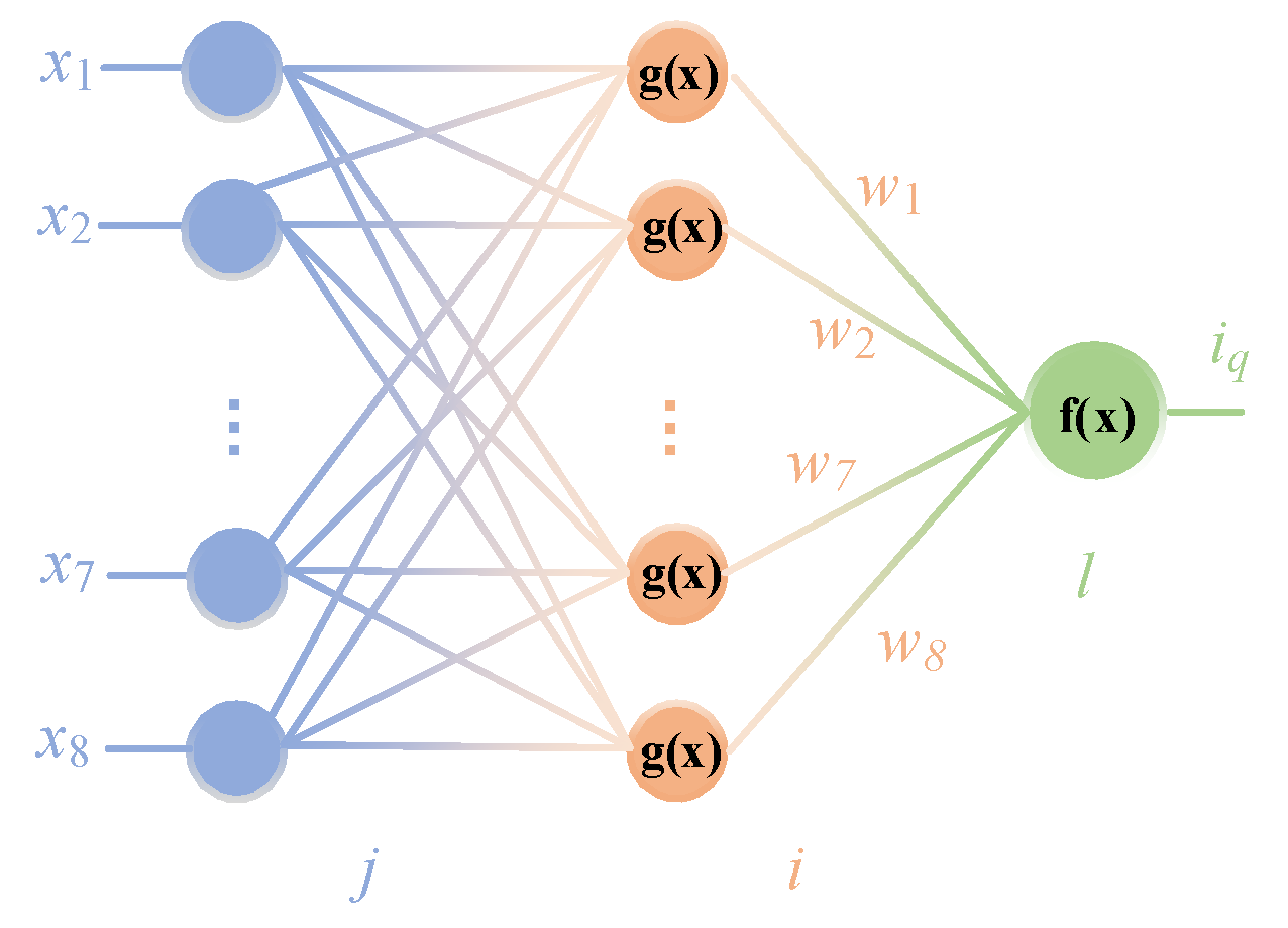
4.3. RBF Neural Network

The input layer, hidden layer, and output layer are the three layers of a forwarding structure in an RBF NN. A basic RBF NN is shown in Figure 4.

As shown in Figure 4, the input of the RBF NN was:

$$x={\left[x_1,x_2,\dots x_j\right]}^{\mathrm{T}},j=1,2,\dots ,7.$$

(23)

The output of the input layer was:

$$O_j^{(1)}=x(j),j=1,2,...,7.$$

(24)

The input of the hidden layer was:

$${\mathrm{net}}_i^{(2)}=x,x=(x(1),x(2),.....,x(7)).$$

(25)

The output of the hidden layer was:

$$O_i^{(2)}(k)=g\left({\mathrm{net}}_i^{(2)}(k)\right),i=1,2\dots 8.$$

(26)

To distinguish across the layers, superscripts ¹, ², and ³ were used to denote the input, hidden, and output layers, respectively. The Gauss function was g(x).

$$g(x)=\exp \left(-\frac{{\Vert x-c_i\Vert }^2}{2b_i^2}\right)$$

(27)

where $c_i=\left[c_{i1},\dots ,c_{in}\right]$, which was the center vector of the ith hidden layer neuron. The width vector of the Gauss function was $b_i={\left[b_1,b_2,\dots ,b_m\right]}^{\mathrm{T}}$.

The input of the NN output layer was:

$${\mathrm{net}}_i^{(3)}(k)={\displaystyle \sum _{i=1}^8{w}_i^{(3)}}{O}_i^{(2)}(k).$$

(28)

The output of the NN was as follows:

$$i_q=O_i^{(3)}(k)=f\left({\mathrm{net}}_l^{(3)}(k)\right),l=1$$

(29)

where $w_{li}^{\left(3\right)}$ is the weight of the hidden layer to the output layer. The activation function of the output layer was:

$$f(x)=\frac{e^x}{e^x+e^{-x}}.$$

(30)

The performance function of this NN was as follows:

$$E(k)=\frac{1}{2}{\left(i_{\mathrm{qref}}-i_q\right)}^2$$

(31)

where i_qref is the set value of i_q, which was related to the reactive power. In this article, i_qref = 0.

The network weight was adjusted using the gradient descent approach. An inertia term was included in the formula to improve the convergence speed.

$$\mathsf{\Delta }{w}_{li}^{(3)}(k)=-\eta \frac{\partial E(k)}{\partial w_{li}^{(3)}}+\alpha \mathsf{\Delta }{w}_{li}^{(3)}(k-1)$$

(32)

where η is the learning rate and α is the inertial coefficient.

In summary, the weight adjustment formula of the RBF NN was Equation (32) and the parameters and the number of neurons was as follows.

(1) Number of neurons: When the control system was confirmed, the number of the input and output neurons was also determined. In this paper, the input and output layers w 2 and 1, respectively. There is no currently no uniform formula to determine the number of middle layer neurons. According to

Table 1. MSE with different number of neurons.

Number of Neurons in the Middle Layer	4	8	16
MSE	3.336 × 10−5	1.0259 × 10−6	5.0258 × 10−6

and Figure 5, the best results were obtained when the number of neurons in the middle layer was 8. The input and output layers were 2 and 1, respectively.

(2) Parameter Setting: The settings of a_i and b_i also affected the output of the RBF NN. When the input was close to a_i, the value of the Gauss function was sensitive and b_i was the mapping range of the Gauss function. In this paper, a_i was 0 and b_i was 1.

5. Simulation and Experiment Results

5.1. Simulation

To show the validity of the suggested controller, we built a model in MATLAB/Simulink according to Figure 6. The parameters of the simulation are listed in

Table 2. Simulation parameters.

Parameters	Values
Grid voltage usj/V	311
Filter capacitors Cf/μF	12
Filter inductors Lf/mH	2
Damping resistors Rf/Ω	2
Load resistors RL/Ω	10
Load inductors Lf/mH	10
Output frequency f0/Hz	25
Active power Pref/W	5000
Modulation factor mc, mv	0.8, 0.9
RBF hidden layer nodes	8
Learning rate η	0.5
Inertial coefficient α	0.05
Switching frequency fs/kHz	20

. The average reactive power reference was set to zero (Q_ref = 0).

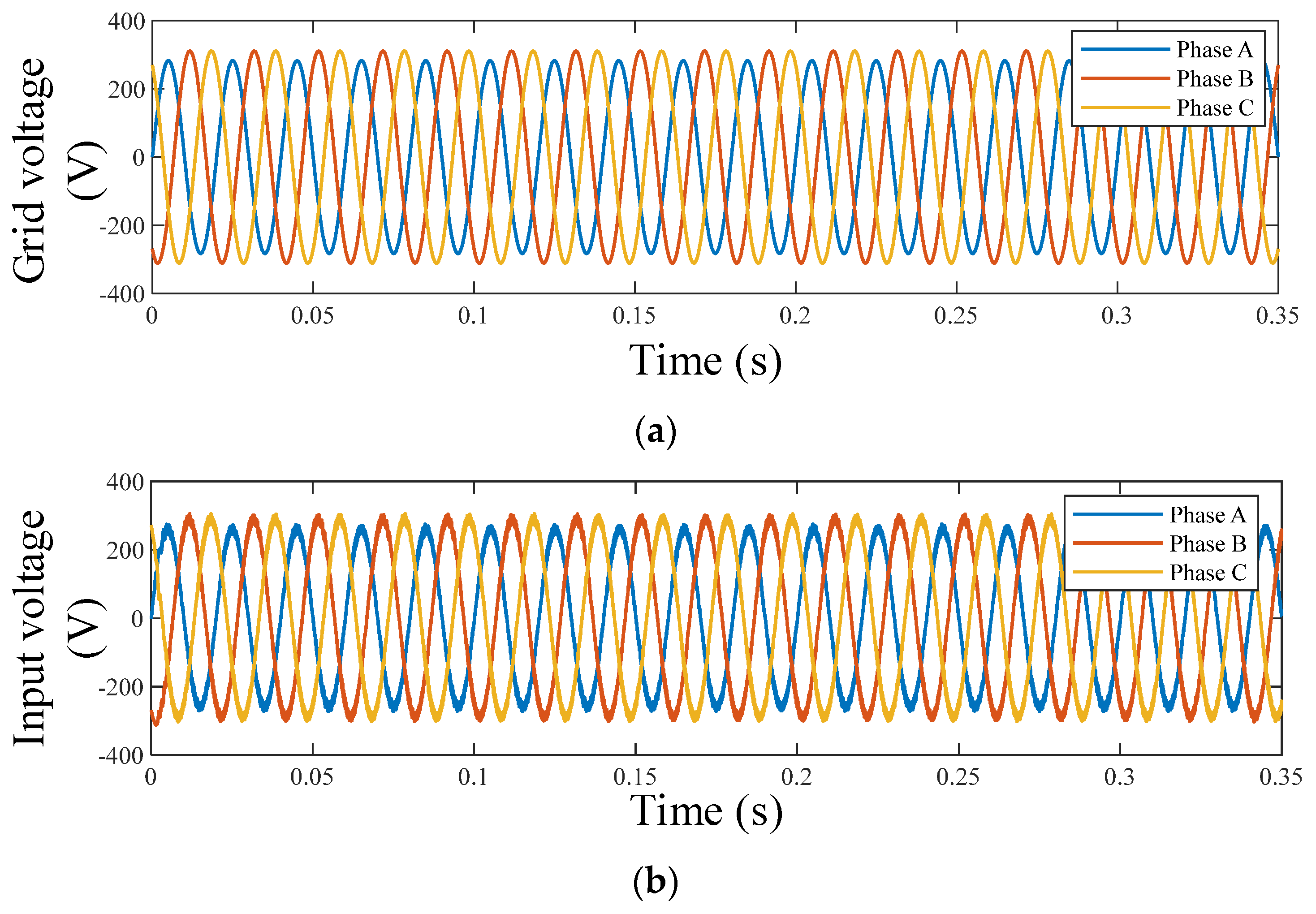
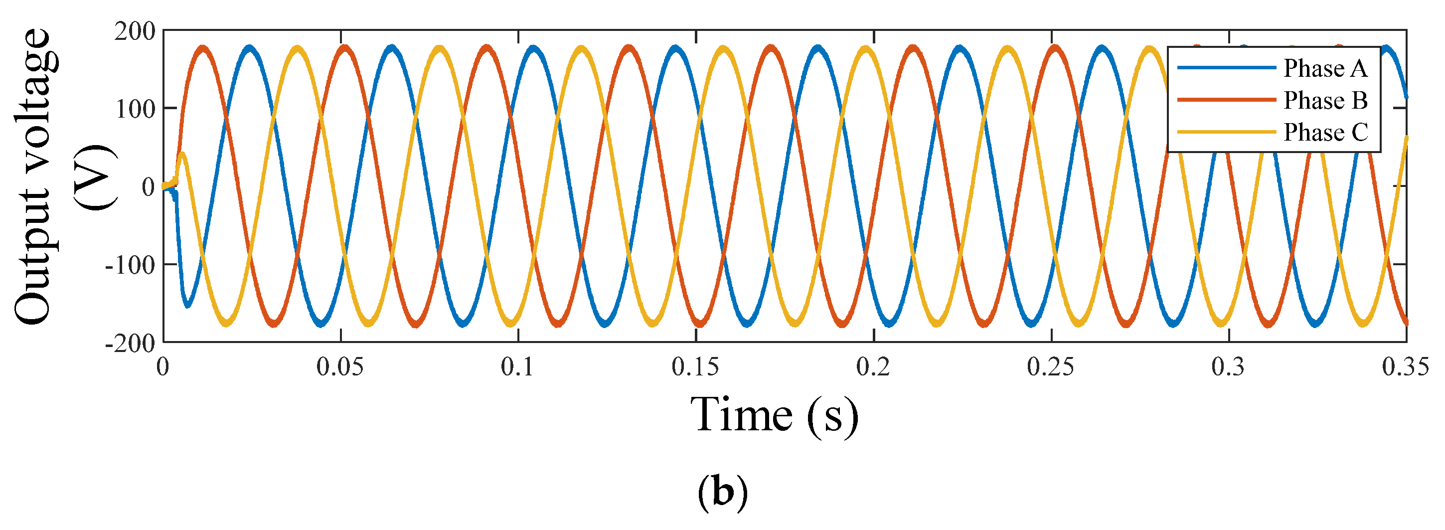
5.1.1. Imbalance Analysis

As shown in Figure 7a, the performance of the suggested control method was assessed with a 10% reduction in the phase amplitude. The nonlinear loads connected to the grid led to distortions observed in the grid voltage waveforms. Figure 7b shows the waveforms of the DTMC input voltage. We observed that the high switching frequency current harmonics flowing into the filter capacitors were the primary cause of high frequency distortion.

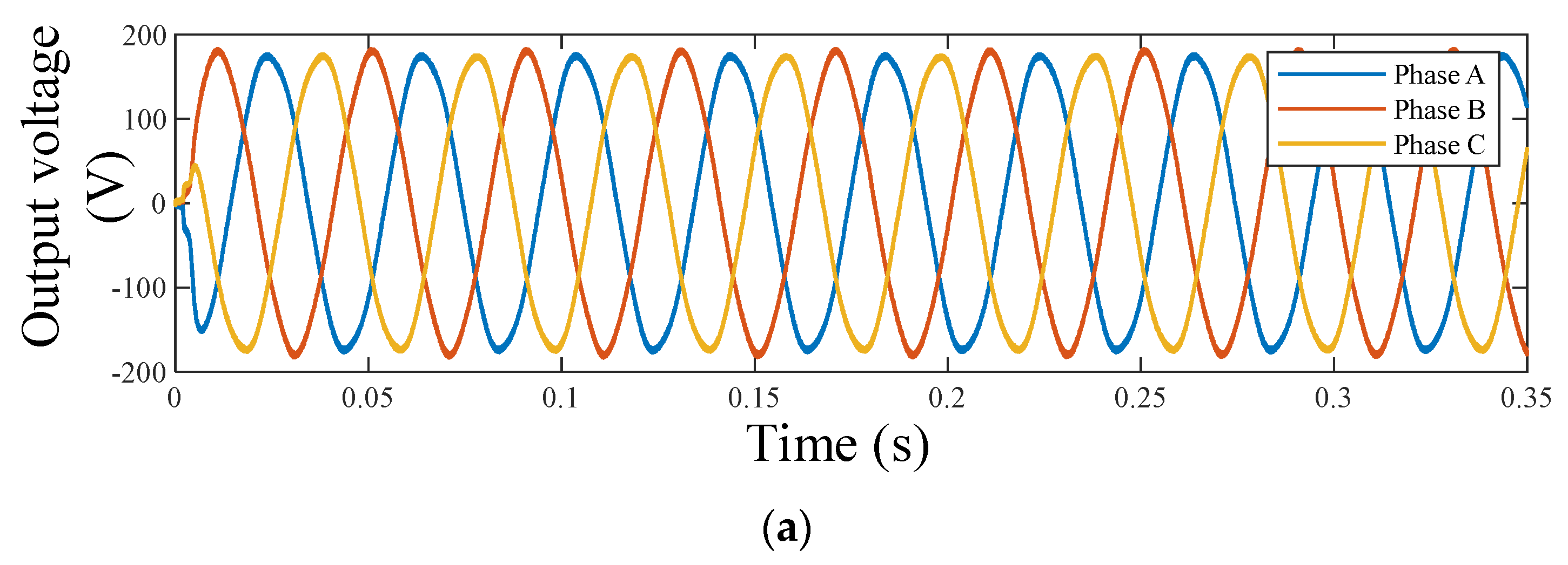
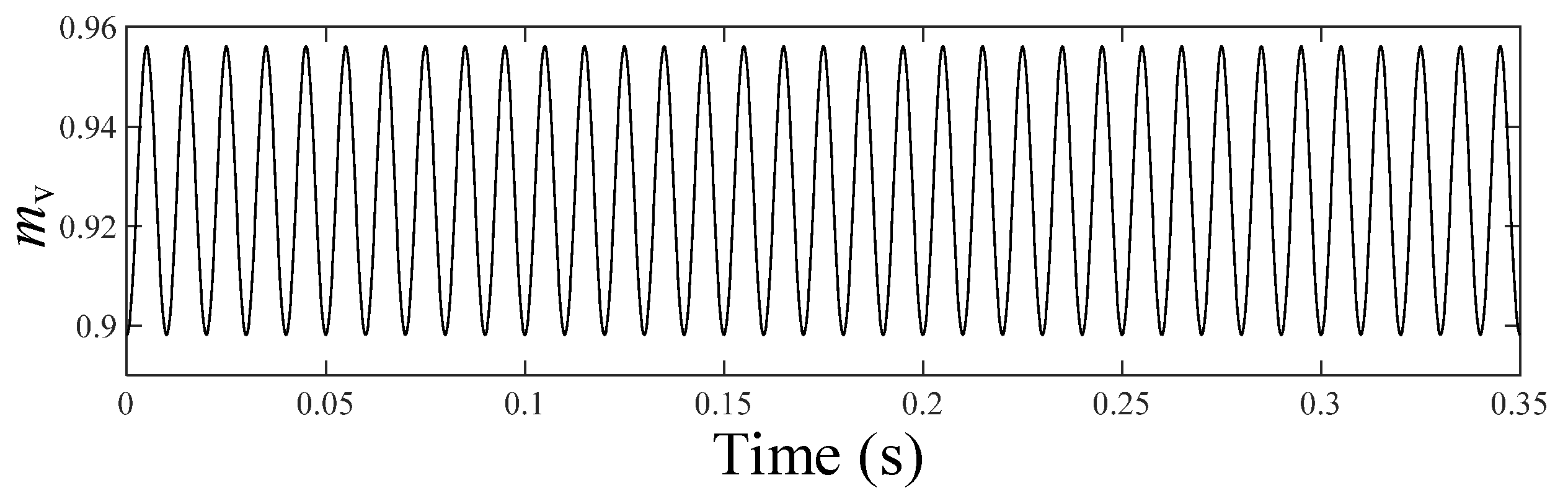
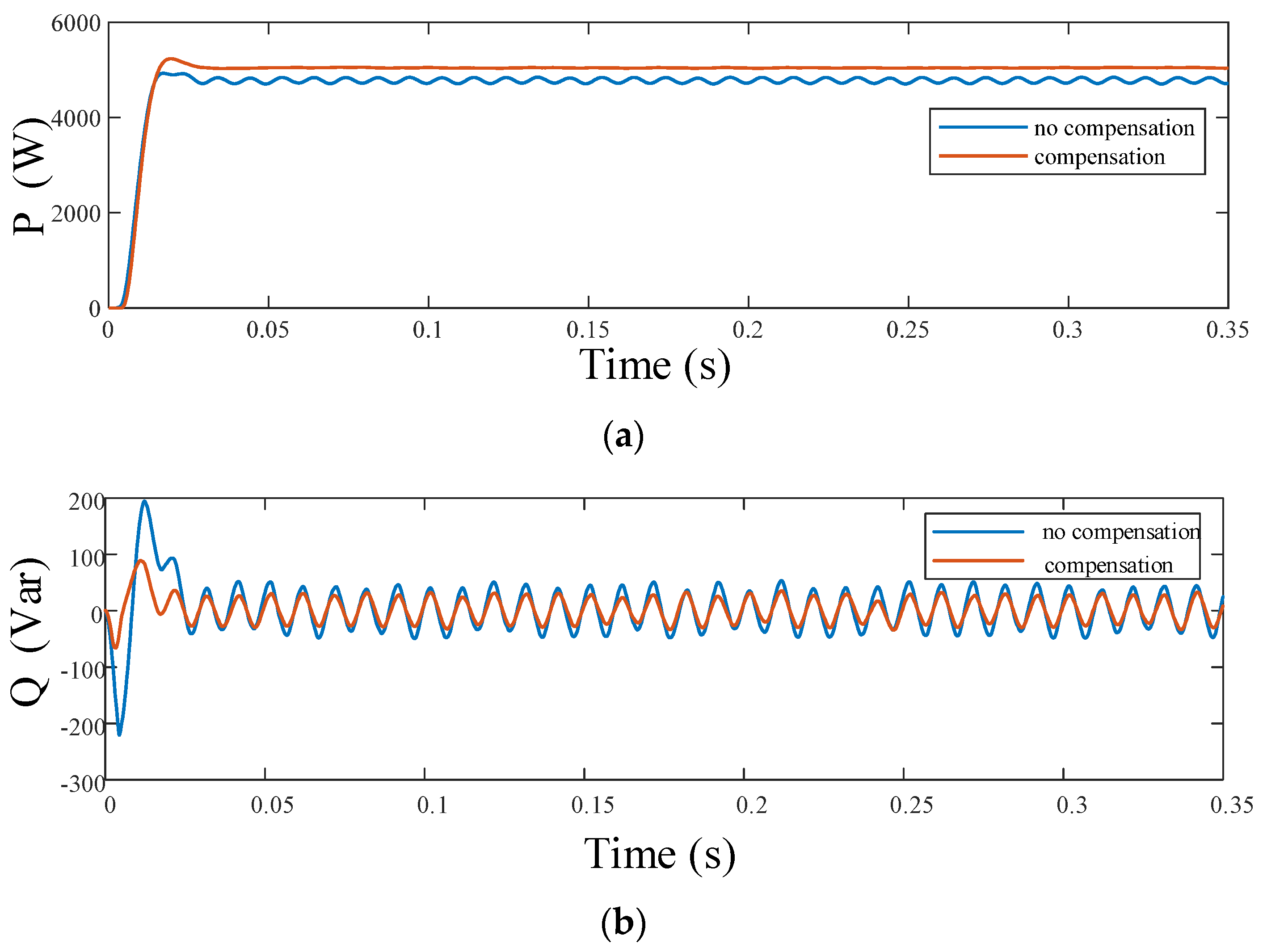
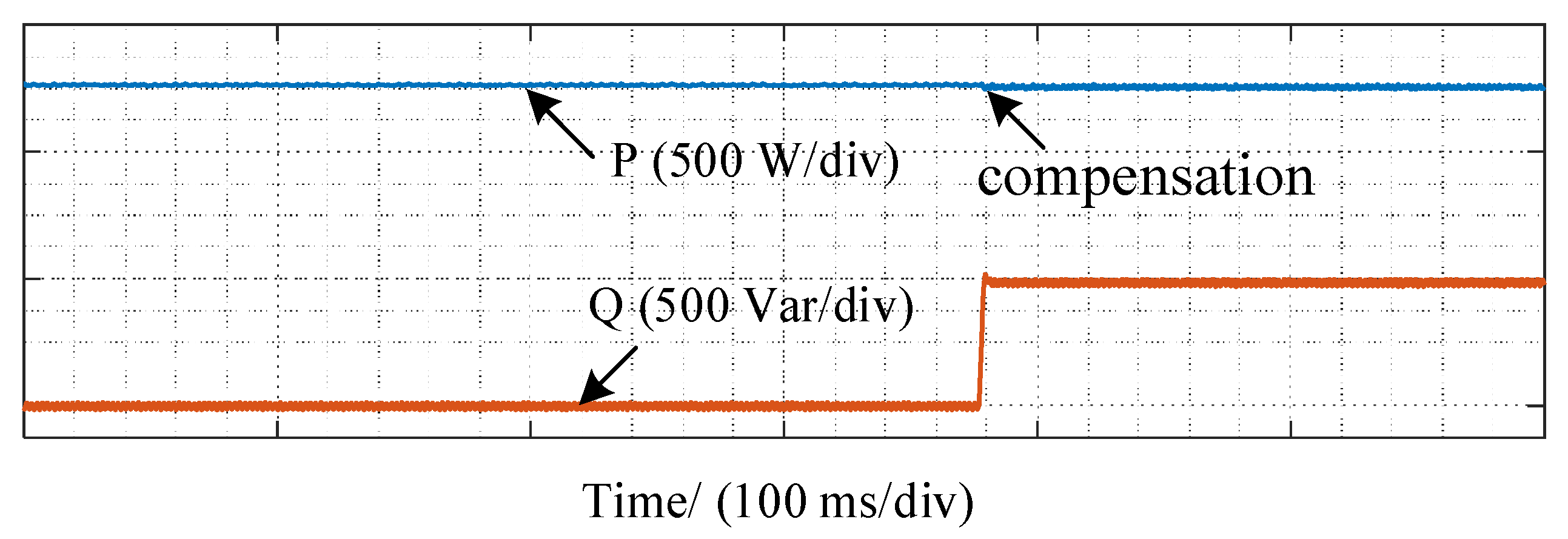
5.1.2. Output Compensation Analysis

Figure 8a,b illustrates the output voltage fundamental waveform of the DTMC. The cut-off frequency of the filter was 50 Hz. Although the grid voltage was imbalanced, the DTMC could produce three-phase balanced and sinusoidal voltages after the voltage compensation proposed in the article, as shown in Figure 8b. Conversely, the uncompensated waveform suffered from three-phase imbalance and distortion.

Figure 9 shows the waveform of the output voltage modulation coefficient, m_v. From Figure 8, it can be seen that m_v fluctuate between 0.9 and 0.96. When the input voltage amplitude was at maximum, m_v was minimum so the output voltage could reach a balance, which was consistent with the theoretical analysis of Section 3.2.

Figure 10a,b illustrates the power waveform of the DTMC. In Figure 10a, it can be seen that there were twice the frequency components and active power drops with no compensation. According to Section 3, the output active power was a constant value after compensation. It can be seen in Figure 10b that the overshoot and fluctuations of the reactive power were smaller after compensation.

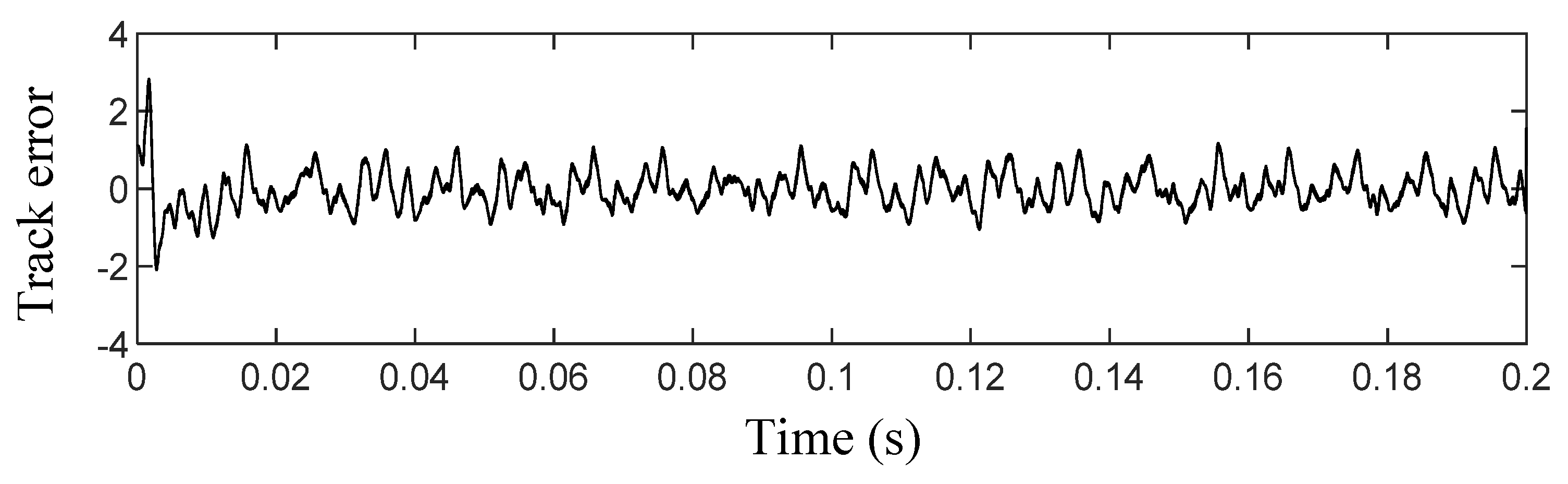
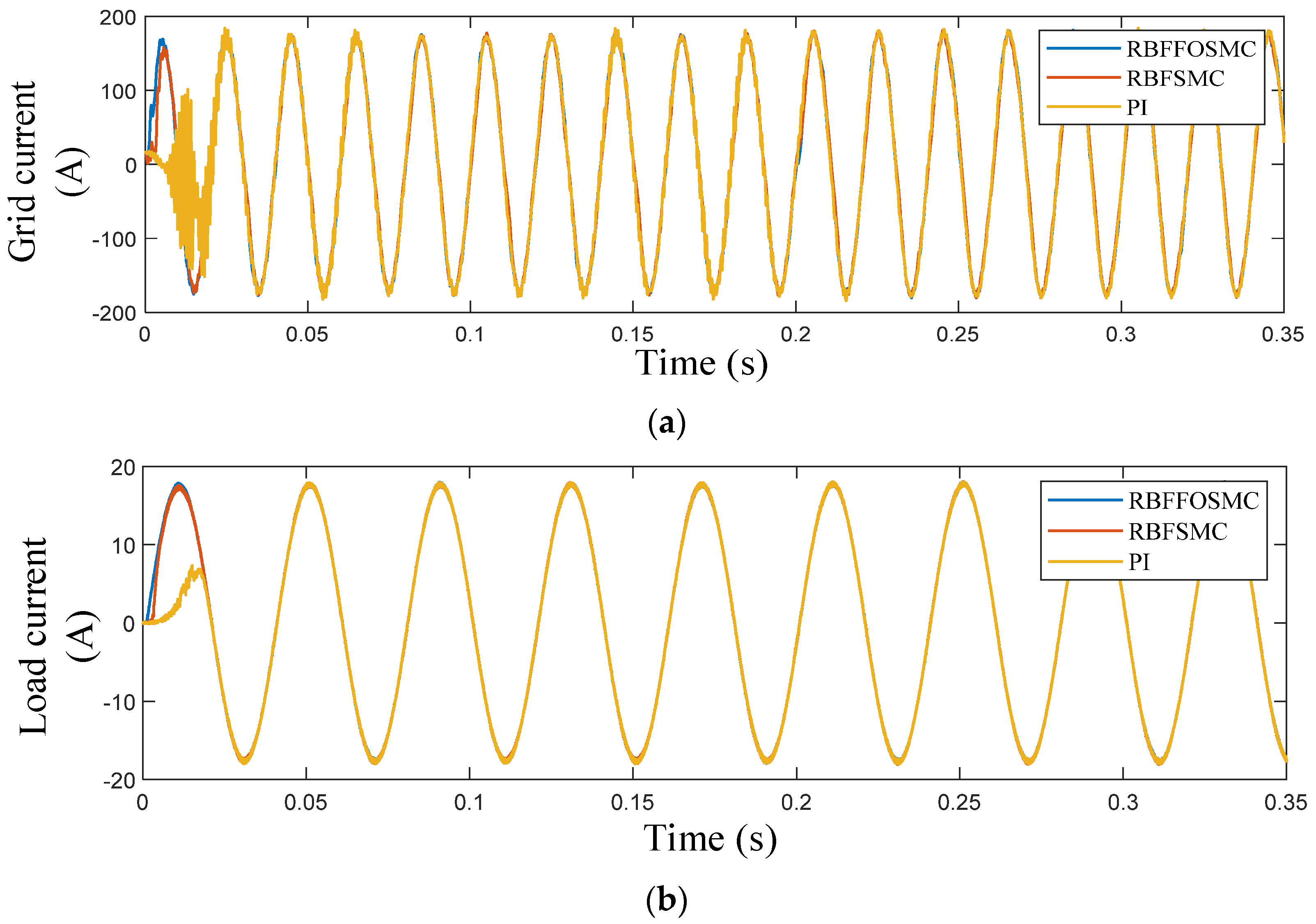
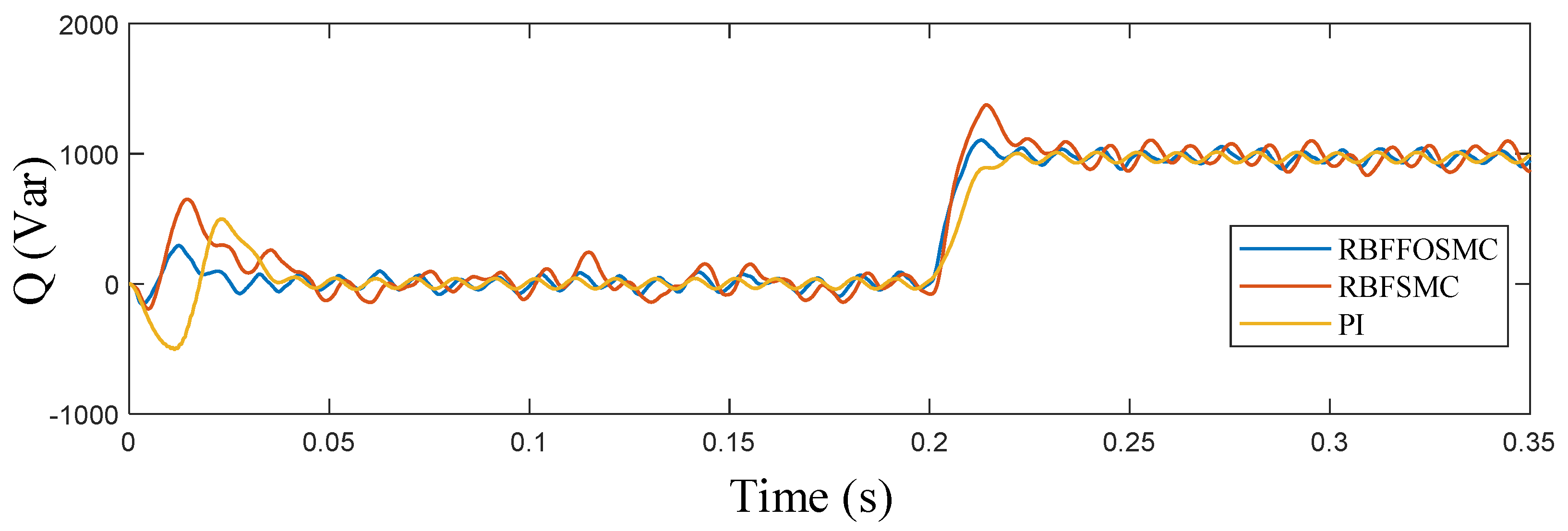
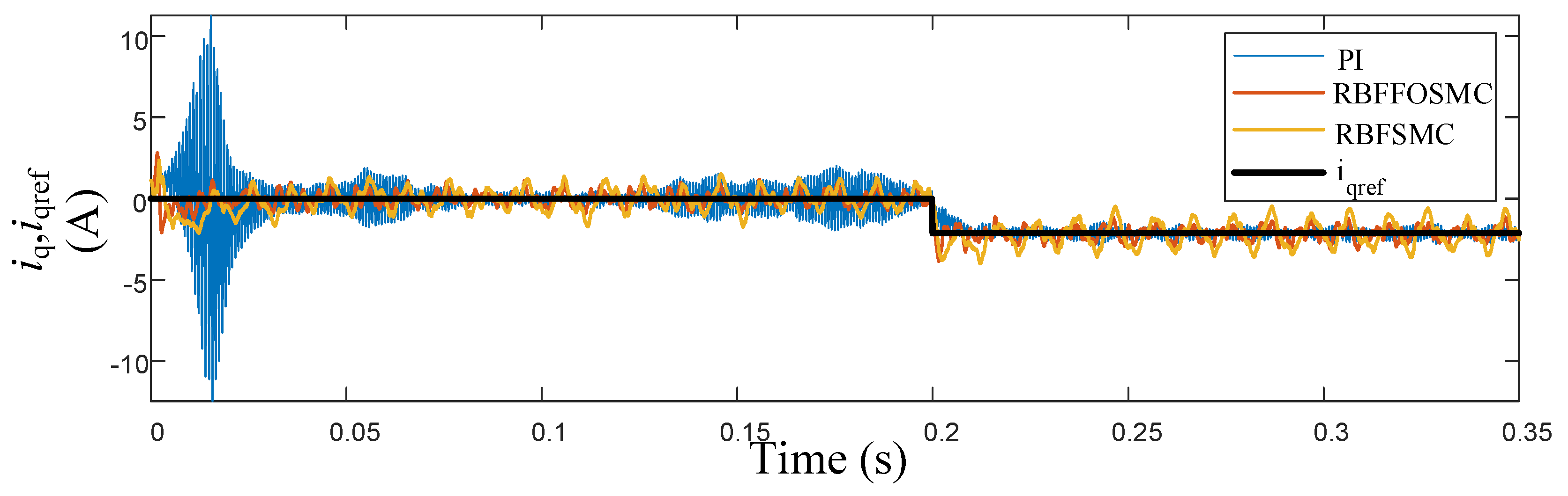
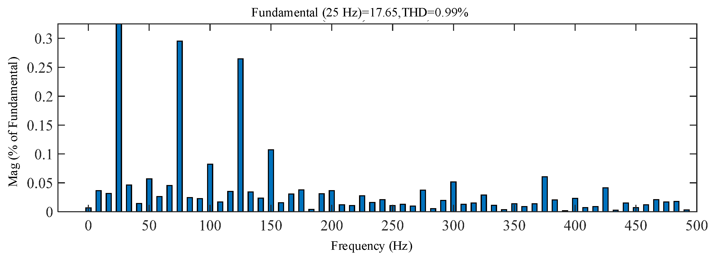
5.1.3. Controller Performance Analysis

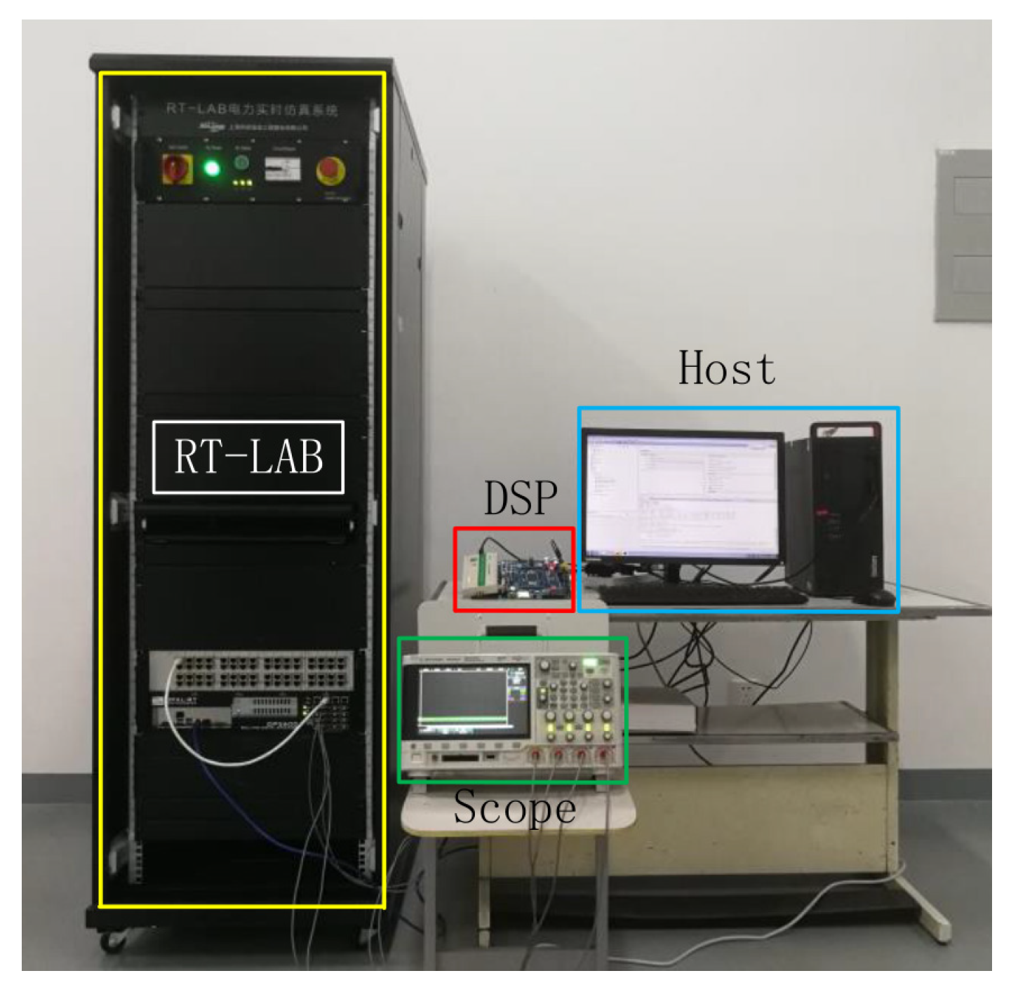
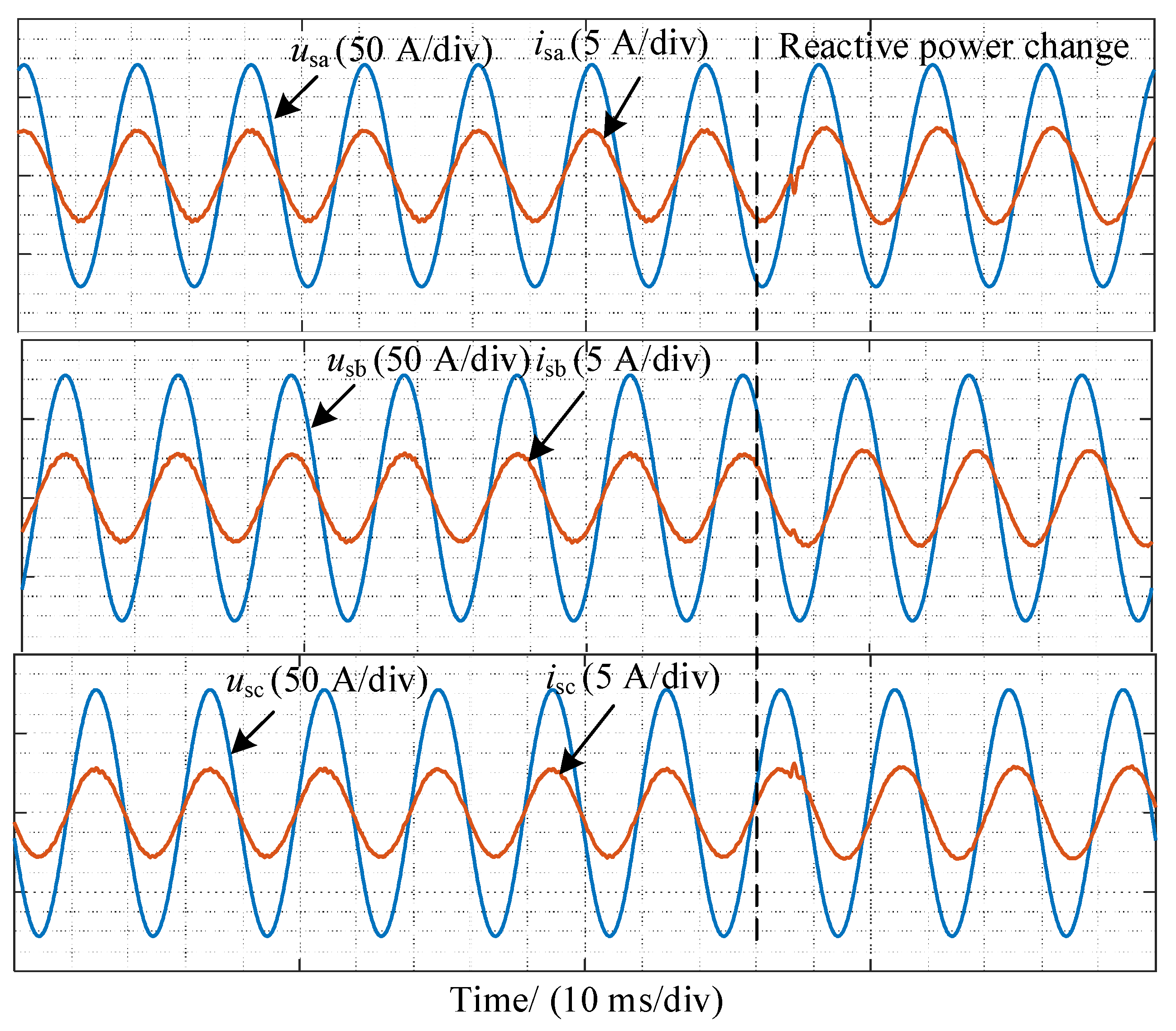
To verify the effectiveness of the controller proposed in the article, the reactive power was increased abruptly from 0 var to 1000 var at 0.2 s and was compared with a conventional PI control as well as a sliding mode controller based on an RBF NN (RBFSMC).

Figure 11 shows the grid and load current of phase A. As can be seen in Figure 11, the RBFFOSMC took about 0.005 s to reach stability by the controller proposed in the article, which was better than the PI control and RBFSMC. The load currents had an excellent dynamic and steady performance under the RBFFOSMC. When the set value changed suddenly, the output current did not fluctuate at 0.2 s. The PI control took about 30 ms and the RBFSMC took about 5 ms to become stable whereas the RBFFOSMC immediately reached stability.

Table 3. FFT analysis of grid current of Phase A.

Grid Side Current	RBFFOSMC	RBFSMC	PI
FFT Analysis	2.29%	5.46%	5.66%

shows the FFT analysis of the grid current of Phase A. As can be seen in Table 3, the FFT was over 5% under the RBFSMC and PI control. According to IEEE Std 519, the FFT of the grid current should be less than 5%. The FFT under the RBFSMC fulfilled this requirement.

Figure 12 shows the reactive power controlled by the RBFFOSMC, RBFSMC, and PI control. When the reactive power rose at 0.2 s, the proposed controller in this article could immediately track the set value whereas the overshoot was larger and the setting time was longer when controlled by the PI control and the RBFSMC. Figure 13 shows the tracking performance of i_q. It could track the i_qref without any delay whereas it took about 20 ms under the PI control and 10 ms under the RBFSMC to track the i_qref. In addition, i_q fluctuated more frequently under the PI controller at 0 s.

5.2. Experiment

In this paper, the hardware in the loop simulation platform based on an RT-LAB was built. This platform included a DSPTMS32F28335 as the main control device and RT-LAB equipment was used to build the hardware model. The platform is shown in Figure 14.

The RT-LAB obtained a PWM control signal from the DSP, which was the gate signal of the IGBT in the DTMC. Each converter output the voltage and current under the control of the corresponding PWM signal. The switching frequency of the IGBT was 20 kHz. According to Shannon’s theorem, the sampling frequency must be greater than 40 kHz. In this experiment, the sampling frequency was set to 1 MHz. The experimental parameters were consistent with the simulation.

As shown in Figure 15, as with the simulation, the amplitude of u_sa decreased by 10%. The line currents remained sinusoidal and in phase with their corresponding grid voltages. Therefore, the unity input power factor operation was also achieved before the reactive power changes. When the grid voltage was imbalanced, the converter was required to inject reactive power into the grid. In order to ensure the reliability of the power supply, when the reactive power changed, the active power should not change. As a result, the active power needed to be compensated and the output of the converter was no longer a unit power factor. These results confirmed that the RBFFOSMC and voltage compensation operated perfectly even under these unfavorable conditions of grid voltages.

The load current illustrated in Figure 16 shows clearly that converter was also able to provide balanced currents to the load despite the imbalanced grid. There were no fluctuations when the reactive power changed, which guaranteed the reliability of the power on the load side. In addition, an FFT analysis of the load current of phase A was performed by MATLAB. The result is shown in Figure 17. This value was close to the simulation result, which verified the validity of the simulation. The DTMC could output perfect waveforms under the proposed controller.

Figure 18 shows the active and reactive power waveforms. It could be observed that the average value of the reactive power was very close to zero. The active power could provide electricity stably to the load without fluctuation after the compensation. The converter remained operating at a near unity input power factor before the reactive changes. When the set value changed, the reactive power immediately tracked the value and the active power compensation was added at the first time. Therefore, the active power was not affected by an abrupt increase in the reactive power. It could still supply the load with the same energy as well as meet the demand of the reactive power of the grid.

6. Conclusions

To produce balanced output voltages and currents as well as achieve a near unity input power factor operation, this article developed an advanced controller for a DTMC under unbalanced grid voltages. The RBFFOSMC proposed in this paper did not require the actual hardware parameters in the industrial field. Therefore, the RBFFOSMC could be used on other equipment rather than a DTMC with the same parameters in this article and does not require the adjustment of the relevant controller parameters. The experimental and simulation results showed that the controller worked efficiently and could drive the converter with a near unity input power factor under unbalanced grids. In addition, the active power did not change when reactive power was supplied to the grid. An ISVPWM was used, which could provide stable active power; it may also reduce hardware requirements.

References

1. Kolar, J.W.; Friedli, T.; Rodriguez, J.; Wheeler, P.W. Review of Three-Phase PWM AC–AC Converter Topologies. IEEE Trans. Ind. Electron. 2011, 58, 4988–5006. [Google Scholar] [CrossRef]
2. Karwatzki, D.; Mertens, A. Generalized Control Approach for a Class of Modular Multilevel Converter Topologies. IEEE Trans. Power Electron. 2018, 33, 2888–2900. [Google Scholar] [CrossRef]
3. Lie, X.; Clare, J.C.; Wheeler, P.W.; Empringham, L.; Li, Y.D. Capacitor Clamped Multilevel Matrix Converter Space Vector Modulation. IEEE Trans. Ind. Electron. 2012, 59, 105–115. [Google Scholar] [CrossRef]
4. Sun, Y.; Xiong, W.J.; Su, M.; Li, X.; Dan, H.B.; Yang, J. Topology and Modulation for a New Multilevel Diode-Clamped Matrix Converter. IEEE Trans. Power Electron. 2014, 29, 6352–6360. [Google Scholar] [CrossRef]
5. Raju, S.; Srivatchan, L.; Chandrasekaran, V.; Mohan, N. Constant Pulse Width Modulation Strategy for Direct Three-Level Matrix Converter. In Proceedings of the 2012 IEEE International Conference Power Electronics Drives Energy Systems (Pedes 2012), Bengaluru, India, 16–19 December 2012. [Google Scholar]
6. Raju, S.; Srivatchan, L.; Mohan, N. Direct Space Vector Modulated Three Level Matrix Converter. In Proceedings of the Applied Power Electronics Conference and Exposition, Long Beach, CA, USA, 17–21 March 2013. [Google Scholar]
7. Casadei, D.; Serra, G. A general approach for the analysis of the input power quality in matrix converters. IEEE Trans. Power Electron. 1998, 13, 882–891. [Google Scholar] [CrossRef]
8. Gong, Z.; Zheng, X.; Zhang, H.J.; Dai, P.; Wu, X.J.; Li, M. A QPR-Based Low-Complexity Input Current Control Strategy for the Indirect Matrix Converters With Unity Grid Power Factor. IEEE Access 2019, 7, 38766–38777. [Google Scholar] [CrossRef]
9. Mondal, S.; Kastha, D. Input Reactive Power Controller With a Novel Active Damping Strategy for a Matrix Converter Fed Direct Torque Controlled DFIG for Wind Power Generation. IEEE J. Emerg. Sel. Top. Power Electron. 2020, 8, 3700–3711. [Google Scholar] [CrossRef]
10. Lei, J.X.; Feng, S.; Zhou, B.; Nguyen, H.N.; Zhao, J.F.; Chen, W. A Simple Modulation Scheme With Zero Common-Mode Voltage and Improved Efficiency for Direct Matrix Converter-Fed PMSM Drives. IEEE J. Emerg. Sel. Top. Power Electron. 2020, 8, 3712–3722. [Google Scholar] [CrossRef]
11. Wang, H.; Su, M.; Sun, Y.; Zhang, G.G.; Yang, J.; Gui, W.H.; Feng, J.H. Topology and Modulation Scheme of a Three-Level Third-Harmonic Injection Indirect Matrix Converter. IEEE Trans. Ind. Electron. 2017, 64, 7612–7622. [Google Scholar] [CrossRef]
12. Arevalo, S.L.; Zanchetta, P.; Wheeler, P.W.; Trentin, A.; Empringham, L. Control and Implementation of a Matrix-Converter-Based AC Ground Power-Supply Unit for Aircraft Servicing. IEEE Trans. Ind. Electron. 2010, 57, 2076–2084. [Google Scholar] [CrossRef]
13. Arevalo, S.L.; Zanchetta, P.; Wheeler, P.W. Control of a matrix converter-based AC power supply for aircrafts under unbalanced conditions. In Proceedings of the IECON 2007-33rd Annual Conference of the IEEE Industrial Electronics Society, Taipei, Taiwan, 5–8 November 2007. [Google Scholar]
14. Vijayagopal, M.; Silva, C.; Empringham, L.; de Lillo, L. Direct Predictive Current-Error Vector Control for a Direct Matrix Converter. IEEE Trans. Power Electron. 2019, 34, 1925–1935. [Google Scholar] [CrossRef]
15. Rivera, M.; Rojas, S.; Restrepo, C.; Munoz, J.; Baier, C.; Wheeler, P. Control Techniques for a Single-Phase Matrix Converter. Energies 2020, 13, 6337. [Google Scholar] [CrossRef]
16. Malekjamshidi, Z.; Jafari, M.; Zhu, J.G.; Rivera, M.; Soong, W. Model Predictive Control of the Input Current and Output Voltage of a Matrix Converter as a Ground Power Unit for Airplane Servicing. Sustainability 2021, 13, 9715. [Google Scholar] [CrossRef]
17. Zhang, J.W.; Li, L.; Dorrell, D.G.; Norambuena, M.; Rodriguez, J. Predictive Voltage Control of Direct Matrix Converters With Improved Output Voltage for Renewable Distributed Generation. IEEE J. Emerg. Sel. Top. Power Electron. 2019, 7, 296–308. [Google Scholar] [CrossRef]
18. Delghavi, M.B.; Shoja-Majidabad, S.; Yazdani, A. Fractional-Order Sliding-Mode Control of Islanded Distributed Energy Resource Systems. IEEE Trans. Sustain. Energy 2016, 7, 1482–1491. [Google Scholar] [CrossRef]
19. Shaik, S.S.; Gudey, S.K. FOSMC Control Mechanism For Solar and Battery based Microgrid System. In Proceedings of the 2020 3rd International Conference on Energy, Power and Environment: Towards Clean Energy Technologies (ICEPE 2020) Shillong, Meghalaya, India, 5–7 March 2021. [Google Scholar]
20. Calderón, A.J.; Vinagre, B.M.; Batlle, V.F. Fractional-order Control Strategies for Power Electronic Buck Converters. Signal. Processing 2010, 86, 2803–2819. [Google Scholar]
21. Fei, J.; Wang, H.; Fang, Y. Novel Neural Network Fractional-Order Sliding-Mode Control With Application to Active Power Filter. IEEE Trans.Syst. ManCybern. Syst. 2021, 1–11. [Google Scholar] [CrossRef]
22. Mra, B.; Gttpa, B.; Pjma, C.; Ghr, D.; Rh, E.; Td, A.; Ecf, G.; En, H.; Emk, I. Evaluation of flow pattern recognition and void fraction measurement in two phase flow independent of oil pipeline’s scale layer thickness. Alex. Eng. J. 2021, 60, 1955–1966. [Google Scholar]
23. Mra, B.; Mas, C.; Pjma, D.; Ghr, C.; Bn, E.; Ecf, G.; En, H. Application of GMDH neural network technique to improve measuring precision of a simplified photon attenuation based two-phase flowmeter. Flow Meas. Instrum. 2020, 75, 101804. [Google Scholar]
24. Roshani, M.; Phan, G.; Roshani, H.; Hanus, R.; Nazemi, E. Combination of X-ray tube and GMDH neural network as a nondestructive and potential technique for measuring characteristics of gas-oil-water three phase flows. Measurement 2021, 168, 108427. [Google Scholar] [CrossRef]
25. Roshani, M.M.; Kargar, S.H.; Farhangi, V.; Karakouzian, M. Predicting the Effect of Fly Ash on Concrete’s Mechanical Properties by ANN. Sustainability 2021, 13, 1469. [Google Scholar] [CrossRef]
26. Wang, Z.; Li, Y.; Gao, S.; Meng, L.; Ran, T. RBF Neural Network Sliding Mode Control for Aeronautical Remote Sensing Stable Platform. In Proceedings of the 2020 Chinese Automation Congress (CAC), Shanghai, China, 6–8 November 2020. [Google Scholar]
27. Riedemann, J.; Pena, R.; Cardenas, R.; Blasco, R.; Clare, J. Indirect Matrix Converter Modulation Strategies for Open-end Winding Induction Machine. IEEE Lat. Am. Trans. 2014, 12, 395–401. [Google Scholar] [CrossRef]
28. Shinde, P.B.; Date, T.N. Pulse Width Modulation Control of 3 Phase AC-AC Matrix Converter. In Proceedings of the 2017 International Conference on Computing Methodologies and Communication (ICCMC), Erode, India, 18–19 July 2017. [Google Scholar]
29. Benachour, A.; Berkouk, E.; Mahmoudi, M.O. Study and Implementation of indirect space vector modulation (ISVM) for direct matrix converter. In Proceedings of the 3rd International Conference on Control, Engineering & Information Technology (CEIT 2015), Tlemcen, Algeria, 25–27 May 2015. [Google Scholar]
30. Liu, G.; Wang, D.; Wang, M.; Zhu, C.; Wang, M. Neutral-Point Voltage Balancing in Three-Level Inverters Using an Optimized Virtual Space Vector PWM With Reduced Commutations. IEEE Trans. Ind. Electron. 2018, 65, 6959–6969. [Google Scholar] [CrossRef]
Figure 1. DTMC topology.
Sustainability 14 03193 g001
Figure 2. ISVPWM equivalent circuit diagram.
Sustainability 14 03193 g002
Figure 3. Space vector modulation of a virtual rectifier: (a) input phase current vector distribution; (b) input phase current vector synthesis.
Sustainability 14 03193 g003
Figure 4. Basic RBF NN.
Sustainability 14 03193 g004
Figure 5. Track error under 8 neurons.
Sustainability 14 03193 g005
Figure 6. Control block diagram of the proposed method.
Sustainability 14 03193 g006
Figure 7. Voltages of input side: (a) grid voltage; (b) input voltage.
Sustainability 14 03193 g007
Figure 8. Fundamental waveforms of output voltage: (a) no compensation; (b) compensation.
Sustainability 14 03193 g008aSustainability 14 03193 g008b
Figure 9. The mv waveform.
Sustainability 14 03193 g009
Figure 10. Output power waveforms: (a) active power; (b) reactive power.
Sustainability 14 03193 g010
Figure 11. Current waveforms of phase A: (a) grid current; (b) load current.
Sustainability 14 03193 g011
Figure 12. Active power waveforms under Qref changes.
Sustainability 14 03193 g012
Figure 13. Waveforms of iq and iqref.
Sustainability 14 03193 g013
Figure 14. Hardware in loop simulation experiment platform.
Sustainability 14 03193 g014
Figure 15. Grid voltages and line currents ((usa, isa), (usb, isb), and (usc, isc)) obtained under 10% decrease in usa.
Sustainability 14 03193 g015
Figure 16. Steady-state load currents ia, ib, and iC obtained under 10% decrease in usa.
Sustainability 14 03193 g016
Figure 17. FFT of load current ia.
Sustainability 14 03193 g017
Figure 18. Instantaneous active and reactive powers.
Sustainability 14 03193 g018