1. Introduction
It is becoming important to implement infrastructure construction projects thoughtfully with care on environmental conditions in order to promote sustainable development. Sustainable Development Report 2021 [
1] reported that the quality of infrastructure related to transportation, such as roads, ports, and railroads, is low in many regions and suggests that there are many challenges in infrastructure construction projects. There are many studies that imply challenges for high-performing projects by investigating critical factors that lower the project performance and case studies are being conducted worldwide from developed to developing countries, such as the United States (Shane et al. [
2], Wambeke et al. [
3]), Denmark(Larsen et al. [
4]), Vietnam(Long et al. [
5]), India (Doloi et al. [
6]), Jordan (Al-Hazim et al. [
7]), Nigeria (Elinwa and Joshua [
8]) and multiple countries (Flyvbjerg et al. [
9]). These studies mainly conducted interviews or questionnaire surveys to identify the factors that affect cost overrun, time delay, or low quality as the indicators of project performance. Long et al. [
5], Doloi et al. [
6] and Elinwa and Joshua [
8] suggested the importance of appropriate planning to avoid cost overrun or time delay. Al-Hazim et al. [
7] reported that land and weather conditions have the greatest impact on cost overrun and time delay in Jordan. Larsen et al. [
4] stated the insufficiency of empirical data on quality due to the difficulty of defining the quality precisely in the construction project. Larsen et al. [
4] is one of the studies that investigated critical factors which lower the quality. They found that unsettled or lack of project planning has great impacts on the project quality, and they also show that errors or omissions in construction work which is caused by the changes in conditions or circumstances would be a critical factor in determining the quality of the projects.
In some of the regions that need a lot of infrastructure construction, it can be difficult to keep working all the time because the weather varies so much throughout the year. A distinct rainy season can be found in the savannah climate regions, and it significantly affects the progress of projects such as infrastructure construction, especially long-term projects lasting over a year. There are some examples of thoughtful climate-adaptive projects, such as suspending the project during unsuitable periods and implementing it during more suitable periods. For example, in order to avoid an increase in the number of accidents caused by the loss of sustain function of the ground during the rainy season, road repair work is concentrated during the dry season when it is relatively easy to carry out the project [
10]. If the project were to proceed in unsuitable periods, more work effort would be required, such as reinforcing the sustain function of the ground, and the environmental impact would be greater. A thoughtful climate-adaptive project has the potential to be a project to carry out with a smaller environmental impact. In order to promote such a project, it is required to develop appropriate project planning by taking into account the interruption periods associated with climatic conditions. Since climatic conditions vary from year to year, project management under uncertainty is relevant to this study. Recently, Hazir and Ulsoy [
11] reviewed studies about project management under uncertainty and classified the various sources of uncertainty. They found that few studies had addressed environmental uncertainty caused by weather and seasonal factors. For example, Acebes et al. [
12], as one of such few trials, examined the impact of frost risks, caused by low temperatures in the winter season, on the project duration, under the assumption that the project would be delayed by 25% when the temperature drops below 0 °C. Although Acebes et al. [
12] applied a critical path model which considers such a seasonal risk, Acebes et al. [
12] did not assume the situations where the project is completely interrupted. We consider a project with some work after the interruption period (two-year project), the owner can select another option(one-year project) where all work is completed before the interruption period.
The critical-path model was also applied in other studies, such as Icmeli-Tukel and Rom [
13], Kim et al. [
14] and Bordley et al. [
15]. Icmeli-Tukel and Rom [
13] represented the advantage of the project schedule that maximizes the project quality compared to the schedule which minimizes [maximizes] project length [net present value] by applying a critical path model. Kim et al. [
14] evaluated the quality loss by shortening the project length. Bordley et al. [
15] examined the impact of ignoring deadline uncertainty on project performance, using a probabilistic critical-path model. These studies indicated critical path models are useful for analyzing the decision-making of an individual with considering the detail of processes. On the other hand, the quality of project outcome is also considered to be affected by the decisions of the stakeholders involved in the projects. Gutierrez and Kouvelis [
16] pointed out that it is difficult for the critical-path model to account for the behavior of the stakeholders. Some studies analyzed the decision-making in projects by applying other models. Bellman [
17] developed a dynamic programming model and analyzed project interruption, but did not consider the situation where projects are completely interrupted. Schwartz and Zozaya-Gorostiza [
18] considered the decision-making in IT development projects and applied real options theory to examine the impact of cost uncertainty and abandoning decisions. Although these studies analyzed the decision-making under a multi–period setting, they only focused on the decision-making of one individual.
Mok et al. [
19] reviewed the studies about mega construction projects, that involve multiple stakeholders. Mok et al. [
19] pointed out that examining the impact of national culture on projects is one of the future research directions. This study considered the impact of region-specific climates, such as the rainy season in savanna climates. It is considered that this feature is consistent with the research direction shown in Mok et al. [
19]. Ceric [
20] reviewed papers related to principal–agent theory in construction project management and pointed out that few studies focused on the behavior of project owners. Zhu et al. [
21] considered the decision-making of the project owner, contractor, and insurance company and assumed stochastic disturbances only affect the outputs of the contractor. Zhu et al. [
21] did not explicitly specify the causes of disturbances, especially project interruption. Because Zhu et al. [
21] considered a static framework, not a multi–period setting. Therefore, an analytical framework is needed for examining the impact of complete interruptions on the decision-making of multiple stakeholders in a multi–period setting. Our study is another trial to add an example of studies considering the stochastic disturbances that have a significant impact to interrupt a project completely, and it affects all of the stakeholders, such as the owner, and the contractor.
This study aims to examine the effect of the interruption on the decision-making of the owner who selects the project types, and the contractor who decides the quality of the project. First, we examine the impact of changes in the interruption length on the social benefit which comes from the decision-making of the owner and the contractor. Second, we consider that the owner can select one of the one-year and the two-year projects to maximize the social benefit. And then, we examine the differences in the owner’s and the contractor’s preferences for the two types of projects and represent the thresholds at which the preferences change. Furthermore, we also examine the effect of the variance of the interruption length on the project selection of the owner. Currently, global climate change is making the prediction of such an interruption more difficult. The timing of the rainy and dry seasons is changing due to the changes in global water cycle patterns. In some countries such as Botswana in Africa, the dry season is becoming longer and the rainfall in the rainy season is increasing [
22,
23]. Our framework will become increasingly important to promote sustainable development with the increase in uncertainty of climate conditions due to global warming.
This paper proceeds as follows. In
Section 2, we represent our model framework. The behavior of the owner and the contractor is formulated. In
Section 3, we study the properties of the project, e.g., the expected benefits, under various settings on the interruption. We conclude in
Section 4.
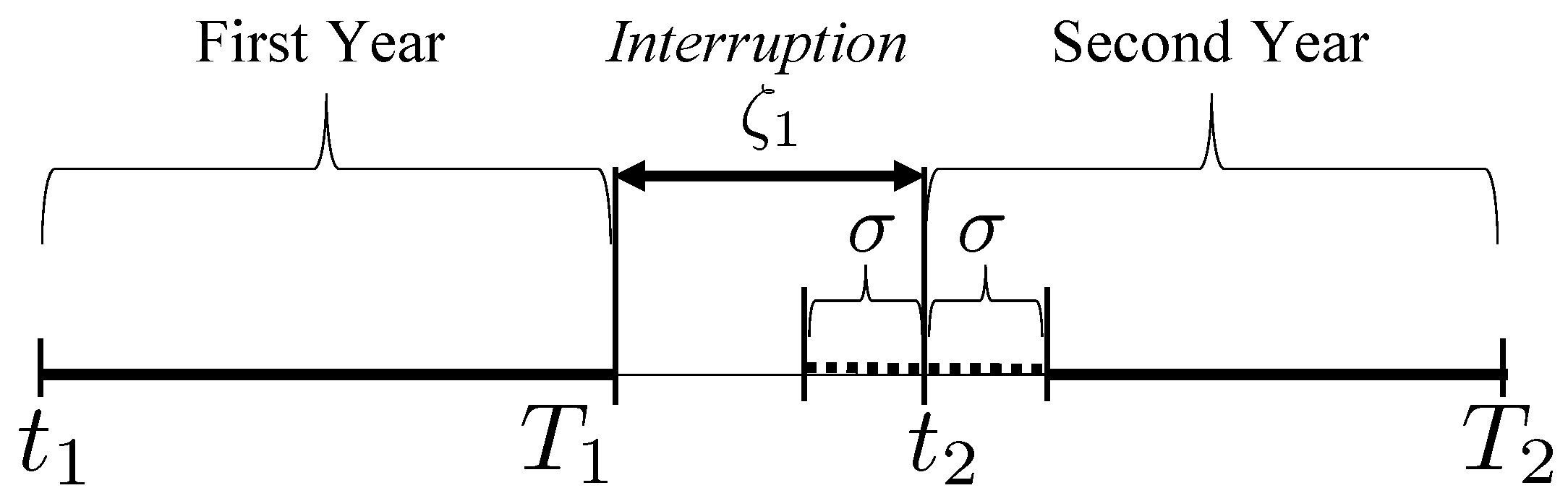
3. Case Study: One-Year and Two-Year Project ()
We consider that the owner considers ordering a one-year or two-year project. First, we examine the optimal decisions of the owner and contractor under the existence of interruption between the first and the second years in a two-year project. Second, we consider those of a one-year project and examine the project selection [preference] of the owner [contractor] by comparing the benefits [profits] of each project. Here, we assume this project begins at and .
3.1. Optimal Decisions under Two-Year Project
When the contractor is required to complete the project within two years (
). Since the optimal solution can be obtained from Equations (
20) and (
21), the optimal amount of work effort at the completion time
can be obtained as
where,
We can see that the amount of work effort is increasing with the increase in the unit reward and the decrease in the unit cost c. We can also observe that the increase in the expected beginning period of the second year decreases . In other words, the increase in the expected length of the interruption decreases the amount of work effort. is a function of the variance of , and satisfies the properties which are shown in the following lemma
Lemma 1. - (i)
increases with the increase in the variance of the length of interruption periods σ, i.e., - (ii)
The value ofhas the lower and upper bound, such as,
It can be said that the total amount of work effort of the two-year project decreases with the increase in the variance of the interruption period from the Lemma 1.
Now, we have the optimal response function of the contractor with respect to
by considering the discussion in the previous section. The optimal reward can be obtained as,
from the condition, Equation (
24). The expected benefit of the owner with the optimal reward can be obtained as,
The first term in Equation (
31) represents the benefit without interruption, which is the benefit of the two-year project can continue without interruption from period 0 to
. The second term is always non-positive, because
and
from Equation (
29) of Lemma 1. It represents that the existence of the interruption periods decreases the owner’s expected benefit. It can be summarized that the properties of the expected benefit for the interruption periods, as the following Proposition 1.
Proposition 1. - (i)
The expected benefit of the owner is decreased by the existence of interruption periods.
- (ii)
The increase in the expected interruption length decreases the expected benefit of the two-year project.
- (iii)
The increase in the variance of the interruption length decreases the expected benefit of the two-year project.
It follows from
and
that Equation (
31) has non-negative value, i.e.,
. Thus, the owner expects positive benefit by selecting two-year project.
As the result of the optimal decision by the owner, the expected amount of work for the two-year project can be obtained as
From this equation, we can observe that the total amount of work is decreased by the existence of interruption because the second term in parentheses becomes negative under the conditions of
and
. It can also be obtained that the expected profit of the contractor under the optimal reward as
The impact of the interruption on the expected profit can be seen in the third and fourth terms of Equation (
33). The third term represents the decrease in the expected profit due to the existence of the interruption period. And the fourth term represents the increase in the expected profit due to the decrease in the fixed cost by suspending the project during the interruption. Thus, the increase or decrease in the expected profit depends on the relative size of the project value
v and the fixed cost
f. Proposition 2 summarizes the properties of the expected profit,
.
Proposition 2. - (i)
The expected profit of the contractor is increased [decreased] by the existence of interruption if the project value v is sufficiently larger [smaller] than the fixed cost f.
- (ii)
The expected profit of the contractor is increased [decreased] with the increase in the expected length of interruption if the project value v is sufficiently larger [smaller] than the fixed cost f.
- (iii)
The expected profit of the contractor is always decreasing with the increase in the variance of interruption length.
In order to implement the two-year project, the expected profit must be greater than or equal to zero. Proposition 2 suggests that projects that are expected to obtain larger profits due to their large project value will be less attractive by becoming interruption length longer or increasing uncertainty.
3.2. Comparison between Projects
Optimal Decision under One-Year Project ()
Suppose that the contractor is required to complete the project by the end of the first year,
. The optimal decision of the contractor is then determined by the following deterministic optimization problem:
subject to
where we assume that
and
. The optimal control can be obtained by following a similar procedure in the two-year project, yielding
This function shows that the optimal amount of work in each week will increase with time t. This is because the cost per unit of work can be discounted by the time discount rate. However, as the completion time becomes longer, the amount of work in each week becomes smaller. This is because the manager can allocate work to more weeks.
As the result of allocating work in each week according to Equation (
36), the project quality achieved at
becomes
The project quality increases as the value of increases. In contrast, increases in the cost of work and the time discount rate reduce the project quality. This is because the benefit of this project is only generated at the completion time , and any increase in the time discount rate lowers the present value of the project. Therefore, an increase in the time discount rate decreases the project quality.
We can derive the optimal amount of work under the optimal reward, by considering the optimal reward which can be derived from Equation (
24) and the optimal amount of work Equation (
37).
And we can also derive the profit of the contractor under the optimal decisions as follows:
The owner’s benefit in the one-year project can be obtained by considering
into the net benefit function defined by Equation (
23).
Equation (
40) represents that the
has non-negative value, i.e.,
, because
and
. Thus, the owner can obtain positive benefit by selecting one-year project. This paper only considers exogenously determined completion time,
and
. The relationship between the completion time and the net benefit function can be obtained as shown in the following lemma,
Lemma 2. There exists an optimal completion time that maximizes,and there also exists an optimal completion time that maximizes, Lemma 2 implies that if the project duration is sufficiently long, it decreases the net benefit by setting the duration longer.
3.3. Project Selection by the Owner
We now discuss the owner’s selection between the one-year and two-year projects. The owner selects one of the projects by following the rule given by Equation (
25). In this case, it can be rewritten as follows,
where,
The following proposition represents the differences in the projects selected by the owner, according to the expected length of the interruption.
Proposition 3. - (i)
The owner selects the two-year project, if the interruption length is sufficiently shorter, i.e.,.
- (ii)
The owner selects ones-year project, if the interruption length is sufficiently longer, i.e.,.
The amount of work effort is also affected by the interruption. Let
denote the difference between those of projects and it is defined as
The following proposition represents the properties of the amount of work effort, according to the selected project.
Proposition 4. - (i)
When the owner selects the two-year project, the amount of work effort of the two-year project is always larger than that of the one-year project.
- (ii)
When the owner selects the one-year project,
- (a)
the amount of work effort of the one-year project is larger than that of the two-year project, if the interruption period is longer than, i.e.,.
- (b)
the amount of work effort of the one-year project is smaller than that of the two-year project, if the interruption period is shorter than, i.e.,.
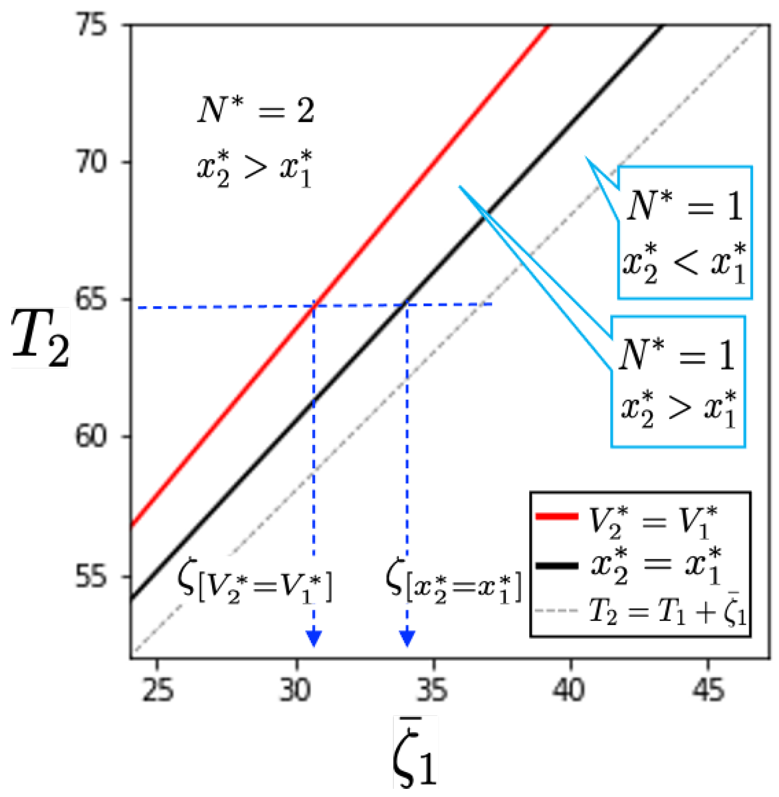
where,and.
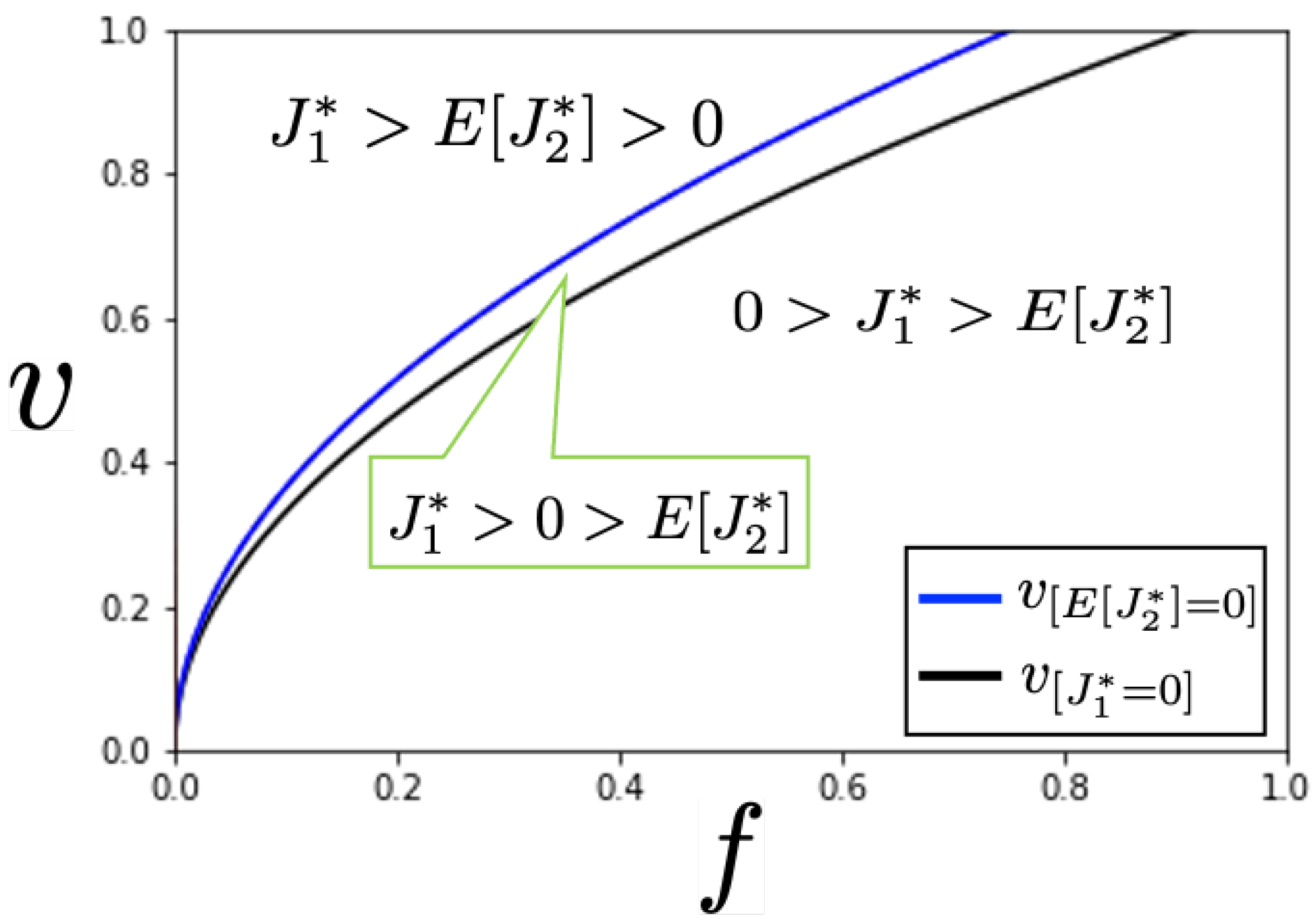
Figure 2 summarizes the Propositions 3 and 4 in the deterministic case (
).
must be larger than
for consistency, only upper-left side of the
Figure 2 can be considered. Since
, the threshold value
is always located on the left-hand side of
. Thus, when the interruption length
is shorter than
, the owner selects the two-year project and the resulted amount of work effort is larger than that of the one-year project. On the other hand, if
holds, even though the amount of work effort is larger for the one-year project, the two-year project is ordered. Furthermore, the longer the interruption length, the less duration is available for the two-year project, so the one-year project is selected, and the resulted amount of work effort is larger than that of the two-year project.
The threshold values defined in Equations (
45) and (
47) are affected by the variance of interruption length
. The following proposition can be derived and it implies that the conditions under which the two-year project is selected vary with uncertainty in the interruption.
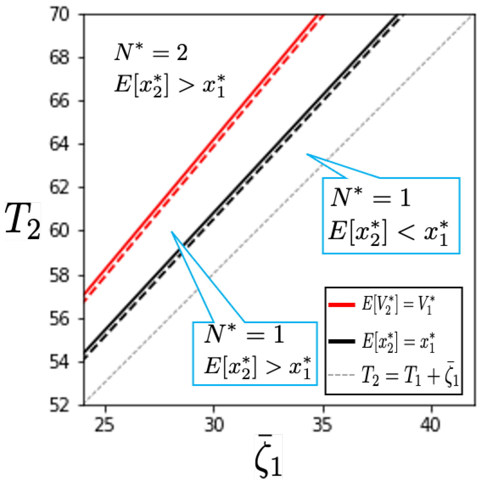
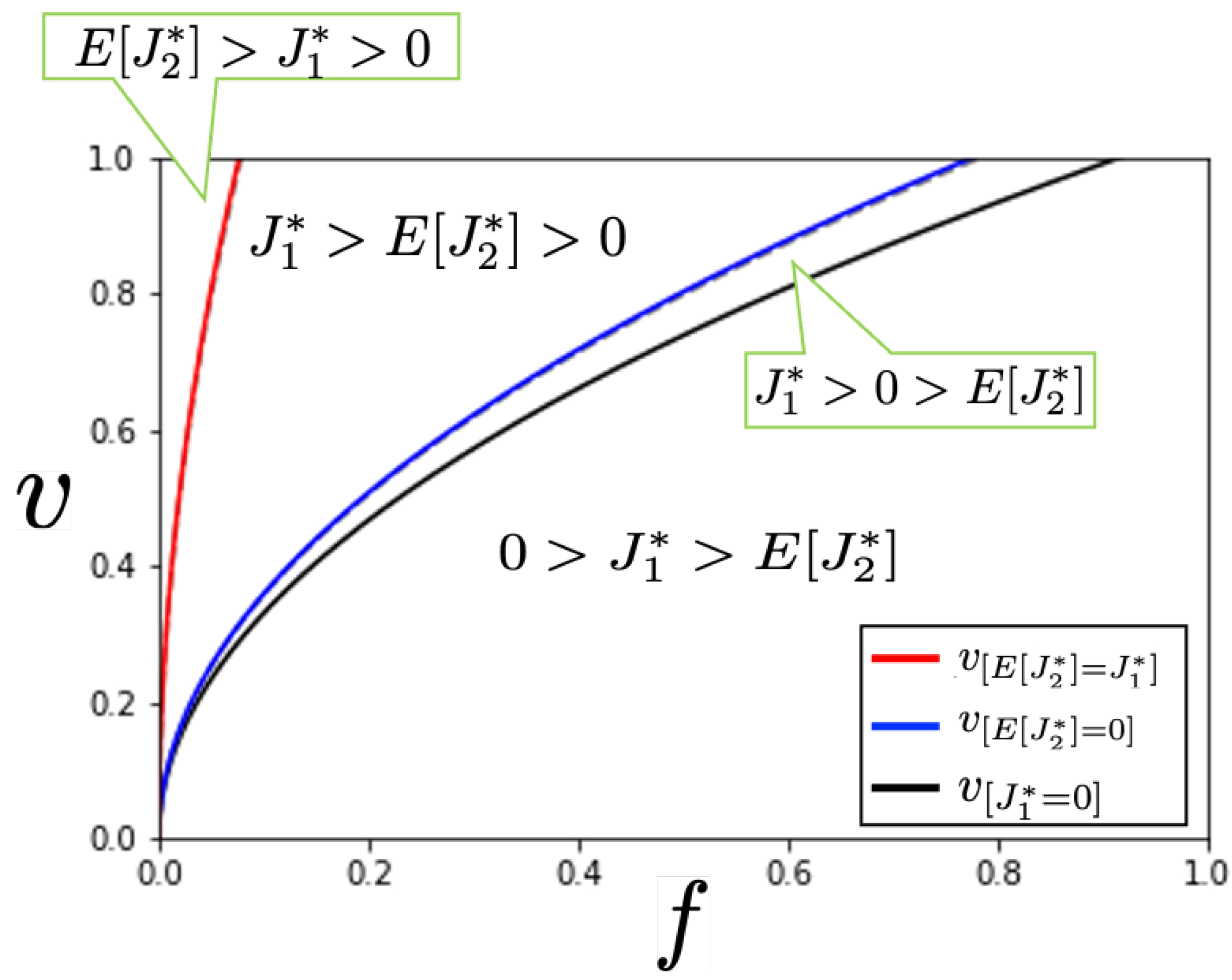
Proposition 5. As the variance of the interruption length increases, the threshold value of selecting the two-year project becomes smaller, i.e.,. And the threshold value of characterizing the relative size of the projects also decreases with the increase in the variance, i.e.,.
Proposition 5 represents that the allowable interruption length to select the two-year project becomes smaller with the increase in the variance of interruption length. It suggests that long-term projects might be more difficult to be ordered under conditions where global warming increases uncertainty in the interruption.
Figure 3 is a graphical representation of Proposition 5, which represents the impact of interruption on
and
. (See
Appendix A for the numerical setting.) The dotted lines in
Figure 3 show the
and
under the deterministic case, which are shown in
Figure 2. We can see that these threshold values are shifted to the left-hand side. This suggests that as the uncertainty of the interruption period increases, the owner will order a two-year project when the interruption period is shorter.
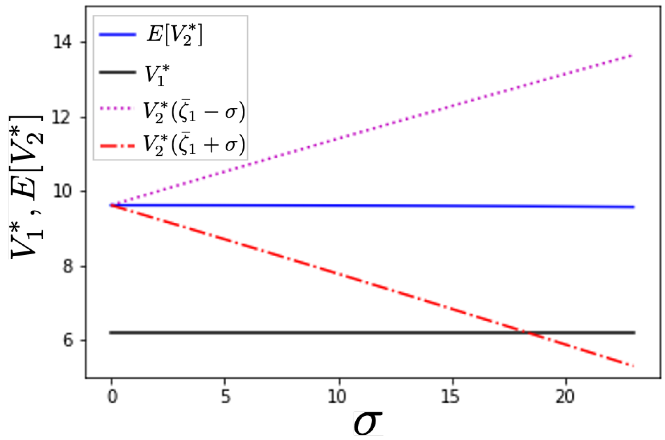
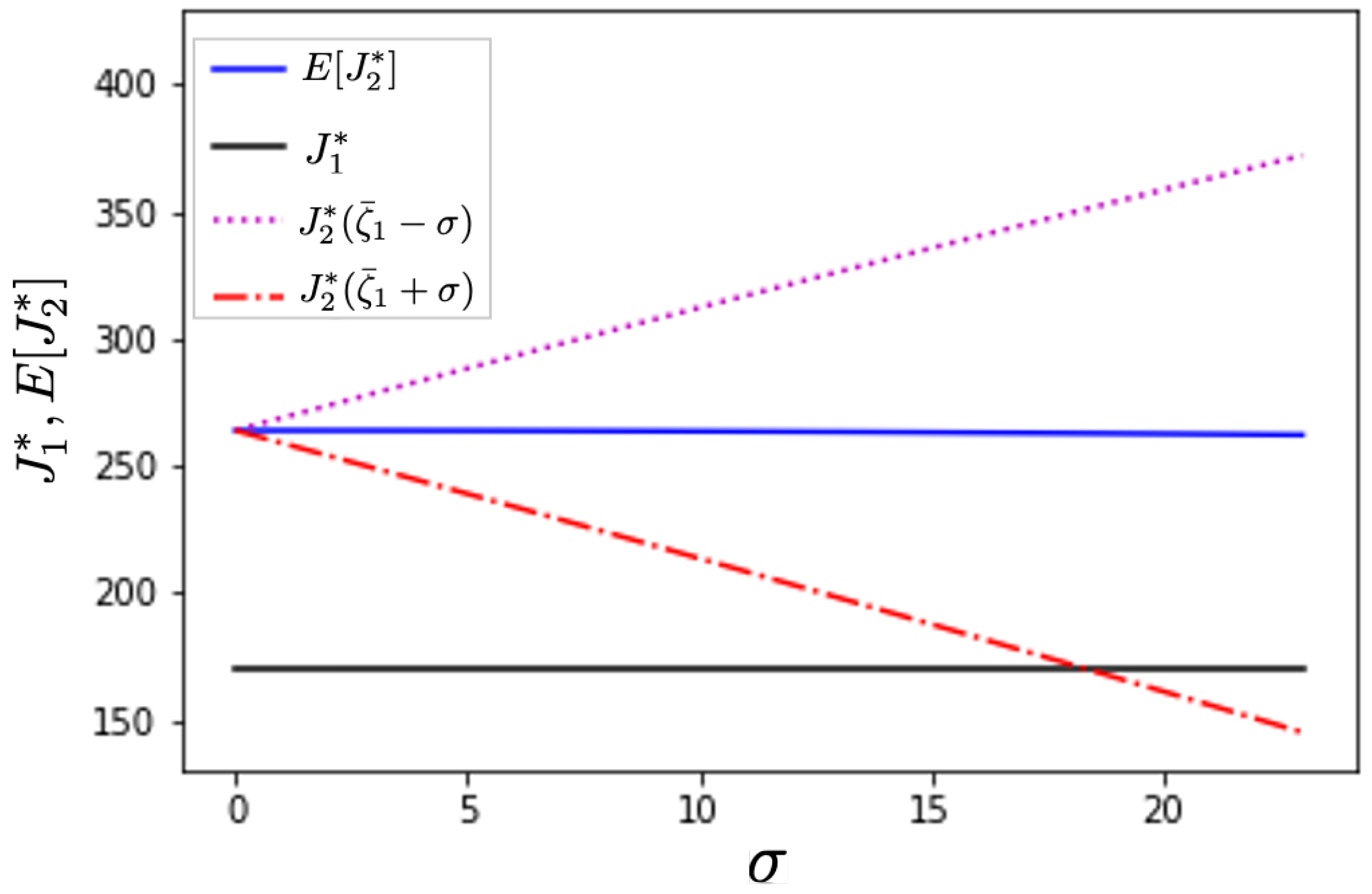
As the uncertainty in interruption periods changes, the owner’s benefit also changes. The variance of the owner’s benefit can be defined as
Figure 4 shows the relationship between
and the benefits. This figure shows the case that the two-year project is selected by the owner because the expected benefit of the two-year project is larger than that of the one-year project, i.e.,
. We can see that the changes in
is smaller than changes in
and
, which show the resulting benefits after the interruption.
represents the possible shortest interruption periods in the uniform distribution
. Under the shortest interruption case, the owner can obtain the largest benefit and it increases with the variance
. On the other hand,
gives the longest interruption periods, it results the smallest benefit after
.
decreases with the increase in
. And it is found that
becomes lower than
in the case of large
. In the symmetric uniform distribution considered here, the increase in uncertainty causes a small change in the expected benefit, but a large change in the resulting benefit might be smaller than that of the one-year project, even though the two-year project was selected because of its larger expected benefit.
3.4. Project Preference of the Contractor
In this section, we compare the expected profits of the contractor obtained from each of the projects, to analyze the impact of the interruption on the contractor. We assume that the contractor prefers the project that can achieve a larger expected profit. The contractor’s preference under the owner’s order can be summarized as the following proposition.
Proposition 6. - (i)
When the owner orders the one-year project and the project is implemented, the contractor preferred the one-year project than the two-year project, i.e.,.
- (ii)
When the owner orders the two-year project and the project is implemented, the contractor preferred the two-year [one-year] project, if the project value v is sufficiently larger [smaller] than the fixed cost f.
Proposition 6 (i) can be graphically represented as
Figure 5. It represents the stochastic interruption with
(weeks). First, the condition of implementing the one-year project is given by the area on the upper side of
. The contractor prefers the one-year project, regardless of its project value
v, under the condition of
. Therefore, if the one-year project is implemented, the contractor prefers the one-year project.
Proposition 6 (ii) can be graphically represented in
Figure 6. First, the condition of implementing the two-year project is given by the area on the upper-left side of
(blue line). The contractor prefers the two-year project, if its project value
v is larger than
. If the project value
v lies between
and
, the two-year project will be ordered by the owner, even though the one-year project would be more preferable by the contractor. The grey dotted line shows the value of
in the deterministic case (
(weeks)), we can see that
is increased by considering the variation of interruption length. It suggests that a larger project value is needed for the two-year project to be preferred by the contractor in the presence of uncertainty.
As the interruption length changes, the contractor’s profit also changes. The variance of the contractor’s profit can be given by
Figure 7 shows the changes in the contractor’s expected profit
and resulting profits
,
,
under the various value of
.
Figure 7 is the case that the contractor prefers the two-year project, because
. As the increase in
, the smallest profit which is obtained in the longest interruption, i.e., in the case of
, becomes smaller than
. Therefore, as we have discussed the owner’s benefit, it is suggested that the resulting profit of the two-year project may be lower than that of the one-year project, even though the two-year project was preferred by the contractor in terms of the expected profit. However, the preferred project by the contractor can be consistent with the selected project by decreasing the fixed costs
f relative to the benefit
v. As shown in
Figure 7, decreasing the fixed costs decreases the difference of the contractor’s profits between one-year and two-year projects and it can finally achieve a situation where the contractor prefers a two-year project(
).


