
A New Methodology for Reference Evapotranspiration Prediction and Uncertainty Analysis under Climate Change Conditions Based on Machine Learning, Multi Criteria Decision Making and Monte Carlo Methods


Abstract
:1. Introduction
2. Materials and Methods
2.1. Present Work Steps
- Adequate and reliable data is required.
- Machine learning requires preprocessing of input data to achieve accurate results.
- The Monte Carlo method requires probabilistic distribution functions to generate input data.
- ETo data are estimated by FAO-56 PM method based on meteorological data (minimum T (min-T), maximum T (max-T), solar radiation, humidity, wind speed and sunny hours) at the different stations.
- The data is divided into training (70%) and testing (30%) periods.
- Six machine learning algorithms, including MLR, MNLR, MARS, M5, RF and LSBoost are employed for estimating CIP removal value.
- Because in modeling ETo and comparing algorithms, various factors such as evaluation criteria and calculation time affect selecting the best model, the TOPSIS method is used to select the best algorithm. This process is as follows:
- Evaluation criteria, including MAE, RMSE, R, MARE, RRMSE and the run times of algorithms, are considered as criteria of the TOPSIS method.
- Algorithms including MLR, MNLR, MARS, M5, RF and LSBoost are considered as alternatives.
- The TOPSIS method is used under seven scenarios to select the best algorithm. The lambda time weight varies from 0.091 to 0, and the lambda weight of the other criteria is the same in all scenarios.
- In the last step in each scenario, the algorithm with the highest score is selected as the best algorithm. Figure A1 (Appendix A.1) shows the TOPSIS structure for selecting the best algorithm.
- At this step, the delta CF method is used to downscale T and P using three models (ACCESS-ESM1-5, CanESM5 and MRI-ESM2-0) and three scenarios (SCF, SCM and SCS) were used.
- ETo prediction for the period 2021–2050 under the influence of climate change is performed by downscaled T and P data and the best algorithm in nine stations.
- Uncertainty analysis of models and scenarios is performed using the MCM in different stations.
2.2. Penman-Monteith Equation (FAO-56 PM)
2.3. Multiple Linear Regression (MLR)
2.4. Multiple Non-Linear Regression (MNLR)
2.5. Multivariate Adaptive Regression Splines (MARS)
2.6. M5 Model Tree (M5)
- Dividing the inputs area into several subsets and using a linear regression model according to partial attribute values for each subset.
- In each node, a linear regression is established.
2.7. Random Forest (RF)
2.8. Least-Squares Boost (LSBoost)
2.9. Technique for Order of Preference by Similarity to Ideal Solution (TOPSIS)
2.10. Delta Change Factor (CF) Method for Downscaling CMIP6 GCMs Data
2.11. Monte Carlo Method (MCM)
- Each input data is assigned an appropriate distribution function.
- Using the selected distribution functions, 1000 new data time series are generated for each input.
- The output corresponding to each data time series generated by the distribution functions is predicted.
- Predicting new outputs, a 95% prediction confidence interval is obtained using the values generated for each observation to quantify the prediction uncertainties.
- Sort upper and lower band of 95% confidence interval for each time series.
- The upper quartile (97.5%) and the lower quartile (2.5%) of the 95% band are determined.
- The R-factor coefficient is calculated using the following formula. The lower the value of this coefficient, the less uncertainty.
2.12. Evaluation of Model Performance
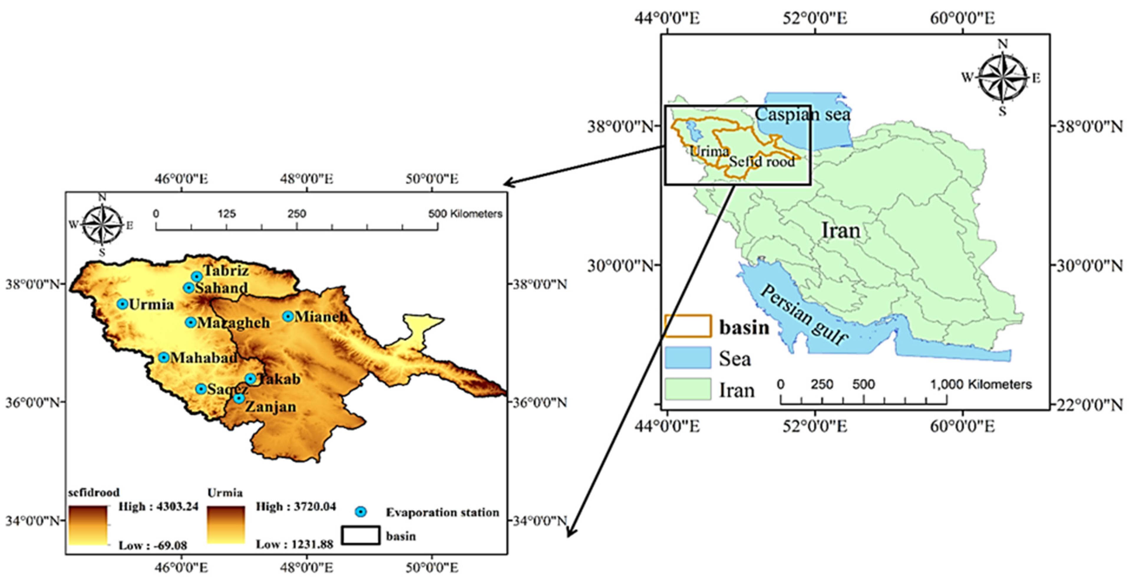
2.13. Study Area and Data Materials
2.14. GCMs and Future Climate Change Scenarios
3. Results and Discussion
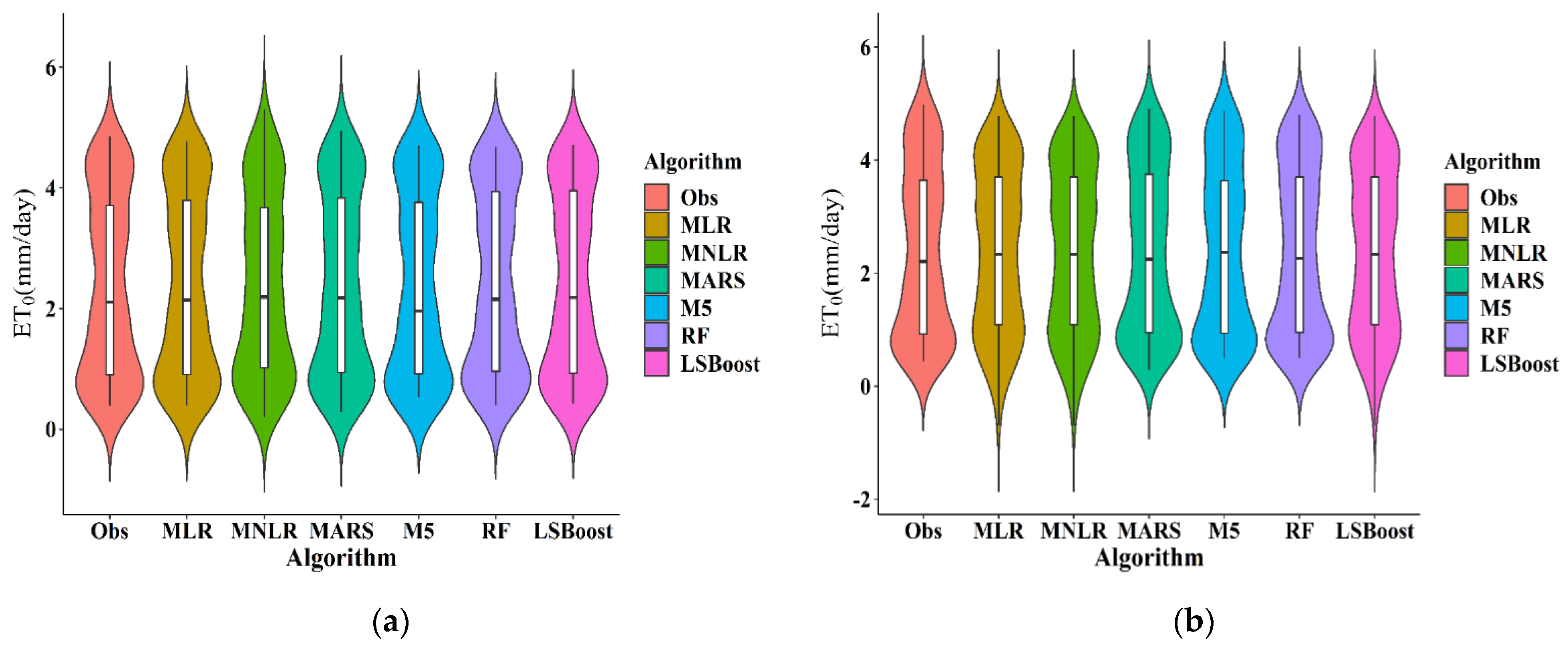
3.1. ETo Modeling by Machine Learning
3.2. Selecting the Best Machine Learning
3.3. Downscaling T and P
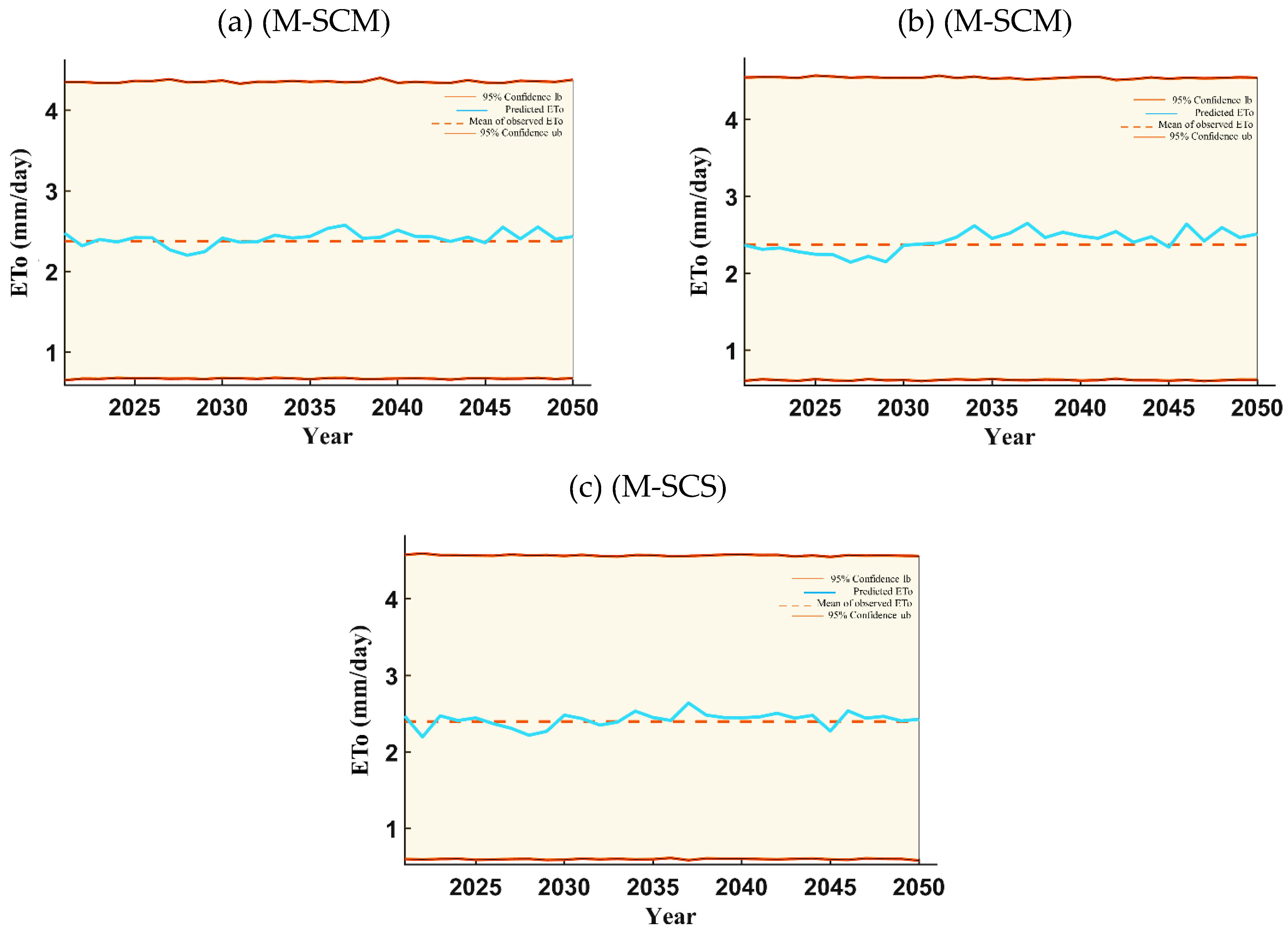
3.4. Prediction of ETo
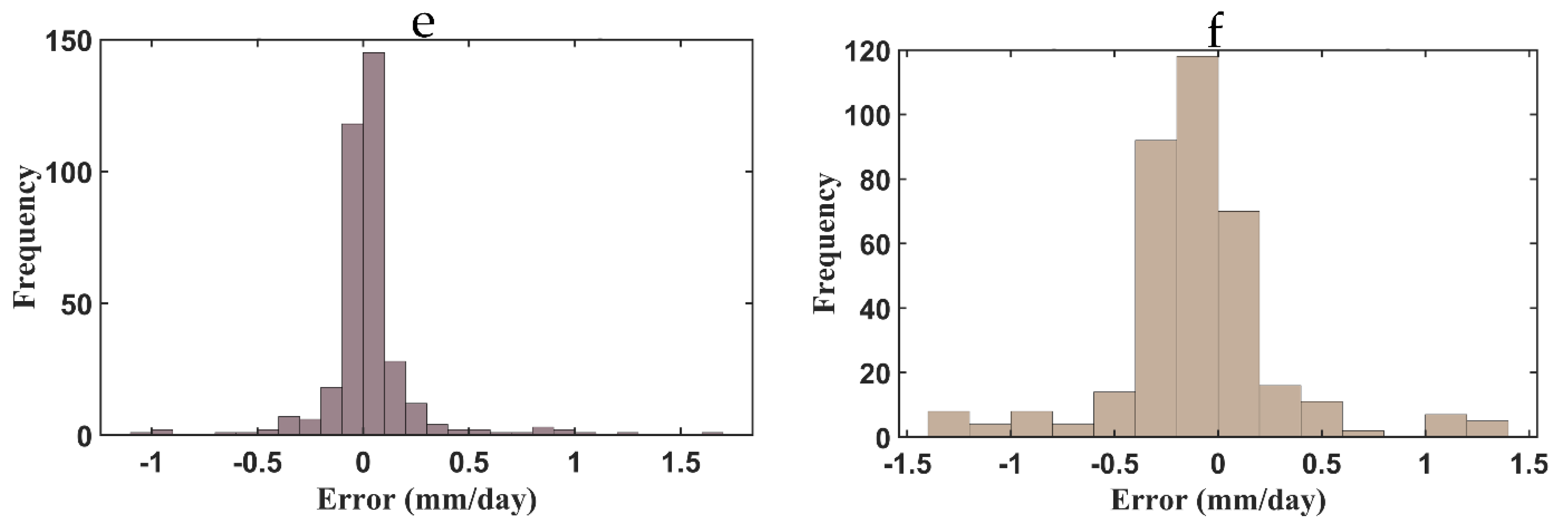
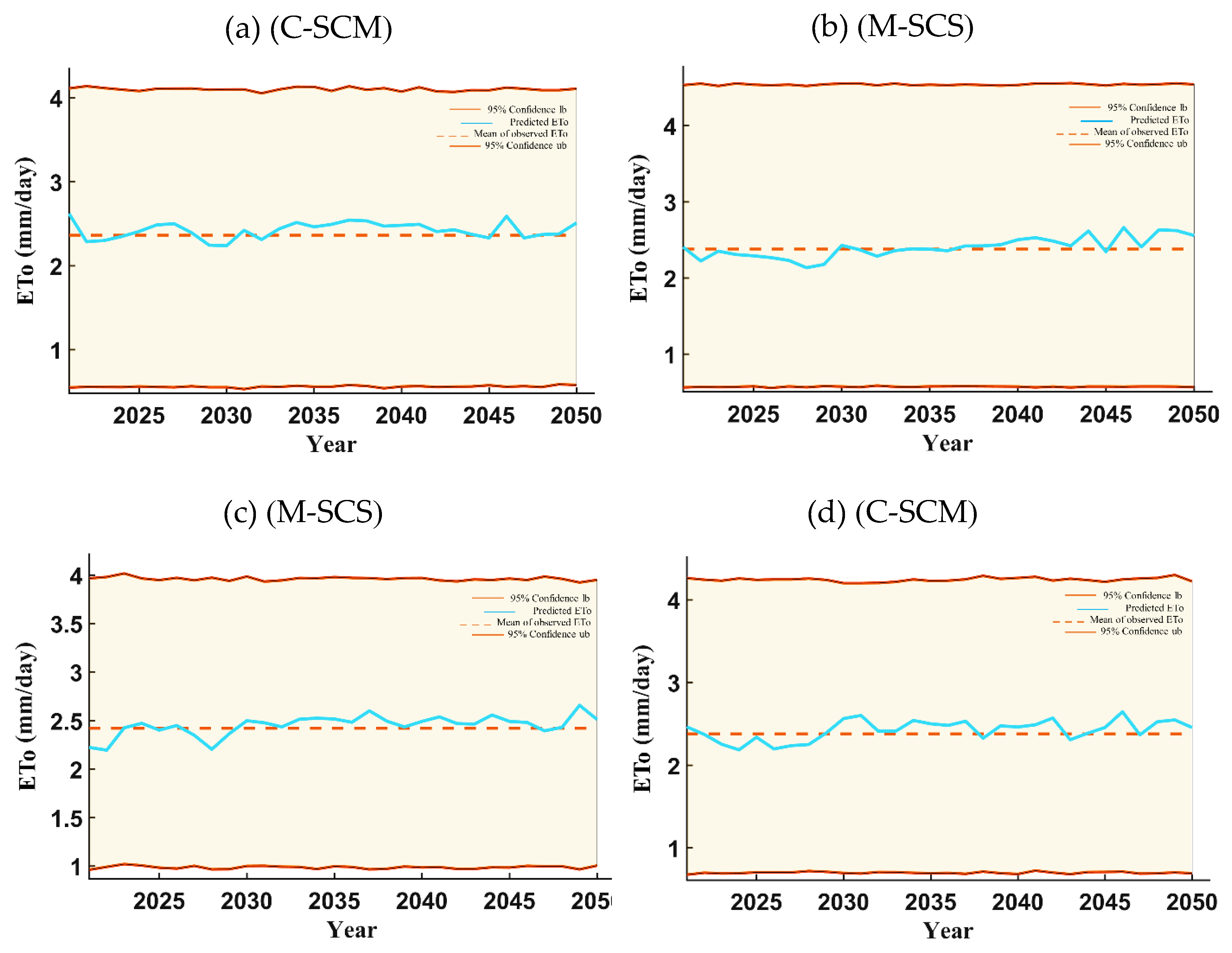
3.5. Uncertainty Analysis
4. Conclusions
- The accuracy of machine learning algorithms for ETo modeling was very good. However, TOPSIS results showed that LSBoost (score = 0.96) was the best algorithm. The average evaluation criteria obtained by LSBoost in the nine stations were in a very good range (MAE = 0.18, RMSE = 0.06, R = 0.99, MARE = 0.11, RRMSE = 0.04, Time = 1.11 s).
- Downscaling results showed that future monthly changes of mean T and P at all stations and scenarios increased. The highest increase in T was related to the Zanjan station in the CanESM5 model and SCF scenario (0.83 °C). In addition, the highest increase of P (11.20 mm/day) was related to the Mianeh station in the CanESM5 model and SCS scenario.
- The mean amount of ETo in all stations increased in all models and scenarios. The highest increase was related to the Urmia station (3.84%), and the lowest was the Mahabad station (0.50%).
- The GCMs and scenarios of CMIP6 had high uncertainty. However, for considered GCMs and scenarios, the lowest and highest uncertainty in the MRI-ESM2-0 model and SCS scenario were in the Mianeh (R-factor = 1.979) and Mahabad (R-factor = 2.824) stations, respectively.
Author Contributions
Funding
Institutional Review Board Statement
Informed Consent Statement
Data Availability Statement
Conflicts of Interest
Appendix A
Appendix A.1

Appendix A.2
Appendix A.3

Appendix A.4

Appendix A.5
Appendix A.6

Appendix A.7
Appendix A.8

| Station | Basin | Parameter | Min T (°C) | Mean T (°C) | Max T (°C) | Humidity (%) | Wind Speed (m/s) | P (mm/Month) | ETo (mm/Day) |
|---|---|---|---|---|---|---|---|---|---|
| Tabriz | Urmia | Std | 7.78 | 12.84 | 18.84 | 51.23 | 3.12 | 20.89 | 7.81 |
| Mean | 8.72 | 9.94 | 10.76 | 14.25 | 1.01 | 19.58 | 2.37 | ||
| Sahand | Urmia | Std | 7.40 | 12.00 | 16.96 | 49.74 | 3.73 | 19.16 | 8.06 |
| Mean | 8.08 | 9.37 | 10.19 | 13.23 | 1.92 | 18.50 | 2.36 | ||
| Urmia | Urmia | Std | 5.36 | 11.33 | 17.94 | 58.93 | 1.86 | 26.28 | 8.13 |
| Mean | 7.44 | 9.13 | 9.86 | 11.24 | 0.86 | 28.07 | 2.37 | ||
| Maragheh | Urmia | Std | 8.14 | 12.87 | 18.90 | 49.32 | 2.72 | 25.13 | 8.10 |
| Mean | 8.15 | 9.66 | 10.49 | 14.86 | 1.29 | 26.84 | 2.38 | ||
| Mianeh | Sefidrood | Std | 7.69 | 14.04 | 20.62 | 51.71 | 1.80 | 23.49 | 7.97 |
| Mean | 7.96 | 10.59 | 10.97 | 14.61 | 0.97 | 22.13 | 2.42 | ||
| Mahabad | Urmia | Std | 7.18 | 13.06 | 19.41 | 52.29 | 2.08 | 33.59 | 8.03 |
| Mean | 7.10 | 9.33 | 10.35 | 14.94 | 0.87 | 34.65 | 2.40 | ||
| Saqez | Urmia | Std | 3.03 | 11.36 | 18.94 | 53.75 | 2.16 | 38.37 | 8.20 |
| Mean | 7.08 | 9.71 | 10.96 | 17.36 | 0.95 | 40.96 | 2.38 | ||
| Takab | Urmia | Std | 2.53 | 10.12 | 16.48 | 54.24 | 2.13 | 25.87 | 8.00 |
| Mean | 7.38 | 9.80 | 10.80 | 16.72 | 0.90 | 24.26 | 2.33 | ||
| Zanjan | Sefidrood | Std | 2.13 | 8.71 | 14.89 | 53.93 | 3.59 | 32.02 | 8.38 |
| Mean | 7.33 | 9.19 | 10.09 | 16.73 | 1.15 | 31.15 | 2.32 |
Appendix A.9
Appendix A.9.1. Fossil-Fueled Recovery
Appendix A.9.2. Moderate Green Stimulus
Appendix A.9.3. Strong Green Stimulus
Appendix B
Appendix B.1
| Train | Test | |||||||||
|---|---|---|---|---|---|---|---|---|---|---|
| Sahand | ||||||||||
| MAE | RMSE | R | MARE | RRMSE | MAE | RMSE | R | MARE | RRMSE | |
| MLR | 0.40 | 0.27 | 0.93 | 0.32 | 0.18 | 0.28 | 0.13 | 0.97 | 0.24 | 0.08 |
| MNLR | 0.33 | 0.21 | 0.95 | 0.23 | 0.14 | 0.25 | 0.09 | 0.98 | 0.17 | 0.06 |
| MARS | 0.33 | 0.22 | 0.95 | 0.22 | 0.15 | 0.24 | 0.08 | 0.98 | 0.15 | 0.06 |
| M5 | 0.22 | 0.16 | 0.96 | 0.16 | 0.11 | 0.23 | 0.16 | 0.97 | 0.17 | 0.10 |
| RF | 0.21 | 0.14 | 0.97 | 0.15 | 0.10 | 0.19 | 0.06 | 0.99 | 0.13 | 0.04 |
| LSBoost | 0.15 | 0.13 | 0.97 | 0.12 | 0.09 | 0.20 | 0.07 | 0.98 | 0.14 | 0.05 |
| Maragheh | ||||||||||
| MLR | 0.25 | 0.10 | 0.97 | 0.17 | 0.07 | 0.56 | 1.11 | 0.78 | 0.35 | 0.73 |
| MNLR | 0.19 | 0.07 | 0.98 | 0.12 | 0.05 | 0.50 | 1.06 | 0.79 | 0.27 | 0.69 |
| MARS | 0.23 | 0.08 | 0.98 | 0.14 | 0.06 | 0.23 | 0.07 | 0.99 | 0.16 | 0.05 |
| M5 | 0.10 | 0.02 | 0.99 | 0.05 | 0.02 | 0.20 | 0.07 | 0.98 | 0.12 | 0.05 |
| RF | 0.13 | 0.03 | 0.99 | 0.07 | 0.02 | 0.22 | 0.08 | 0.99 | 0.15 | 0.05 |
| LSBoost | 0.02 | 0.00 | 1.00 | 0.01 | 0.00 | 0.19 | 0.06 | 0.99 | 0.13 | 0.04 |
| Mianeh | ||||||||||
| MLR | 0.32 | 0.20 | 0.95 | 0.27 | 0.13 | 0.56 | 1.14 | 0.79 | 0.36 | 0.74 |
| MNLR | 0.24 | 0.13 | 0.97 | 0.17 | 0.09 | 0.46 | 1.07 | 0.81 | 0.23 | 0.69 |
| MARS | 0.23 | 0.13 | 0.97 | 0.15 | 0.08 | 0.17 | 0.05 | 0.99 | 0.10 | 0.03 |
| M5 | 0.12 | 0.09 | 0.98 | 0.08 | 0.06 | 0.15 | 0.05 | 0.99 | 0.10 | 0.03 |
| RF | 0.16 | 0.11 | 0.98 | 0.12 | 0.07 | 0.15 | 0.04 | 0.99 | 0.09 | 0.02 |
| LSBoost | 0.13 | 0.09 | 0.98 | 0.10 | 0.06 | 0.14 | 0.03 | 0.99 | 0.09 | 0.02 |
| Saqez | ||||||||||
| MLR | 0.30 | 0.14 | 0.99 | 0.23 | 0.10 | 0.31 | 0.15 | 0.97 | 0.26 | 0.10 |
| MNLR | 0.23 | 0.08 | 0.98 | 0.15 | 0.06 | 0.24 | 0.08 | 0.98 | 0.18 | 0.06 |
| MARS | 0.18 | 0.05 | 0.99 | 0.11 | 0.04 | 0.20 | 0.06 | 0.98 | 0.14 | 0.04 |
| M5 | 0.12 | 0.03 | 0.99 | 0.07 | 0.02 | 0.16 | 0.09 | 0.98 | 0.09 | 0.06 |
| RF | 0.11 | 0.02 | 0.99 | 0.07 | 0.02 | 0.17 | 0.05 | 0.99 | 0.12 | 0.03 |
| LSBoost | 0.02 | 0.00 | 1.00 | 0.02 | 0.00 | 0.15 | 0.04 | 0.99 | 0.11 | 0.03 |
| Takab | ||||||||||
| MLR | 0.28 | 0.14 | 0.96 | 0.21 | 0.10 | 0.26 | 0.09 | 0.98 | 0.20 | 0.07 |
| MNLR | 0.24 | 0.11 | 0.97 | 0.16 | 0.08 | 0.22 | 0.06 | 0.98 | 0.15 | 0.05 |
| MARS | 0.19 | 0.08 | 0.98 | 0.12 | 0.06 | 0.19 | 0.05 | 0.99 | 0.11 | 0.04 |
| M5 | 0.13 | 0.06 | 0.98 | 0.08 | 0.04 | 0.22 | 0.13 | 0.97 | 0.13 | 0.09 |
| RF | 0.13 | 0.06 | 0.99 | 0.08 | 0.04 | 0.20 | 0.07 | 0.98 | 0.12 | 0.05 |
| LSBoost | 0.07 | 0.04 | 0.99 | 0.05 | 0.03 | 0.21 | 0.09 | 0.98 | 0.13 | 0.06 |
| Zanjan | ||||||||||
| MLR | 0.39 | 0.27 | 0.92 | 0.28 | 0.20 | 0.29 | 0.12 | 0.97 | 0.22 | 0.08 |
| MNLR | 0.34 | 0.24 | 0.93 | 0.22 | 0.18 | 0.22 | 0.07 | 0.98 | 0.14 | 0.05 |
| MARS | 0.31 | 0.22 | 0.94 | 0.21 | 0.16 | 0.22 | 0.07 | 0.99 | 0.14 | 0.05 |
| M5 | 0.27 | 0.21 | 0.94 | 0.17 | 0.15 | 0.20 | 0.10 | 0.98 | 0.12 | 0.07 |
| RF | 0.25 | 0.19 | 0.94 | 0.16 | 0.15 | 0.16 | 0.05 | 0.99 | 0.11 | 0.03 |
| LSBoost | 0.31 | 0.22 | 0.94 | 0.18 | 0.16 | 0.20 | 0.07 | 0.98 | 0.12 | 0.05 |
Appendix B.2

Appendix B.3


Appendix B.4


Appendix B.5
| Station | Model-Scenario | ΔT (°C) | ΔP (mm/Day) | Station | Model-Scenario | ΔT (°C) | ΔP (mm/Day) |
|---|---|---|---|---|---|---|---|
| Sahand | A-SCF | 0.53 | 2.35 | Saqez | A-SCF | 0.51 | 3.56 |
| A-SCM | 0.34 | 1.84 | A-SCM | 0.32 | 3.23 | ||
| A-SCS | 0.45 | 1.46 | A-SCS | 0.43 | 3.30 | ||
| C-SCF | 0.69 | 2.37 | C-SCF | 0.71 | 3.95 | ||
| C-SCM | 0.55 | 2.26 | C-SCM | 0.54 | 4.57 | ||
| C-SCS | 0.53 | 2.29 | C-SCS | 0.52 | 2.46 | ||
| M-SCF | 0.61 | −0.09 | M-SCF | 0.60 | −0.98 | ||
| M-SCM | 0.45 | 1.43 | M-SCM | 0.44 | 3.10 | ||
| M-SCS | 0.42 | −0.01 | M-SCS | 0.41 | −1.43 | ||
| Maragheh | A-SCF | 0.53 | 2.05 | Takab | A-SCF | 0.51 | 2.95 |
| A-SCM | 0.34 | 1.61 | A-SCM | 0.32 | 2.78 | ||
| A-SCS | 0.45 | 1.43 | A-SCS | 0.43 | 2.74 | ||
| C-SCF | 0.69 | 2.31 | C-SCF | 0.78 | 6.70 | ||
| C-SCM | 0.55 | 2.70 | C-SCM | 0.71 | 7.98 | ||
| C-SCS | 0.53 | 2.66 | C-SCS | 0.63 | 10.94 | ||
| M-SCF | 0.61 | −0.30 | M-SCF | 0.63 | −0.59 | ||
| M-SCM | 0.45 | 1.63 | M-SCM | 0.47 | 1.29 | ||
| M-SCS | 0.42 | −0.65 | M-SCS | 0.45 | −0.35 | ||
| Mianeh | A-SCF | 0.53 | 2.58 | Zanjan | A-SCF | 0.51 | 3.21 |
| A-SCM | 0.34 | 2.47 | A-SCM | 0.32 | 3.20 | ||
| A-SCS | 0.45 | 2.19 | A-SCS | 0.43 | 3.33 | ||
| C-SCF | 0.78 | 6.65 | C-SCF | 0.83 | 6.01 | ||
| C-SCM | 0.71 | 7.03 | C-SCM | 0.71 | 7.27 | ||
| C-SCS | 0.63 | 11.20 | C-SCS | 0.62 | 7.58 | ||
| M-SCF | 0.64 | 0.66 | M-SCF | 0.63 | −0.76 | ||
| M-SCM | 0.49 | 2.23 | M-SCM | 0.47 | 1.42 | ||
| M-SCS | 0.46 | −0.09 | M-SCS | 0.45 | −0.77 |
Appendix B.6

Appendix B.7
| A-SCF | A-SCM | A-SCS | C-SCF | C-SCM | C-SCS | M-SCF | M-SCM | M-SCS | |
|---|---|---|---|---|---|---|---|---|---|
| Sahand | |||||||||
| Mean-Obs | 2.36 | 2.36 | 2.36 | 2.36 | 2.36 | 2.36 | 2.36 | 2.36 | 2.36 |
| Mean-Pred | 2.44 | 2.41 | 2.43 | 2.44 | 2.42 | 2.42 | 2.41 | 2.41 | 2.41 |
| Min-Obs | 0.43 | 0.43 | 0.43 | 0.43 | 0.43 | 0.43 | 0.43 | 0.43 | 0.43 |
| Min-Pred | 0.39 | 0.37 | 0.35 | 0.36 | 0.32 | 0.38 | 0.36 | 0.36 | 0.36 |
| Max-Obs | 4.86 | 4.86 | 4.86 | 4.86 | 4.86 | 4.86 | 4.86 | 4.86 | 4.86 |
| Max-Pred | 4.83 | 4.80 | 4.78 | 4.86 | 4.83 | 4.82 | 4.80 | 4.81 | 4.79 |
| Change mean (%) | 3.28 | 1.83 | 2.69 | 3.03 | 2.55 | 2.31 | 2.08 | 1.84 | 2.09 |
| Maragheh | |||||||||
| Mean-Obs | 2.38 | 2.38 | 2.38 | 2.38 | 2.38 | 2.38 | 2.38 | 2.38 | 2.38 |
| Mean-Pred | 2.43 | 2.41 | 2.43 | 2.41 | 2.40 | 2.41 | 2.42 | 2.40 | 2.40 |
| Min-Obs | 0.48 | 0.48 | 0.48 | 0.48 | 0.48 | 0.48 | 0.48 | 0.48 | 0.48 |
| Min-Pred | 0.47 | 0.45 | 0.47 | 0.48 | 0.45 | 0.42 | 0.47 | 0.46 | 0.46 |
| Max-Obs | 4.93 | 4.93 | 4.93 | 4.93 | 4.93 | 4.93 | 4.93 | 4.93 | 4.93 |
| Max-Pred | 4.92 | 4.89 | 4.90 | 4.87 | 4.97 | 4.95 | 4.90 | 4.86 | 4.93 |
| Change mean (%) | 2.28 | 1.30 | 1.96 | 1.33 | 0.84 | 1.20 | 1.57 | 0.98 | 0.87 |
| Mianeh | |||||||||
| Mean-Obs | 2.42 | 2.42 | 2.42 | 2.42 | 2.42 | 2.42 | 2.42 | 2.42 | 2.42 |
| Mean-Pred | 2.47 | 2.44 | 2.46 | 2.48 | 2.46 | 2.46 | 2.47 | 2.45 | 2.45 |
| Min-Obs | 0.39 | 0.39 | 0.39 | 0.39 | 0.39 | 0.39 | 0.39 | 0.39 | 0.39 |
| Min-Pred | 0.38 | 0.39 | 0.41 | 0.45 | 0.40 | 0.39 | 0.39 | 0.46 | 0.37 |
| Max-Obs | 5.09 | 5.09 | 5.09 | 5.09 | 5.09 | 5.09 | 5.09 | 5.09 | 5.09 |
| Max-Pred | 4.84 | 4.87 | 4.89 | 4.88 | 4.82 | 4.81 | 4.83 | 4.84 | 4.84 |
| Change mean (%) | 1.93 | 0.68 | 1.36 | 2.20 | 1.77 | 1.70 | 1.85 | 1.11 | 1.29 |
| Saqez | |||||||||
| Mean-Obs | 2.38 | 2.38 | 2.38 | 2.38 | 2.38 | 2.38 | 2.38 | 2.38 | 2.38 |
| Mean-Pred | 2.43 | 2.40 | 2.44 | 2.44 | 2.43 | 2.43 | 2.45 | 2.43 | 2.42 |
| Min-Obs | 0.45 | 0.45 | 0.45 | 0.45 | 0.45 | 0.45 | 0.45 | 0.45 | 0.45 |
| Min-Pred | 0.46 | 0.46 | 0.46 | 0.46 | 0.36 | 0.42 | 0.44 | 0.43 | 0.46 |
| Max-Obs | 4.91 | 4.91 | 4.91 | 4.91 | 4.91 | 4.91 | 4.91 | 4.91 | 4.91 |
| Max-Pred | 4.87 | 4.86 | 4.86 | 4.87 | 4.92 | 4.84 | 4.93 | 4.88 | 4.93 |
| Change mean (%) | 2.06 | 0.87 | 2.38 | 2.65 | 1.91 | 2.16 | 2.80 | 1.98 | 1.69 |
| Takab | |||||||||
| Mean-Obs | 2.33 | 2.33 | 2.33 | 2.33 | 2.33 | 2.33 | 2.33 | 2.33 | 2.33 |
| Mean-Pred | 2.38 | 2.35 | 2.38 | 2.39 | 2.39 | 2.38 | 2.38 | 2.37 | 2.37 |
| Min-Obs | 0.47 | 0.47 | 0.47 | 0.47 | 0.47 | 0.47 | 0.47 | 0.47 | 0.47 |
| Min-Pred | 0.49 | 0.45 | 0.50 | 0.50 | 0.51 | 0.50 | 0.49 | 0.51 | 0.49 |
| Max-Obs | 4.84 | 4.84 | 4.84 | 4.84 | 4.84 | 4.84 | 4.84 | 4.84 | 4.84 |
| Max-Pred | 4.56 | 4.53 | 4.55 | 4.55 | 4.55 | 4.54 | 4.55 | 4.57 | 4.57 |
| Change mean (%) | 2.40 | 1.04 | 2.09 | 2.68 | 2.70 | 2.42 | 2.25 | 1.97 | 1.85 |
| Zanjan | |||||||||
| Mean-Obs | 2.32 | 2.32 | 2.32 | 2.32 | 2.32 | 2.32 | 2.32 | 2.32 | 2.32 |
| Mean-Pred | 2.35 | 2.34 | 2.34 | 2.40 | 2.38 | 2.37 | 2.39 | 2.36 | 2.36 |
| Min-Obs | 0.45 | 0.45 | 0.45 | 0.45 | 0.45 | 0.45 | 0.45 | 0.45 | 0.45 |
| Min-Pred | 0.51 | 0.48 | 0.52 | 0.52 | 0.52 | 0.50 | 0.48 | 0.48 | 0.48 |
| Max-Obs | 4.70 | 4.70 | 4.70 | 4.70 | 4.70 | 4.70 | 4.70 | 4.70 | 4.70 |
| Max-Pred | 4.57 | 4.57 | 4.57 | 4.54 | 4.54 | 4.54 | 4.58 | 4.56 | 4.57 |
| Change mean (%) | 1.27 | 0.64 | 0.85 | 3.44 | 2.41 | 2.01 | 2.88 | 1.58 | 1.70 |
Appendix B.8


Appendix B.9
| R-Factor | |||||||||
|---|---|---|---|---|---|---|---|---|---|
| A-SCF | A-SCM | A-SCS | C-SCF | C-SCM | C-SCS | M-SCF | M-SCM | M-SCS | |
| Sahand | 2.452 | 2.442 | 2.450 | 2.451 | 2.396 | 2.430 | 2.422 | 2.426 | 2.419 |
| Maragheh | 2.774 | 2.768 | 2.767 | 2.763 | 2.760 | 2.761 | 2.752 | 2.748 | 2.747 |
| Mianeh | 2.012 | 2.005 | 1.995 | 2.013 | 1.991 | 1.992 | 1.986 | 1.990 | 1.979 |
| Saqez | 2.577 | 2.568 | 2.585 | 2.552 | 2.542 | 2.548 | 2.566 | 2.546 | 2.543 |
| Takab | 2.330 | 2.365 | 2.357 | 2.360 | 2.323 | 2.355 | 2.320 | 2.368 | 2.335 |
| Zanjan | 2.419 | 2.415 | 2.425 | 2.398 | 2.406 | 2.416 | 2.393 | 2.402 | 2.392 |
Appendix B.10


References
- Wang, Z.; Zhan, C.; Ning, L.; Guo, H. Evaluation of global terrestrial evapotranspiration in CMIP6 models. Theor. Appl. Climatol. 2021, 143, 521–531. [Google Scholar] [CrossRef]
- Granata, F. Evapotranspiration evaluation models based on machine learning algorithms—A comparative study. Agric. Water Manag. 2019, 217, 303–315. [Google Scholar] [CrossRef]
- Sayyahi, F.; Farzin, S.; Karami, H. Forecasting Daily and Monthly Reference Evapotranspiration in the Aidoghmoush Basin Using Multilayer Perceptron Coupled with Water Wave Optimization. Complexity 2021, 2021, 6683759. [Google Scholar] [CrossRef]
- Allen, R.; Pereira, L.; Raes, D.; Smith, M.; Parte, C. Crop Evapotranspiration (Guidelines for Computing Crop Water Requirements), Irrigation and Drainage Paper N 56; Food and Agriculture Organization: Rome, Italy, 1998; Volume 300, p. D05109. [Google Scholar]
- Lama, G.F.C.; Rillo Migliorini Giovannini, M.; Errico, A.; Mirzaei, S.; Padulano, R.; Chirico, G.B.; Preti, F. Hydraulic Efficiency of Green-Blue Flood Control Scenarios for Vegetated Rivers: 1D and 2D Unsteady Simulations. Water 2021, 13, 2620. [Google Scholar] [CrossRef]
- Jones, C.D.; Hickman, J.E.; Rumbold, S.T.; Walton, J.; Lamboll, R.D.; Skeie, R.B.; Fiedler, S.; Forster, P.M.; Rogelj, J.; Abe, M.; et al. The Climate Response to Emissions Reductions Due to COVID-19: Initial Results from CovidMIP. Geophys. Res. Lett. 2021, 48, e2020GL091883. [Google Scholar] [CrossRef]
- Pachauri, R.K.; Reisinger, A. Climate Change 2007: Synthesis Report. Contribution of Working Groups I, II and III to the Fourth Assessment Report of the Intergovernmental Panel on Climate Chang; IPCC: Geneva, Switzerland, 2007; pp. 1–104. [Google Scholar]
- Pachauri, R.K.; Meyer, L.A. Climate Change 2014: Synthesis Report. Contribution of Working Groups I, II and III to the Fifth Assessment Report of the Intergovernmental Panel on Climate Chang; IPCC: Geneva, Switzerland, 2014; pp. 1–151. [Google Scholar]
- Eyring, V.; Bony, S.; Meehl, G.A.; Senior, C.A.; Stevens, B.; Stouffer, R.J.; Taylor, K.E. Overview of the Coupled Model Intercomparison Project Phase 6 (CMIP6) experimental design and organization. Geosci. Model Dev. 2016, 9, 1937–1958. [Google Scholar] [CrossRef] [Green Version]
- Su, B.; Huang, J.; Mondal, S.K.; Zhai, J.; Wang, Y.; Wen, S.; Gao, M.; Lv, Y.; Jiang, S.; Jiang, T.; et al. Insight from CMIP6 SSP-RCP scenarios for future drought characteristics in China. Atmos. Res. 2021, 250, 105375. [Google Scholar] [CrossRef]
- Monteiro, A.F.M.; Martins, F.B.; Torres, R.R.; Almeida, V.H.M.D.; Abreu, M.C.; Mattos, E.V. Intercomparison and uncertainty assessment of methods for estimating evapotranspiration using a high-resolution gridded weather dataset over Brazil. Theor. Appl. Climatol. 2021, 146, 583–597. [Google Scholar] [CrossRef]
- Muhammad, M.K.I.; Nashwan, M.S.; Shahid, S.; Ismail, T.b.; Song, Y.H.; Chung, E.S. Evaluation of Empirical Reference Evapotranspiration Models Using Compromise Programming: A Case Study of Peninsular Malaysia. Sustainability 2019, 11, 4267. [Google Scholar] [CrossRef] [Green Version]
- Allen, R.G.; Dhungel, R.; Dhungana, B.; Huntington, J.; Kilic, A.; Morton, C. Conditioning point and gridded weather data under aridity conditions for calculation of reference evapotranspiration. Agric. Water Manag. 2021, 245, 106531. [Google Scholar] [CrossRef]
- Ramírez-Cuesta, J.M.; Allen, R.G.; Intrigliolo, D.S.; Kilic, A.; Robison, C.W.; Trezza, R.; Santos, C.; Lorite, I.J. METRIC-GIS: An advanced energy balance model for computing crop evapotranspiration in a GIS environment. Environ. Model. Softw. 2020, 131, 104770. [Google Scholar] [CrossRef]
- Valikhan-Anaraki, M.; Mousavi, S.F.; Farzin, S.; Karami, H.; Ehteram, M.; Kisi, O.; Fai, C.M.; Hossain, M.S.; Hayder, G.; Ahmed, A.N.; et al. Development of a Novel Hybrid Optimization Algorithm for Minimizing Irrigation Deficiencies. Sustainability 2019, 11, 2337. [Google Scholar] [CrossRef] [Green Version]
- Yang, L.; Feng, Q.; Adamowski, J.F.; Yin, Z.; Wen, X.; Wu, M.; Jia, B.; Hao, Q. Spatio-temporal variation of reference evapotranspiration in northwest China based on CORDEX-EA. Atmos. Res. 2020, 238, 104868. [Google Scholar] [CrossRef]
- Ouhamdouch, S.; Bahir, M.; Ouazar, D.; Goumih, A.; Zouari, K. Assessment the climate change impact on the future evapotranspiration and flows from a semi-arid environment. Arab. J. Geosci. 2020, 13, 82. [Google Scholar] [CrossRef]
- Tadese, M.; Kumar, L.; Koech, R. Long-Term Variability in Potential Evapotranspiration, Water Availability and Drought under Climate Change Scenarios in the Awash River Basin, Ethiopia. Atmosphere 2020, 11, 883. [Google Scholar] [CrossRef]
- Niaghi, A.R.; Hassanijalilian, O.; Shiri, J. Estimation of Reference Evapotranspiration Using Spatial and Temporal Machine Learning Approaches. Hydrology 2021, 8, 25. [Google Scholar] [CrossRef]
- Chia, M.Y.; Huang, Y.F.; Koo, C.H.; Fung, K.F. Recent Advances in Evapotranspiration Estimation Using Artificial Intelligence Approaches with a Focus on Hybridization Techniques—A Review. Agronomy 2020, 10, 101. [Google Scholar] [CrossRef] [Green Version]
- Roy, D.K.; Lal, A.; Sarker, K.K.; Saha, K.K.; Datta, B. Optimization algorithms as training approaches for prediction of reference evapotranspiration using adaptive neuro fuzzy inference system. Agric. Water Manag. 2021, 255, 107003. [Google Scholar] [CrossRef]
- Alizamir, M.; Kisi, O.; Adnan, R.M.; Kuriqi, A. Modelling reference evapotranspiration by combining neuro-fuzzy and evolutionary strategies. Acta Geophys. 2020, 68, 1113–1126. [Google Scholar] [CrossRef]
- Sanikhani, H.; Kisi, O.; Maroufpoor, E.; Yaseen, Z.M. Temperature-based modeling of reference evapotranspiration using several artificial intelligence models: Application of different modeling scenarios. Theor. Appl. Climatol. 2019, 135, 449–462. [Google Scholar] [CrossRef]
- Wu, L.; Peng, Y.; Fan, J.; Wang, Y. Machine learning models for the estimation of monthly mean daily reference evapotranspiration based on cross-station and synthetic data. Hydrol. Res. 2019, 50, 1730–1750. [Google Scholar] [CrossRef]
- Ferreira, L.B.; da Cunha, F.F.; de Oliveira, R.A.; Filho, E.I.F. Estimation of reference evapotranspiration in Brazil with limited meteorological data using ANN and SVM—A new approach. J. Hydrol. 2019, 572, 556–570. [Google Scholar] [CrossRef]
- Chen, H.; Huang, J.J.; McBean, E. Partitioning of daily evapotranspiration using a modified shuttleworth-wallace model, random Forest and support vector regression, for a cabbage farmland. Agric. Water Manag. 2020, 228, 105923. [Google Scholar] [CrossRef]
- Gocić, M.; Amiri, M.A. Reference Evapotranspiration Prediction Using Neural Networks and Optimum Time Lags. Water Resour. Manag. 2021, 35, 1913–1926. [Google Scholar] [CrossRef]
- Gong, D.; Hao, W.; Gao, L.; Feng, Y.; Cui, N. Extreme learning machine for reference crop evapotranspiration estimation: Model optimization and spatiotemporal assessment across different climates in China. Comput. Electron. Agric. 2021, 187, 106294. [Google Scholar] [CrossRef]
- Wu, L.; Fan, J. Comparison of neuron-based, kernel-based, tree-based and curve-based machine learning models for predicting daily reference evapotranspiration. PLoS ONE 2019, 14, e0217520. [Google Scholar] [CrossRef] [PubMed] [Green Version]
- Walls, S.; Binns, A.D.; Levison, J.; MacRitchie, S. Prediction of actual evapotranspiration by artificial neural network models using data from a Bowen ratio energy balance station. Neural Comput. Appl. 2020, 32, 14001–14018. [Google Scholar] [CrossRef]
- Kaya, Y.Z.; Zelenakova, M.; Unes, F.; Demirci, M.; Hlavata, H.; Mesaros, P. Estimation of daily evapotranspiration in Košice City (Slovakia) using several soft computing techniques. Theor. Appl. Climatol. 2021, 144, 287–298. [Google Scholar] [CrossRef]
- Bellido-Jim´enez, J.A.; Est´evez, A.; García-Marín, A.P. New machine learning approaches to improve reference evapotranspiration estimates using intra-daily temperature-based variables in a semi-arid region of Spain. Agric. Water Manag. 2021, 245, 106558. [Google Scholar] [CrossRef]
- Mohammadrezapour, O.; Piri, J.; Kisi, O. Comparison of SVM, ANFIS and GEP in modeling monthly potential evapotranspiration in an arid region (Case study: Sistan and Baluchestan Province, Iran). Water Supply 2019, 19, 392–403. [Google Scholar] [CrossRef] [Green Version]
- Zhu, B.; Feng, Y.; Gong, D.; Jiang, S.; Zhao, L.; Cui, N. Hybrid particle swarm optimization with extreme learning machine for daily reference evapotranspiration prediction from limited climatic data. Comput. Electron. Agric. 2020, 173, 105430. [Google Scholar] [CrossRef]
- Tikhamarine, Y.; Malik, A.; Souag-Gamane, D.; Kisi, O. Artificial intelligence models versus empirical equations for modeling monthly reference evapotranspiration. Environ. Sci. Pollut. Res. 2020, 27, 30001–30019. [Google Scholar] [CrossRef]
- do Valle Júnior, L.C.G.; Vourlitis, G.L.; Curado, L.F.A.; da Silva Palácios, R.; de S. Nogueira, J.; de A. Lobo, F.; Islam, A.R.M.T.; Rodrigues, T.R. Evaluation of FAO-56 Procedures for Estimating Reference Evapotranspiration Using Missing Climatic Data for a Brazilian Tropical Savanna. Water 2021, 13, 1763. [Google Scholar] [CrossRef]
- Rodrigues, G.C.; Braga, R.P. A Simple Procedure to Estimate Reference Evapotranspiration during the Irrigation Season in a Hot-Summer Mediterranean Climate. Sustainability 2021, 13, 349. [Google Scholar] [CrossRef]
- Juneng, L.; Latif, M.T.; Tangang, F. Factors influencing the variations of PM10 aerosol dust in Klang Valley, Malaysia during the summer. Atmos. Environ. 2011, 45, 4370–4378. [Google Scholar] [CrossRef]
- Huangfu, W.; Wu, W.; Zhou, X.; Lin, Z.; Zhang, G.; Chen, R.; Song, Y.; Lang, T.; Qin, Y.; Ou, P.; et al. Landslide Geo-Hazard Risk Mapping Using Logistic Regression Modeling in Guixi, Jiangxi, China. Sustainability 2021, 13, 4830. [Google Scholar] [CrossRef]
- Adamowski, J.; Chan, H.F.; Prasher, S.O.; Ozga-Zielinski, B.; Sliusarieva, A. Comparison of multiple linear and nonlinear regression, autoregressive integrated moving average, artificial neural network, and wavelet artificial neural network methods for urban water demand forecasting in Montreal, Canada. Water Resour. Res. 2012, 48, W01528. [Google Scholar] [CrossRef]
- Friedman, J.H. Multivariate Adaptive Regression Splines. Ann. Stat. 1991, 19, 1–67. [Google Scholar] [CrossRef]
- Bozağaç, D.; Batmaz, I.; Oğuztüzün, H. Dynamic simulation metamodeling using MARS: A case of radar simulation. Math. Comput. Simul. 2016, 124, 69–86. [Google Scholar] [CrossRef]
- Samadi, M.; Jabbari, E.; Azamathulla, H.M.; Mojallal, M. Estimation of scour depth below free overfall spillways using multivariate adaptive regression splines and artificial neural networks. Eng. Appl. Comput. Fluid Mech. 2015, 9, 291–300. [Google Scholar] [CrossRef] [Green Version]
- Shan, X.; Cui, N.; Cai, H.; Hu, X.; Zhao, L. Estimation of summer maize evapotranspiration using MARS model in the semi-arid region of northwest China. Comput. Electron. Agric. 2020, 174, 105495. [Google Scholar] [CrossRef]
- Quinlan, J.R.; Quinlan, J.R. Learning with Continuous Classes. In Proceedings of the 5th Australian Joint Conference on Artificial Intelligence, Hobart, Tasmania, 16–18 November 1992; World Scientific: Singapore, 1992; pp. 343–348. [Google Scholar]
- Emamifar, S.; Rahimikhoob, A.; Noroozi, A.A. An Evaluation of M5 Model Tree vs. Artificial Neural Network for Estimating Mean Air Temperature as Based on Land Surface Temperature Data by MODIS-Terra Sensor. Iran. J. Soil Water Res. 2014, 45, 423–433. [Google Scholar] [CrossRef]
- Bharti, B.; Pandey, A.; Tripathi, S.K.; Kumar, D. Modelling of runoff and sediment yield using ANN, LS-SVR, REPTree and M5 models. Hydrol. Res. 2017, 48, 1489–1507. [Google Scholar] [CrossRef]
- Wang, Y.; Witten, I. Induction of Model Trees for Predicting Continuous Classes; University of Waikato: Hamilton, New Zealand, 1997. [Google Scholar]
- Wang, Z.; Wang, Y.; Zeng, R.; Srinivasan, R.S.; Ahrentzen, S. Random Forest based hourly building energy prediction. Energy Build. 2018, 171, 11–25. [Google Scholar] [CrossRef]
- Gholizadeh, M.; Jamei, M.; Ahmadianfar, I.; Pourrajab, R. Prediction of nanofluids viscosity using random forest (RF) approach. Chemom. Intell. Lab. Syst. 2020, 201, 104010. [Google Scholar] [CrossRef]
- Breiman, L. Random Forests. Mach. Learn. 2001, 45, 5–32. [Google Scholar] [CrossRef] [Green Version]
- Camacho-Navarro, J.; Ruiz, M.; Villamizar, R.; Mujica, L.; Moreno-Beltrán, G. Ensemble learning as approach for pipeline condition assessment. J. Phys. Conf. Ser. 2017, 842, 012019. [Google Scholar] [CrossRef]
- Friedman, J.H. Greedy function approximation: A gradient boosting machine. Ann. Statist. 2001, 29, 1189–1232. [Google Scholar] [CrossRef]
- Yoon, K.P.; Hwang, C.L. Multiple Attribute Decision Making: An Introduction. In Quantitative Applications in the Social Sciences, 1st ed.; Sage Publications Inc.: Thousand Oaks, CA, USA, 1995; Volume 104, pp. 1–83. [Google Scholar] [CrossRef]
- Farzin, S.; Anaraki, M.V. Modeling and predicting suspended sediment load under climate change conditions: A new hybridization strategy. J. Water Clim. Chang. 2021, 12, 2422–2443. [Google Scholar] [CrossRef]
- Anandhi, A.; Frei, A.; Pierson, D.C.; Schneiderman, E.M.; Zion, M.S.; Lounsbury, D.; Matonse, A.H. Examination of change factor methodologies for climate change impact assessment. Water Resour. Res. 2011, 47, W03501. [Google Scholar] [CrossRef] [Green Version]
- Diaz-Nieto, J.; Wilby, R.L. A comparison of statistical downscaling and climate change factor methods: Impacts on low flows in the River Thames, United Kingdom. Clim. Chang. 2005, 69, 245–268. [Google Scholar] [CrossRef]
- Anaraki, M.V.; Farzin, S.; Mousavi, S.F.; Karami, H. Uncertainty Analysis of Climate Change Impacts on Flood Frequency by Using Hybrid Machine Learning Methods. Water Resour. Manag. 2020, 35, 199–223. [Google Scholar] [CrossRef]
- Asadollah, S.B.H.S.; Sharafati, A.; Motta, D.; Yaseen, Z.M. River water quality index prediction and uncertainty analysis: A comparative study of machine learning models. J. Environ. Chem. Eng. 2021, 9, 104599. [Google Scholar] [CrossRef]
- Farrokhi, A.; Farzin, S.; Mousavi, S.F. A new framework for evaluation of rainfall temporal variability through principal component analysis, hybrid adaptive neuro-fuzzy inference system, and innovative trend analysis methodology. Water Resour. Manag. 2020, 34, 3363–3385. [Google Scholar] [CrossRef]
- Farzin, S.; Chianeh, F.N.; Anaraki, M.V.; Mahmoudian, F. Introducing a framework for modeling of drug electrochemical removal from wastewater based on data mining algorithms, scatter interpolation method, and multi criteria decision analysis (DID). J. Clean. Prod. 2020, 266, 122075. [Google Scholar] [CrossRef]
- Kadkhodazadeh, M.; Farzin, S. A Novel LSSVM Model Integrated with GBO Algorithm to Assessment of Water Quality Parameters. Water Resour. Manag. 2021, 35, 3939–3968. [Google Scholar] [CrossRef]
- Hamidi, S.M.; Fürst, C.; Nazmfar, H.; Rezayan, A.; Yazdani, M.H. A Future Study of an Environment Driving Force (EDR): The Impacts of Urmia Lake Water-Level Fluctuations on Human Settlements. Sustainability 2021, 13, 11495. [Google Scholar] [CrossRef]
- Forster, P.M.; Forster, H.I.; Evans, M.J.; Gidden, M.J.; Jones, C.D.; Keller, C.A.; Lamboll, R.D.; Quéré, C.L.; Rogelj, J.; Rosen, D.; et al. Current and future global climate impacts resulting from COVID-19. Nat. Clim. Chang. 2020, 10, 913–919. [Google Scholar] [CrossRef]
- Lamboll, R.D.; Jones, C.D.; Skeie, R.B.; Fiedler, S.; Samset, B.H.; Gillett, N.P.; Rogelj, J.; Forster, P.M. Modifying emissions scenario projections to account for the effects of COVID-19: Protocol for CovidMIP. Geosci. Model Dev. 2021, 14, 3683–3695. [Google Scholar] [CrossRef]
- D’Souza, J.; Valayannopoulos-Akrivou, L.; Sherman, P.; Penn, E.; Song, S.; Archibald, A.T.; McElroy, M.B. Projected changes in seasonal and extreme summertime temperature and precipitation in India in response to COVID-19 recovery emissions scenarios. Environ. Res. Lett. 2021, 16, 114025. [Google Scholar] [CrossRef]
- Farrokhi, A.; Farzin, S.; Mousavi, S.F. Meteorological drought analysis in response to climate change conditions, based on combined four-dimensional vine copulas and data mining (VC-DM). J. Hydrol. 2021, 603, 127135. [Google Scholar] [CrossRef]
- Riahi, K.; van Vuuren, D.P.; Kriegler, E.; Edmonds, J.; O’Neill, B.C.; Fujimori, S.; Bauer, N.; Calvin, K.; Dellink, R.; Fricko, O.; et al. The Shared Socioeconomic Pathways and their energy, land use, and greenhouse gas emissions implications: An overview. Glob. Environ. Chang. 2017, 42, 153–168. [Google Scholar] [CrossRef] [Green Version]
- Ziehn, T.; Chamberlain, M.A.; Law, R.M.; Lenton, A.; Bodman, R.W.; Dix, M.; Stevens, L.; Wang, Y.P.; Srbinovsky, J. The Australian Earth System Model: ACCESS-ESM1.5. J. South. Hemisph. Earth Syst. Sci. 2020, 70, 193–214. [Google Scholar] [CrossRef]
- Swart, N.C.; Cole, J.N.S.; Kharin, V.V.; Lazare, M.; Scinocca, J.F.; Gillett, N.P.; Anstey, J.; Arora, V.; Christian, J.R.; Hanna, S.; et al. The Canadian Earth System Model version 5 (CanESM5.0.3). Geosci. Model Dev. 2019, 12, 4823–4873. [Google Scholar] [CrossRef] [Green Version]
- Yukimoto, S.; Kawai, H.; Koshiro, T.; Oshima, N.; Yoshida, K.; Urakawa, S.; Tsujino, H.; Deushi, M.; Tanaka, T.; Hosaka, M.; et al. The Meteorological Research Institute Earth System Model Version 2.0, MRI-ESM2.0: Description and Basic Evaluation of the Physical Component. J. Meteorol. Soc. Jpn. 2019, 97, 931–965. [Google Scholar] [CrossRef] [Green Version]
- Oshima, N.; Yukimoto, S.; Deushi, M.; Koshiro, T.; Kawai, H.; Tanaka, T.Y.; Yoshida, K. Global and Arctic effective radiative forcing of anthropogenic gases and aerosols in MRI-ESM2.0. Prog. Earth Planet. Sci. 2020, 7, 38. [Google Scholar] [CrossRef]


| Centre | Model | Atmosphere Resolution a |
|---|---|---|
| Commonwealth Scientific and Industrial research Organization (Australia) | ACCESS-ESM1-5 | 250 km (N96), L38 |
| Canadian Center for Climate Modelling and Analysis (Canada) | CanESM5 | 500 km (T63), L49 |
| Meteorological Research Institute (Japan) | MRI-ESM2-0 | 100 km (TL159, 1.125°), L80 |
| Experiment-Id | Activity-Id | Description |
|---|---|---|
| SSP245-cov-fossil (SCF) | DAMIP | Future scenario based on SSP245, but following a path of increased emissions due to a fossil-fuel rebound economic recovery from the COVID-19 pandemic restrictions. Concentration-driven |
| SSP245-cov-modgreen (SCM) | DAMIP | Future scenario based on SSP245, but following a path of reduced emissions due to a moderate-green stimulus economic recovery from the COVID-19 pandemic restrictions. Concentration-driven |
| SSP245-cov-strgreen (SCS) | DAMIP | Future scenario based on SSP245, but following a path of reduced emissions due to a strong-green stimulus economic recovery from the COVID-19 pandemic restrictions. Concentration-driven |
| Train | Test | |||||||||
|---|---|---|---|---|---|---|---|---|---|---|
| Tabriz | ||||||||||
| MAE | RMSE | R | MARE | RRMSE | MAE | RMSE | R | MARE | RRMSE | |
| MLR | 0.27 | 0.12 | 0.97 | 0.22 | 0.08 | 0.32 | 0.16 | 0.97 | 0.29 | 0.10 |
| MNLR | 0.20 | 0.07 | 0.98 | 0.14 | 0.05 | 0.23 | 0.08 | 0.99 | 0.16 | 0.05 |
| MARS | 0.14 | 0.04 | 0.99 | 0.11 | 0.02 | 0.17 | 0.05 | 0.99 | 0.12 | 0.03 |
| M5 | 0.10 | 0.03 | 0.99 | 0.07 | 0.02 | 0.17 | 0.07 | 0.99 | 0.12 | 0.04 |
| RF | 0.09 | 0.02 | 1.00 | 0.06 | 0.01 | 0.16 | 0.05 | 0.99 | 0.11 | 0.04 |
| LSBoost | 0.05 | 0.00 | 1.00 | 0.04 | 0.00 | 0.15 | 0.05 | 0.99 | 0.11 | 0.03 |
| Urmia | ||||||||||
| MLR | 0.26 | 0.10 | 0.97 | 0.20 | 0.07 | 0.54 | 1.07 | 0.79 | 0.33 | 0.70 |
| MNLR | 0.19 | 0.06 | 0.99 | 0.12 | 0.04 | 0.51 | 1.04 | 0.80 | 0.27 | 0.68 |
| MARS | 0.17 | 0.05 | 0.99 | 0.11 | 0.03 | 0.21 | 0.07 | 0.99 | 0.14 | 0.04 |
| M5 | 0.05 | 0.01 | 1.00 | 0.03 | 0.01 | 0.16 | 0.08 | 0.98 | 0.10 | 0.05 |
| RF | 0.11 | 0.02 | 0.99 | 0.06 | 0.02 | 0.14 | 0.04 | 0.99 | 0.10 | 0.03 |
| LSBoost | 0.00 | 0.00 | 1.00 | 0.00 | 0.00 | 0.15 | 0.04 | 0.99 | 0.10 | 0.03 |
| Mahabad | ||||||||||
| MLR | 0.27 | 0.11 | 0.98 | 0.19 | 0.08 | 0.54 | 1.08 | 0.78 | 0.31 | 0.73 |
| MNLR | 0.23 | 0.08 | 0.98 | 0.14 | 0.06 | 0.52 | 1.04 | 0.79 | 0.27 | 0.70 |
| MARS | 0.23 | 0.09 | 0.98 | 0.13 | 0.06 | 0.23 | 0.08 | 0.98 | 0.15 | 0.05 |
| M5 | 0.15 | 0.04 | 0.98 | 0.08 | 0.03 | 0.17 | 0.05 | 0.99 | 0.11 | 0.04 |
| RF | 0.13 | 0.04 | 0.98 | 0.07 | 0.03 | 0.24 | 0.13 | 0.97 | 0.15 | 0.09 |
| LSBoost | 0.00 | 0.00 | 0.98 | 0.00 | 0.00 | 0.18 | 0.06 | 0.99 | 0.11 | 0.04 |
| MAE | RMSE | R | MARE | RRMSE | Time(s) | |
|---|---|---|---|---|---|---|
| MLR | 0.41 | 0.56 | 0.89 | 0.28 | 0.37 | 0.41 |
| MNLR | 0.35 | 0.51 | 0.90 | 0.21 | 0.34 | 1.07 |
| MARS | 0.21 | 0.06 | 0.99 | 0.14 | 0.04 | 1.46 |
| M5 | 0.19 | 0.09 | 0.98 | 0.12 | 0.06 | 0.14 |
| RF | 0.18 | 0.06 | 0.99 | 0.12 | 0.04 | 5.73 |
| LSBoost | 0.18 | 0.06 | 0.99 | 0.11 | 0.04 | 1.11 |
| MAE | RMSE | R | MARE | RRMSE | Time(s) | |
|---|---|---|---|---|---|---|
| Scenario1 | 0.182 | 0.182 | 0.182 | 0.182 | 0.182 | 0.091 |
| Scenario2 | 0.195 | 0.195 | 0.195 | 0.195 | 0.195 | 0.024 |
| Scenario3 | 0.198 | 0.198 | 0.198 | 0.198 | 0.198 | 0.010 |
| Scenario4 | 0.199 | 0.199 | 0.199 | 0.199 | 0.199 | 0.005 |
| Scenario5 | 0.199 | 0.199 | 0.199 | 0.199 | 0.199 | 0.003 |
| Scenario6 | 0.200 | 0.200 | 0.200 | 0.200 | 0.200 | 0.002 |
| Scenario7 | 0.200 | 0.200 | 0.200 | 0.200 | 0.200 | 0.000 |
| MLR | MNLR | MARS | LSBoost | M5 | RF | |
|---|---|---|---|---|---|---|
| Scenario1 | 0.79 | 0.70 | 0.76 | 0.83 | 0.99 | 0.20 |
| Scenario2 | 0.48 | 0.45 | 0.83 | 0.88 | 0.96 | 0.51 |
| Scenario3 | 0.27 | 0.28 | 0.90 | 0.94 | 0.94 | 0.71 |
| Scenario4 | 0.16 | 0.20 | 0.92 | 0.97 | 0.94 | 0.83 |
| Scenario5 | 0.10 | 0.18 | 0.93 | 0.98 | 0.94 | 0.89 |
| Scenario6 | 0.07 | 0.17 | 0.94 | 0.99 | 0.94 | 0.93 |
| Scenario7 | 0.00 | 0.16 | 0.94 | 1.00 | 0.94 | 0.99 |
| Average | 0.18 | 0.24 | 0.91 | 0.96 | 0.94 | 0.81 |
| Rank | 6 | 5 | 3 | 1 | 2 | 4 |
| Station | Model-Scenario | ΔT (°C) | ΔP (mm/Day) | Station | Model-Scenario | ΔT (°C) | ΔP (mm/Day) |
|---|---|---|---|---|---|---|---|
| Tabriz | A-SCF | 0.53 | 2.20 | Mahabad | A-SCF | 0.56 | 3.36 |
| A-SCM | 0.34 | 1.54 | A-SCM | 0.36 | 2.69 | ||
| A-SCS | 0.45 | 1.43 | A-SCS | 0.46 | 3.05 | ||
| C-SCF | 0.69 | 2.49 | C-SCF | 0.69 | 4.28 | ||
| C-SCM | 0.55 | 2.15 | C-SCM | 0.55 | 2.49 | ||
| C-SCS | 0.53 | 2.09 | C-SCS | 0.53 | 3.77 | ||
| M-SCF | 0.61 | −0.16 | M-SCF | 0.60 | −0.65 | ||
| M-SCM | 0.45 | 1.44 | M-SCM | 0.44 | 2.59 | ||
| M-SCS | 0.42 | 0.20 | M-SCS | 0.41 | −1.13 | ||
| Urmia | A-SCF | 0.59 | 2.64 | ||||
| A-SCM | 0.39 | 2.14 | |||||
| A-SCS | 0.50 | 2.47 | |||||
| C-SCF | 0.69 | 2.64 | |||||
| C-SCM | 0.55 | 2.37 | |||||
| C-SCS | 0.53 | 3.11 | |||||
| M-SCF | 0.59 | 0.46 | |||||
| M-SCM | 0.43 | 2.26 | |||||
| M-SCS | 0.39 | −0.28 |
| A-SCF | A-SCM | A-SCS | C-SCF | C-SCM | C-SCS | M-SCF | M-SCM | M-SCS | |
|---|---|---|---|---|---|---|---|---|---|
| Tabriz | |||||||||
| Mean-Obs | 2.38 | 2.38 | 2.38 | 2.38 | 2.38 | 2.38 | 2.38 | 2.38 | 2.38 |
| Mean-Pred | 2.44 | 2.42 | 2.44 | 2.44 | 2.43 | 2.43 | 2.44 | 2.41 | 2.41 |
| Min-Obs | 0.39 | 0.39 | 0.39 | 0.39 | 0.39 | 0.39 | 0.39 | 0.39 | 0.39 |
| Min-Pred | 0.41 | 0.41 | 0.42 | 0.41 | 0.43 | 0.40 | 0.43 | 0.40 | 0.42 |
| Max-Obs | 4.85 | 4.85 | 4.85 | 4.85 | 4.85 | 4.85 | 4.85 | 4.85 | 4.85 |
| Max-Pred | 4.71 | 4.72 | 4.72 | 4.69 | 4.68 | 4.71 | 4.74 | 4.73 | 4.74 |
| Change mean (%) | 2.91 | 1.99 | 2.73 | 2.66 | 2.25 | 2.46 | 2.68 | 1.56 | 1.43 |
| Urmia | |||||||||
| Mean-Obs | 2.37 | 2.37 | 2.37 | 2.37 | 2.37 | 2.37 | 2.37 | 2.37 | 2.37 |
| Mean-Pred | 2.46 | 2.44 | 2.45 | 2.44 | 2.43 | 2.43 | 2.44 | 2.42 | 2.41 |
| Min-Obs | 0.44 | 0.44 | 0.44 | 0.44 | 0.44 | 0.44 | 0.44 | 0.44 | 0.44 |
| Min-Pred | 0.48 | 0.47 | 0.47 | 0.48 | 0.48 | 0.48 | 0.47 | 0.48 | 0.48 |
| Max-Obs | 4.98 | 4.98 | 4.98 | 4.98 | 4.98 | 4.98 | 4.98 | 4.98 | 4.98 |
| Max-Pred | 4.78 | 4.83 | 4.80 | 4.80 | 4.79 | 4.80 | 4.78 | 4.82 | 4.82 |
| Change mean (%) | 3.84 | 2.76 | 3.44 | 2.91 | 2.40 | 2.26 | 2.68 | 1.79 | 1.53 |
| Mahabad | |||||||||
| Mean-Obs | 2.40 | 2.40 | 2.40 | 2.40 | 2.40 | 2.40 | 2.40 | 2.40 | 2.40 |
| Mean-Pred | 2.44 | 2.41 | 2.42 | 2.44 | 2.41 | 2.42 | 2.43 | 2.43 | 2.42 |
| Min-Obs | 0.50 | 0.50 | 0.50 | 0.50 | 0.50 | 0.50 | 0.50 | 0.50 | 0.50 |
| Min-Pred | 0.56 | 0.55 | 0.55 | 0.53 | 0.53 | 0.53 | 0.52 | 0.54 | 0.52 |
| Max-Obs | 4.86 | 4.86 | 4.86 | 4.86 | 4.86 | 4.86 | 4.86 | 4.86 | 4.86 |
| Max-Pred | 4.79 | 4.75 | 4.79 | 4.75 | 4.70 | 4.75 | 4.73 | 4.73 | 4.75 |
| Change mean (%) | 1.57 | 0.50 | 0.87 | 1.66 | 0.69 | 1.07 | 1.53 | 1.30 | 1.03 |
| R-Factor | |||||||||
|---|---|---|---|---|---|---|---|---|---|
| A-SCF | A-SCM | A-SCS | C-SCF | C-SCM | C-SCS | M-SCF | M-SCM | M-SCS | |
| Tabriz | 2.481 | 2.476 | 2.474 | 2.465 | 2.461 | 2.464 | 2.462 | 2.460 | 2.463 |
| Urmia | 2.690 | 2.694 | 2.681 | 2.680 | 2.682 | 2.684 | 2.679 | 2.674 | 2.681 |
| Mahabad | 2.842 | 2.849 | 2.834 | 2.838 | 2.835 | 2.836 | 2.828 | 2.832 | 2.824 |
Publisher’s Note: MDPI stays neutral with regard to jurisdictional claims in published maps and institutional affiliations. |
© 2022 by the authors. Licensee MDPI, Basel, Switzerland. This article is an open access article distributed under the terms and conditions of the Creative Commons Attribution (CC BY) license (https://creativecommons.org/licenses/by/4.0/).
Share and Cite
Kadkhodazadeh, M.; Valikhan Anaraki, M.; Morshed-Bozorgdel, A.; Farzin, S. A New Methodology for Reference Evapotranspiration Prediction and Uncertainty Analysis under Climate Change Conditions Based on Machine Learning, Multi Criteria Decision Making and Monte Carlo Methods. Sustainability 2022, 14, 2601. https://doi.org/10.3390/su14052601
Kadkhodazadeh M, Valikhan Anaraki M, Morshed-Bozorgdel A, Farzin S. A New Methodology for Reference Evapotranspiration Prediction and Uncertainty Analysis under Climate Change Conditions Based on Machine Learning, Multi Criteria Decision Making and Monte Carlo Methods. Sustainability. 2022; 14(5):2601. https://doi.org/10.3390/su14052601
Chicago/Turabian StyleKadkhodazadeh, Mojtaba, Mahdi Valikhan Anaraki, Amirreza Morshed-Bozorgdel, and Saeed Farzin. 2022. "A New Methodology for Reference Evapotranspiration Prediction and Uncertainty Analysis under Climate Change Conditions Based on Machine Learning, Multi Criteria Decision Making and Monte Carlo Methods" Sustainability 14, no. 5: 2601. https://doi.org/10.3390/su14052601