Article

Performance Analysis of Machine Learning Algorithms for Energy Demand–Supply Prediction in Smart Grids

by
Eric Cebekhulu
,
Adeiza James Onumanyi
*,† and
Sherrin John Isaac
Advanced Internet of Things, Next Generation Enterprises and Institutions, Council for Scientific and Industrial Research, Pretoria 0001, South Africa
*
Author to whom correspondence should be addressed.
These authors contributed equally to this work.
Sustainability 2022, 14(5), 2546; https://doi.org/10.3390/su14052546
Submission received: 22 December 2021 / Revised: 25 January 2022 / Accepted: 27 January 2022 / Published: 22 February 2022
(This article belongs to the Topic Artificial Intelligence and Sustainable Energy Systems)

Abstract

:
The use of machine learning (ML) algorithms for power demand and supply prediction is becoming increasingly popular in smart grid systems. Due to the fact that there exist many simple ML algorithms/models in the literature, the question arises as to whether there is any significant advantage(s) among these different ML algorithms, particularly as it pertains to power demand/supply prediction use cases. Toward answering this question, we examined six well-known ML algorithms for power prediction in smart grid systems, including the artificial neural network, Gaussian regression (GR), k-nearest neighbor, linear regression, random forest, and support vector machine (SVM). First, fairness was ensured by undertaking a thorough hyperparameter tuning exercise of the models under consideration. As a second step, power demand and supply statistics from the Eskom database were selected for day-ahead forecasting purposes. These datasets were based on system hourly demand as well as renewable generation sources. Hence, when their hyperparameters were properly tuned, the results obtained within the boundaries of the datasets utilized showed that there was little/no significant difference in the quantitative and qualitative performance of the different ML algorithms. As compared to photovoltaic (PV) power generation, we observed that these algorithms performed poorly in predicting wind power output. This could be related to the unpredictable wind-generated power obtained within the time range of the datasets employed. Furthermore, while the SVM algorithm achieved the slightly quickest empirical processing time, statistical tests revealed that there was no significant difference in the timing performance of the various algorithms, except for the GR algorithm. As a result, our preliminary findings suggest that using a variety of existing ML algorithms for power demand/supply prediction may not always yield statistically significant comparative prediction results, particularly for sources with regular patterns, such as solar PV or daily consumption rates, provided that the hyperparameters of such algorithms are properly fine tuned.

1. Introduction

Accurate forecasting of the power being generated and consumed in smart grid systems is crucial to ensuring grid sustainability [1]. Consequently, power demand/supply forecasting continues to be an area of contemporary research, and for this reason, machine learning (ML) algorithms have become key instruments for such forecasting obligations [2].
However, it remains unclear as to which ML algorithm performs best for power demand/supply forecasting in smart grid (SG) systems. Some specific reasons for such uncertainties are well documented in many review articles [3,4], with a few noted as follows:
  • It is noted that the number of simple and complex ML algorithms/models in the literature has grown exponentially, thus making it almost impossible to compare all available models [3].
  • There are many contradictory conclusions regarding the best performing algorithm(s) mainly due to the lack of proper statistical significance analyses of many output results. For example, the authors in [5,6] claim that statistical techniques (i.e., regression-based approaches) perform better than simple ML methods, whereas the findings in [7,8,9] suggest that ML methods typically outperform statistical techniques. Thus, such contradictory reports exist in the literature.
  • Some authors can be prejudiced toward publishing only those metrics that demonstrate how well their approach may have outperformed other methods, while failing to report other relevant metrics of concern [3]. Such practices can distort the findings of such studies in favor of the suggested method(s) over existing ones, which should not be the case.
  • Furthermore, many research works neglect to perform proper hyperparameter tuning exercises of the various algorithms under consideration before conducting comparison assessments. In other cases, crucial information about the source of the training and testing data is omitted, as is the proportion of the training and test split, making it difficult to replicate previously published results [3]. Note that the difference between a hyperparameter and hyperparameter tuning is that a hyperparameter is a parameter whose value is used to control the learning process and to determine the values of the model parameters of a learning algorithm, whereas hyperparameter tuning is the problem of selecting the optimal set of hyperparameters for a learning algorithm [10].
Consequently, following the above concerns, the current article describes an independent investigation of the performance of some well-known ML algorithms in terms of their use in power supply/demand prediction. This article does not propose a new ML method; rather, it provides evidence as to whether there is a true difference in using these different ML algorithms for power prediction use cases. Thus, our findings are intended to help smart grid designers make better decisions about which ML algorithm to use in their designs. Furthermore, the goal of this paper is to inform the smart grid research community that, as long as these algorithms are properly fine tuned, it may be possible to deploy any of these algorithms for prediction purposes in smart grid systems since within the limits of the dataset used in our study, there existed little or no statistically significant difference in their performance. Additionally, our paper emphasizes the importance of adhering to the best practices proposed in comparing different ML algorithms (see [3]), such as ensuring that a thorough statistical significance analysis of the output results is conducted, using multiple metrics of comparison, and providing in-depth details about the training and testing data used in the study. Thus, summarily, the contributions of the present article can be stated in the following:
1.
We conducted a comparative performance analyses of six well-known ML algorithms, namely the artificial neural network (ANN), Gaussian regression (GR), k-nearest neighbor (k-NN), linear regression (LR), random forest (RF), and the support vector machine (SVM).
2.
We examined three different data sources spanning across the system hourly demand, photovoltaic, and wind generation datasets from the Eskom database. We observed that the different ML algorithms considered herein performed poorly, particularly on the wind power generation dataset, which we attributed to the highly stochastic nature of the wind source.
3.
A thorough statistical significance analysis of the different methods revealed that within the confines of the datasets used in this study, there was little/no significant difference in the performance of the different ML algorithms. Thus, this early observation suggests that any of the simple ML algorithms considered here can be used for demand/supply forecasting, albeit after a thorough hyperparameter tuning exercise is conducted.
The remainder of the paper is structured as follows: Section 2 presents a summary of the related work. Section 3 details the methodology to include a summary of the ML algorithms, datasets, and the metrics of performance considered in our study. Section 4 presents the results and discussion, with the conclusion drawn in Section 5. A list of mathematical symbols used in this article is provided in the Abbreviations part.

2. Related Work

This section discusses the related work, particularly those concerned with prediction analysis in smart grids using various ML algorithms. Different prediction models for microgrids are also discussed, many of which are focused on power generation and consumption. Many of these models typically implement ML techniques to forecast short-term and day-ahead electricity demands.
First, it is noted that prediction errors can lead to an imbalance between power supply and demand; thus, load forecasting is essential for transmission system operators because of the impact of prediction accuracy on power system operations. Hence, improving energy demand prediction methods could enable a power grid to become more stable. A comparison of different ML techniques for short-term demand prediction on microgrids was conducted in [11] to improve prediction accuracy. The comparison was between ensemble prediction network (EPN) and long-short term memory (LSTM), neural network, and multi-layer perceptron. The EPN technique outperformed other forecasting methods when error was evaluated on a wide range of data. It was shown that prediction accuracy influences the operational cost of energy too. In [12], the kernel-based extreme learning machine (KELM) algorithm was compared to the extreme learning machine (ELM) and the Gaussian kernel for predicting short-term electricity prices on a yearly dataset from the Australian market. The KELM technique was shown to outperform other kernel methods, but the Gaussian kernel-based ELM was more efficient for dealing with complexities in electricity pricing data and accurately predicting the price profile pattern. An automated reinforcement learning-based multi-period method for forecasting renewable power generation and load was proposed in another interesting article [13]. It was demonstrated that, when compared to traditional scheduling methods, the proposed method, along with its forecasting capability, significantly reduced operating costs while calculating at a faster rate. In a separate work, a least squares SVM (LS-SVM) coupled with the bacterial colony chemotaxis (BCC) optimization algorithm was proposed to improve the accuracy and speed of short-term load forecasting. The method was determined to achieve better accuracy and faster processing speed, compared with the ANN and LS-SVM based on grid search [14].
Various predicting techniques have been proposed to sustain the amount of energy generated to meet the demands of consumers, and some methods have been developed to enhance existing ones. For example, in [15], the ANN was compared with the multi-variable regression (MVR) and support vector machine (SVM) for improving energy dispatch for a residential microgrid based on solar power forecasting. The ANN model was most efficient in this case, with an accurate model for forecasting hourly irradiance and generated power. Unlike in [16], which perceived K-means as a new algorithm to predict irradiance intervals for stochastic generation in microgrids, improvements are always made as technology advances, as seen in [17], which indicates that the use of the regression technique is the way to go. They demonstrated that it yields improved performance since it has longer reliability and less processing time for the prediction of power generated in microgrids. Power forecasting will also be vital to the success of future energy management schemes, such as in transactive energy models [18]. In addition, IoT devices in smart grids will require efficient communication protocols for transmitting forecast data to a remote or cloud server. An efficient interface for such a purpose between CoAP and OSGP was proposed in [19], which can ensure that data are exchanged effectively between IoT devices used in home and industrial applications and an SG infrastructure. Other device development and prediction concepts can be gleaned from [20] in order to develop systems that can be used for smart grid prediction use-cases.
Furthermore, many methods have been used to forecast energy consumption, from an hour ahead to a day ahead, depending on various weather conditions. For comparison purposes, Ref. [21] stated that the SVM outperformed other algorithms for hourly prediction of load power consumption in a building. Power consumption prediction algorithms for the day ahead are either ML or AI. In [22], a hybrid AI model (a combination of feed-forward artificial neural network (FFANN), wavelet transform (WT), and simulated annealing (SA)) was used to predict power demand for a day ahead. The hybrid model was shown to be more efficient as compared to using just one method, as in [23], which implemented the neural network technique for similar day-ahead prediction conditions. Ref. [24] focused on the use of ensemble learning techniques to predict the power consumption of a building with given weather forecast information. They noted that the gradient boosted trees yielded the best performance among the different ensemble methods used. Ref. [25] evaluated different AI algorithms (ARIMA, SARIMA, SVM, XGBoost, RNN, LSTM, and LSTM-RNN) at a university campus microgrid to predict power consumption. They suggested that RNN, LSTM, and RNN-LSTM provided the best MSR, MAE, MAPE, and R-squared when compared to the other techniques used.
Table 1 is essentially a summary of these various related comparative studies. Many of these studies, like previous observations in the literature, compare only a few ML algorithms, and frequently only within the same class.
Furthermore, it is clear that only a few metrics are used to compare these methods, which tends to bias the conclusions that can be drawn from the comparison exercise. Most importantly, none of the recently published studies performed a statistical significance test on their output results. As a result, their conclusions may be biased, making it difficult to determine which algorithm truly performs best. Additionally notable is the absence of timing performance, which limits an ML designer’s ability to make appropriate choices. Finally, the findings of these studies demonstrate that no single ML algorithm performs best across all studies. As a result, in the absence of thorough statistical significance tests, many of these conclusions may not be truly reliable. Thus, in this article, we attempt to conduct an independent study of these well-known ML algorithms in order to determine whether there is any significant difference in their performance based on thorough significance tests. Our findings will help to inform the research community in this area, as well as assist designers in making sound decisions when developing smart grid systems.

3. Methodology

We discuss in this section the different simple ML algorithms considered in our study, the datasets used, and the metrics used to analyze the performance of the different algorithms.

3.1. Machine Learning Algorithms

There are many platforms and learning libraries that can be used to implement different ML algorithms, many of which circumvent the need to write codes. However, in this section, we present only a summary of each ML algorithm as a basis for understanding how they work. According to the meta-analysis of the recent literature provided in Table 1, the underlying ML algorithms include the regression and artificial neural network-based approaches. As a result, we considered these foundational techniques in our research because, in addition to being simple, they use fewer computational and memory resources than the more recent deep learning approaches. Furthermore, in the aftermath of new smart grid applications, which are based on the Internet of Things (IoT), it is critical to consider these simpler methods due to the limited processing and memory capacities of many IoT-based devices, which justifies the inclusion of the methods discussed below in our study.

3.1.1. Artificial Neural Network

There are many works that describe the ANN [26,27,28], and we aim only to present its basic structure and how it works. The ANN, also called the multilayer perceptron (MLP), typically comprises an input layer, single or multiple hidden layers, and a single or multiple output layer(s) (depending on the specific application), with each layer comprising a different number of nodes as typically represented in Figure 1.
The input data, which contain the independent variables, also called features or attributes, are denoted as x 1 , x 2 , , x n , whereas the output (i.e., dependent) variable is denoted as y ˜ . The weights connecting the input and hidden nodes are denoted as w 1 , w 2 , , w n . The ANN aims to minimize the error, which is the difference between the correct y and the predicted values y ˜ via a cost function [26]. The cost function computes this error, wherein the term “cost” refers simply to the error. The steps taken by the ANN can be summarized as follows, but in-depth details can be found in [27,29]:
1.
The dot product between the inputs and weights is computed. This involves multiplying each input by its corresponding weight and then summing them up along with a bias term b. This is obtained as
Z = i = 1 N w i x i + b
2.
The summation of the dot products is passed through an activation function. The activation function bounds the input values between 0 and 1, and a popular function, which we used in our study, is the sigmoid activation function, stated mathematically as
ϕ ( Z ) = 1 1 + e Z
The sigmoid function returns values close to 1 when the input is a large positive value, returns 0 for large negative values, and returns 0.5 when the input is zero. It is best suited for predicting the output as a probability, which ranges between 0 and 1, which makes it the right choice for our forecasting problem. The result of the activation function is essentially the predicted output for the input features.
3.
Backpropagation is conducted by first calculating the cost via the cost function, which can simply be the mean square error (MSE) given as
M S E = 1 N i N ( y ˜ i y i ) 2
where y i is the target output value, y ˜ i is the predicted output value, and N is the number of observations (also called instances). Then, the cost function is minimized, where the weights and the bias are fine tuned to ensure that the function returns the smallest value possible. The smaller the cost, the more accurate the predictions. Minimization is conducted via the gradient descent algorithm, which can be mathematically represented as
W x * = W x a ( E r r o r W x )
where W x * is the new weight, W x is the old weight, a is the learning rate, and E r r o r W x is the derivative of the error with respect to the weight, where E r r o r is the cost function. The learning rate determines how fast the algorithm learns. The gradient descent algorithm iterates repeatedly (called the number of epochs) until the cost is minimized. Consequently, the steps followed can be summarized as follows:
(a)
Define the inputs (i.e., features) and output variables.
(b)
Define the hyperparameters.
(c)
Define the activation function and its derivatives.
(d)
Train the model and make predictions.
Following the preceding steps, the ANN’s hyperparameters can be fine-tuned using the GridsearchCV method, with details of using the GridsearchCV well documented in [30]. The number of neurons, activation function, learning rate, momentum, batch size, and epochs are among the hyperparameters fine tuned in our study.

3.1.2. Linear and Gaussian Regression

When making day-ahead energy demand and supply predictions, we are often faced with a single input variable system, and thus, a simple linear regression model can be used for prediction purposes. Here, the model comprises an input or predictor variable that helps to predict the output variable, and this is represented by a simple linear equation. However, for generalization sake, the idea behind the regression is to estimate from a sample the parameters of the model generally written as [31]
y ^ = β 0 + β 1 x 1 + + β N x N + ϵ
where y ^ is the predicted output, β 1 , β 2 , , β N are the parameters (i.e., the model coefficients), x 1 , x 2 , , x N are the input variables (or features), and ϵ is a random error with ϵ N ( 0 , σ 2 ) , where σ 2 is the variance value. By determining these parameter values (i.e., β ), a line of best fit can be obtained and used for prediction purposes. The method of ordinary least squares can be used for parameter estimation, and this involves minimizing the squared differences between the target and predicted outcomes (i.e., the residuals) [31]. The sum of squares of the error, termed the residual sum of squares (RSS), is computed as R S S = i N ( y i y ^ i ) 2 , which can then be minimized using, for example, the gradient descent algorithm instead of the ordinary least squares approach. The gradient descent algorithm commences with sets of initial parameter values and advances iteratively toward a set of parameter values that minimize the function. The iterative minimization is accomplished via derivatives, which involves taking steps in the negative direction of the function gradient.
However, in using the linear regression approach, it is essential that we make assumptions regarding the structure of the function to be used, for example, by making a choice as to which is a better fit: a linear or a quadratic function. Such a choice can be independently decided upon by certain methods, such as the Gaussian regression (GR) (also called Gaussian process regression) approach [32]. Essentially, the GR generates a number of candidate functions that can model the observed data, and it attempts to find the function that best fits the data. Such a best fit function is then used for predicting future occurrences. The main difference between the GR and LR is that the GR uses a kernel, which typically represents the covariance matrix of the data [33]. Thus, the choice of the kernel function often influences strongly the performance of the GR algorithm. Further theoretical details regarding the GR algorithm can be found in [34]. The hyperparameters of the LR and GR fine tuned in this study include the attribute selection method, kernel and the filter type.

3.1.3. k-Nearest Neighbour

The k-NN algorithm is a learning algorithm that predicts the outcome of a test value (input data) based on the k nearest neighbors (i.e., other close data points) and the distance computed between them [35]. By calculating the distance between the k points in the training data closest to the test value, the test value is considered to belong to the category with the least distance. The distance measure can be based on the Euclidean, Manhattan, or Minkowski methods [36].
In using the k-NN algorithm, first the data may need to be standardized/normalized since the outcome may be fairly different due to some features having large variances. Then, it is essential to determine an optimal k value, which is often obtained via a hyperparameter tuning exercise. In this case, a range of k values are tested, and a good value is obtained that minimizes the error rate of the model.
The k-NN has remained viable in many application areas because of its simplicity and ease of application, its dependence on only two main metrics, namely the k and the distance metric, and its ability to easily add new data to the algorithm. The hyperparameters fine tuned for the k-NN are the k value and the type of neighbor search algorithm.

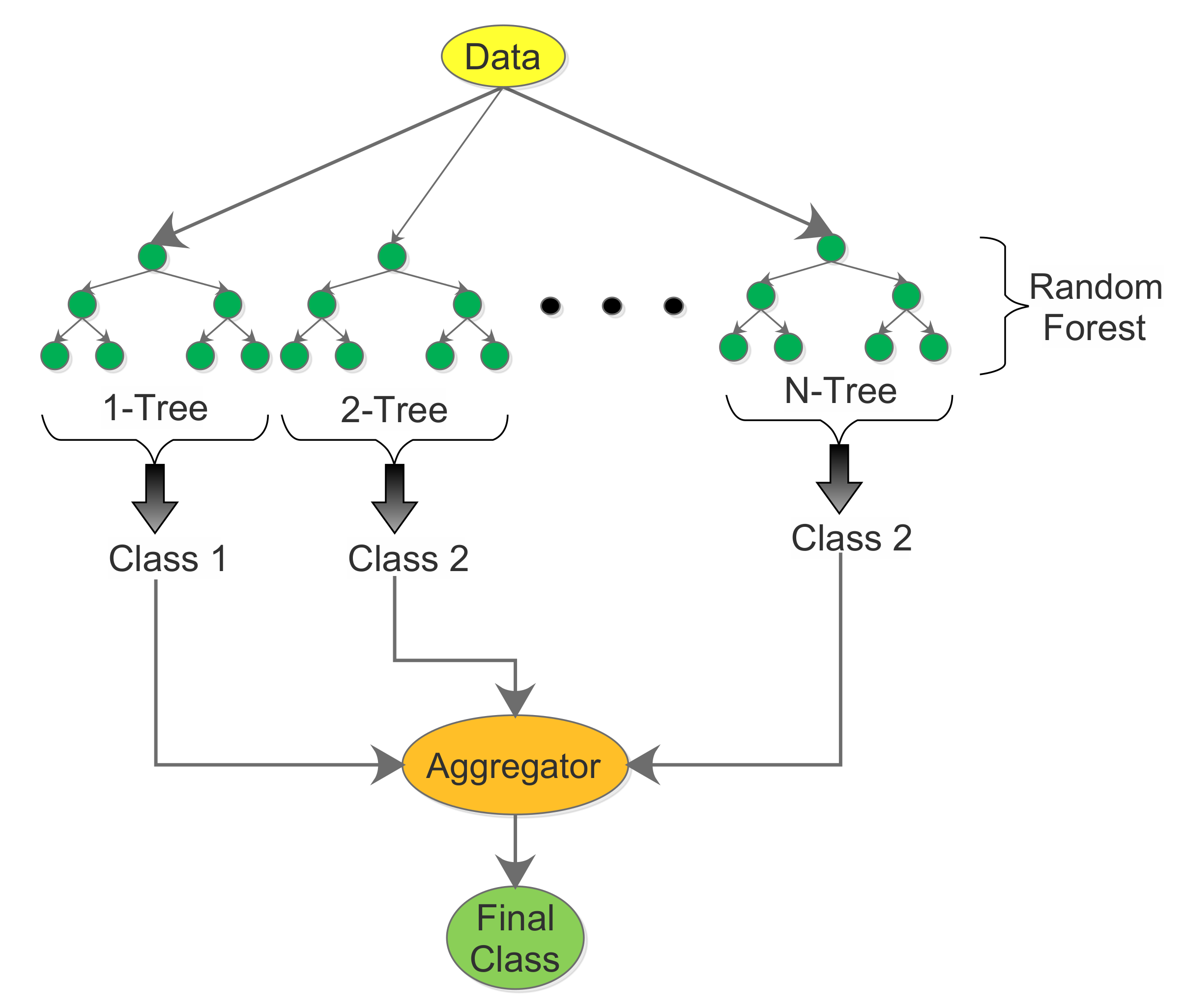
3.1.4. Random Forest

The RF is an ensemble of decision trees used for performing both regression and classification tasks [37]. It is built on the basis of the decision tree algorithm, which is capable of fitting complex datasets. The concept of the tree is to search for a variable–value pair within the training set and then to split this to obtain the best two child subsets. Essentially, when making predictions, each data point begins at the top of the tree (as shown in Figure 2) and then down through the branches until it reaches a leaf node, where no further branching can be achieved.
Being an ensemble approach, the RF aggregates multiple outputs generated via different sets of decision trees toward obtaining better results. The idea is to take an average over the outcome of each predictor, thus reducing the variance toward arriving at a better prediction model that presents fewer cases of overfitting the training data [38]. Thus, the RF becomes a strong learner, whereas the individual decision trees are considered weak learners. The RF algorithm is trained via the bagging method or bootstrap aggregating approach, which comprises randomly sampling subsets of the training data [39]. It then fits the model to these smaller datasets and then aggregates the predictions. This approach allows for many instances to be used repeatedly during the training phase. Essentially, the RF can be a slow algorithm since it has to grow many trees during the training stage. Further technical details regarding the RF algorithm can be accessed in [37]. The fine-tuned hyperparameters of the RF algorithm include the maximum depth and the number of iterations.

3.1.5. Support Vector Machine

The SVM aims to determine a hyperplane in an N-dimensional space, where N is the number of features, which distinctly classifies the data points [40]. The SVM is a generalized version of the maximal margin classifier, with provision for more data types to be better classified. Essentially, the SVM uses the hyperplane to separate optimally two convex hulls of points (data instances), by ensuring that the hyperplane is equidistant from the two convex hulls.
In this situation, the hyperplane is a classification border. It is usually a N 1 dimensional flat affine subspace, which is a line in two dimensions and a plane in three dimensions [41]. In terms of classification, the goal is to find the plane that optimizes the distance between two classes of data points. The hyperplane’s size depends on the number of features. In the SVM domain, support vectors are data points on or near the hyperplane. Using these support vectors allows us to optimize the hyperplane’s margin. They are called support vectors because any change in their position affects the hyperplane.
For non-linearly separated data points, the SVM adopts the concept of kernels to classify such points. A kernel refers to a function that maps lower dimensional data into higher dimensional ones. The function takes two vectors of any dimension as input and outputs a score (a dot product) that quantifies how similar the input vectors are. If the dot product is small, then the vectors are different, whereas if they are large, the vectors are similar. The SVM can use a variety of kernel functions, but one popular kernel is the Gaussian radial basis function (RBF). The RBF Gaussian kernel K ( x , y ) is calculated as follows:
K ( x , y ) = exp | | x 2 y 2 | | 2 2 σ 2
where x and y are N-dimensional independent variables, and σ is assumed to be the standard deviation of x and y, with | | | | being the Euclidean norm. Further formal and detailed explanation and use of the SVM can be obtained in [42,43], with the following hyperparameters fine tuned in the present study, namely, the kernel and filter type.

3.2. Dataset

We considered the system hourly demand and renewable power generation data obtained from the Eskom database in our study (https://www.eskom.co.za/dataportal/, accessed on 1 October 2021). Eskom is a South African electricity public utility company established to be the Electricity Supply Commission [44]. It owns and operates a number of noteworthy power plants that provide roughly 95% of South Africa’s electricity [45]. Eskom provides data on power generated, consumed, and from open cycle gas turbines, renewables and power outages. Our research focused on demand-side data and renewable energy sources, which are reflective of a typical smart grid. Thus, the use cases are as follows:
1.
System hourly demand: This dataset presents the hourly power demand measured from 5 to 18 October 2021 (https://www.eskom.co.za/dataportal/demand-side/system-hourly-actual-and-forecasted-demand/, accessed on 1 October 2021). It is classed into the residual and the Republic of South Africa (RSA) contracted demand. However, we considered only the residual demand data in our study, which suffices to compare the different algorithms. The entire dataset comprised 528 data points, with the residual demand data comprising 336 data points collated from 5 to 10 October 2021, and 192 data points from the residual forecast dataset provided from 11 to 18 October 2021. In this case, a training to testing split ratio of 65% to 35% was used, respectively.
2.
Hourly renewable generation: This dataset presents the hourly renewable generation per resource type, namely, from photovoltaic (PV) and wind sources (https://www.eskom.co.za/dataportal/renewables-performance/hourly-renewable-generation/, accessed on 1 October 2021). These datasets reflect only renewable sources owned by Eskom or that Eskom has contracts with. The PV and wind datasets comprised 960 data points in total, each measured per hour from 1 September 2021 to 10 October 2021. For both the PV and wind use cases, we used 80% of the dataset for training and 20% for testing. This implies that 770 data points from 1 September 2021 to 2 October 2021 were used to train each model, whereas 190 data points from 3 to 10 October 2021 were used for testing purposes. It should be noted that the term “target” used henceforth in this article refers to the actual data against which the different models are compared with during the testing phase.
The above use cases were selected because a typical grid-tied microgrid in a smart grid system can be expected to supply power to consumers both from the main grid as well as from local renewable sources. Consequently, when in the grid-tied mode, the system hourly actual demand dataset suffices as a relevant use case for prediction purposes. On the other hand, when in an island mode, the hourly renewable generation dataset becomes relevant for forecasting sake. Thus, both use cases are useful for designing energy management systems capable of day-ahead or week-ahead demand and supply forecasting in smart grids. Such knowledge helps to anticipate the amount of electricity that will be used hourly so that sufficient generation can be made available to meet such electricity demand.

3.3. Performance Metrics

As noted in Section 1, the possibility for bias arises when only a few metrics are reported while other notable metrics remain unreported [3]. Since each metric reports different information regarding an algorithm’s performance, some articles tend to only report those metrics that reflect their method’s improved performance while shunning others. However, to avoid such unacceptable practices, we used a variety of notable metrics to compare the different models with aim to provide a broader perspective regarding the performance of the different models. To this effect, five well-known evaluation metrics were considered, and they are discussed as follows.

3.3.1. Correlation Coefficient

The Pearson correlation coefficient (CC) r x y can be computed for any model as follows
r x y = i = 1 n ( x i x ¯ ) ( y i y ¯ ) i = 1 n ( x i x ¯ ) 2 i = 1 n ( y i y ¯ ) 2
where n is the sample size, x i , y i are the individual sample points (i.e., paired instances) indexed with i for a pair of random variables ( X , Y ) , and
x ¯ = 1 n i = 1 n x i
is the sample mean for X and similarly obtained for Y as follows
y ¯ = 1 n i = 1 n y i
Essentially, the value of r x y ranges from −1 to 1, where a value of 1 means that the relationship between X and Y can be described by a linear equation. In this case, all data points fall on a line. The correlation sign (− or +) follows from the regression slope, where a + sign means that Y increases as X increases and vice versa for a − sign. The case of r x y = 0 means that no correlation exists between X and Y. Other intermediate values (i.e., 0 < r x y < 1 and 1 < r x y < 0 ) describe partial correlations with values closer to 1 or −1 representing a better model based on the context and purpose of the experiment.

3.3.2. Relative Absolute Error

The relative absolute error (RAE) is the ratio of the total absolute error produced by a model to the total absolute error of a simple predictor. In this case, the simple predictor is just the average of the target values. The RAE is thus computed as
R A E = i = 1 n | P i A i | i = 1 n | A ¯ A i | × 100 %
where P i is the predicted value by a model for an instance i out of a total number of n instances, A i is the target value for the instance i, and A ¯ is the mean of the target values given by
A ¯ = 1 n i = 1 n A i
One advantage of the RAE metric compared to the root mean square error (RMSE) described later is that it treats each error equally by ensuring that only the absolute value is considered and not the square of the error. Consequently, systems that are invariant to the effects of outliers can be best evaluated by the RAE instead of the RMSE.

3.3.3. Root Relative Square Error

The root relative square error (RRSE) is the ratio of the square root of the sum of the squared errors to the sum of the squared errors of a simple predictor. Again, the simple predictor is the average of the target values. The RRSE is given as
R R S E = i = 1 n ( P i A i ) 2 i = 1 n ( A ¯ A i ) 2 × 100 %
where all terms remain as previously defined. By computing the square root of the relative squared error, the RRSE reduces the error to a similar magnitude range as the RAE. However, unlike the RAE, the RRSE penalizes outliers with large error values, thus allowing models with plausible outliers to be easily identified.

3.3.4. Mean Absolute Error

The mean absolute error (MAE) is a measure of the error between a pair of random variables expressing the same event. It is computed as
M A E = 1 n i = 1 n | P i A i |
Following (13), it can be observed that an errorless model will generate a zero MAE value, since P i = A j , thus indicating that the MAE ranges from 0 to infinity, with 0 being an ideal model. For this reason, the MAE is a boundless metric and thus, is data specific. Nevertheless, it remains a valuable metric for comparing models that are based on the same input data.

3.3.5. Root Mean Square Error

The root mean square error (RMSE) is a measure of accuracy for comparing the forecast errors of different models based on the same dataset. It is the square root of the average of the squared errors, mathematically computed as follows
R M S E = i = 1 n ( P i A i ) 2 n .
Since computing the RMSE involves squaring the difference between the predicted and the target values, thus, a few large differences will definitely increase the RMSE compared to the MAE. Consequently, the RMSE is sensitive to outliers, and hence useful for analyzing models with outlier tendencies.

4. Results and Discussion

In this section, we present and discuss both quantitative and qualitative results obtained from the evaluation and analysis of the ML models considered in our study. By quantitative analysis, we present and discuss the evaluation metrics as they relate to the performance of the different models. By qualitative analysis, we refer to the visual assessment of the different displays of the predicted against the target values of the different models. To this effect, firstly, we conducted a parameter tuning exercise toward ensuring that all models are evaluated based on their best parameter values. For this purpose, the GridSearchCV tool was used with discrete sets of parameter values designated per model. The system hourly demand dataset was used for the fine-tuning process. Thereafter, the fine-tuned models were tested and compared based on the hourly renewable generation dataset, and the results are discussed. The models were simulated using the Waikato Environment for Knowledge Analysis platform upon on a computer having an i7-10750H central processing unit and an NVIDIA GeForce GTX 1650 Ti GPU.

4.1. Hyper-Parameter Optimization

4.1.1. Artificial Neural Network

ANN algorithms are typically characterized by a number of hyperparameters that should be properly fine tuned to obtain models that perform optimally. These hyperparameters are the number of neurons, activation function, learning rate, momentum, batch size, and epochs. However, since the hyperparameter tuning procedure can be a cumbersome and time-consuming process, consequently, we used the sigmoid as the activation function and we kept the batch size fixed for all methods at 100, whereas the epoch was fixed at 500. All other hyperparameters were then fine tuned accordingly.
Table 2 presents the different parameter settings and their respective performances based on the CC, RAE, and RRSE. The number of hidden layers and nodes per layer is denoted as ( x 1 , x 2 , , x n ) , where the number of elements (i.e., index) n represents the number of hidden layers, while the value of each element denotes the number of nodes per layer. Essentially, we examined a maximum of two hidden layers with the number of nodes per hidden layer increased from 6, 9, to 12. We then considered three states for the learning rate classed as low (0.1), medium (0.3), and high (0.5). For the momentum parameter, we examined three values at 0.1, 0.2, and 0.4. These values were selected to understand how the model performs under increasing or decreasing values. The following are our findings.
1.
The model’s performance typically decreases under an increased learning rate and momentum values, irrespective of the number of hidden layers used. This implies that a low learning rate and momentum values are best suitable for an ANN model, with the values of 0.1 and 0.1 yielding the lowest error rates, respectively. This can be easily explained noting that low learning rate values imply smaller step sizes and thus higher resolutions, which leads to improved convergence to better approximations.
2.
A model with two hidden layers with 12 nodes per layer yielded the lowest error rates under a low learning rate and momentum values. Although this configuration cannot be generalized for all ANN models, it yielded the lowest error rate for the present use case. Furthermore, we note that increasing the number of nodes above 12 produced no improvement in model performance.
3.
Generally, under the same low learning rate and momentum values, we observed that the double-layered model performed marginally better than the single layer configuration. For example, considering in Table 2 the best model of (12,12) hidden layer configuration, and learning rate and momentum of 0.1 each, we obtained a 2.155 % decrease in the error rate when using the double-layered model instead of the single-layered model of same number of nodes.
4.
Since there is no single fixed global configuration or model for all possible use cases, it becomes vital to ensure that a model’s hyperparameters are accurately fine tuned. For example, by fine tuning our model, we achieved a 10.344 % error reduction rate in using a double-layer model with 12 nodes per layer (learning rate = 0.1, momentum = 0.1) over a single-layer model with 9 nodes (learning rate = 0.3, momentum = 0.2).

4.1.2. Gaussian Regression

The following hyperparameters of the GR algorithm were fine tuned, namely, the kernel and the filter type. The kernels considered were the polynomial (poly) kernel, radial basis function (RBF), and the normalized polynomial kernel. The filter types included either the normalization or standardization of the training data. Our findings from the results in Table 3 are noted as follows:
1.
A combination of the poly kernel and standardization of the training data led to the best model, which yielded the lowest RAE and RRSE values of 44.7277% and 45.5645%, respectively.
2.
Hyperparameter tuning of the GR algorithm can achieve as much as 51.387 % and 50.301 % error reduction rate in the RAE and RRSE, respectively, thus emphasizing the importance of hyperparameter tuning.
3.
With R A E and RRSE differences of 3.121% and 3.645%, respectively, there exists little/no significant advantage in using either the normalization or standardization of the training data as it pertains to the poly kernel. Consequently, the most important parameter is simply the choice of the kernel to be used.
4.
We presume that the RBF kernel may have performed poorly owing to the large size of the training dataset, which is a well-known limitation of the RBF. Nevertheless, it is noted that performance improvement can yet be achieved by standardizing the training data.

4.1.3. k-Nearest Neighbor

The k-NN algorithm is characterized by one major parameter, which is the k parameter. The neighbor search method is another parameter; however, the linear search approach based on the Euclidean distance metric was used in our study. The following k values were selected as k = 1 , 3 , 5 , and 10. The results obtained are presented in Table 4.
We observed that the same error rate (i.e, RAE and RRSE values) was obtained for parameters k = 1 , 3 , and 5. At k = 10 , a large error rate of 100 % was realized, thus implying that large K values are inappropriate for use under the present use case. With lower k values yielding the same results, it is suitable to use k = 1 since it presents the least computational demand for the model.

4.1.4. Linear Regression

The linear regression (LR) method can be improved based on the choice of the attribute selection method. We tested the LR algorithm without any attribute selection method, as well as with the M5 and greedy attribute selection method. The results obtained are presented in Table 5 with little or no difference between the different selection methods. Using an attribute selection method achieved only about 0.764% reduction in the error rate over the use of the no-selection method. Thus, for power demand prediction purposes, it is sufficient to apply the LR method without any attribute selection method. This is expected since there exist only the day and time as the main input attributes for forecasting purposes, thus attribute selection introduces no significant performance advantage.

4.1.5. Random Forest

The random forest (RF) algorithm has a few parameters to be fine tuned, namely, the maximum depth and the number of iterations. In our study, a combination of three parameters were examined with progressively increasing values and the results obtained are presented in Table 6. We found that increasing the maximum depth and number of iterations barely resulted in 0.409% and 0.378% decreases in the RAE and RRSE error rates, respectively. This insignificant difference in the error rate implies that using low maximum depth values and number of iterations will be suitable in using the RF algorithm for power demand prediction purposes. It also may present faster computational time since fewer iterative steps are considered during the algorithmic process.

4.1.6. Support Vector Machine

The support vector machine (SVM) algorithm was optimized by tuning the kernel and filter type parameters to improve its performance. The results obtained are presented in Table 7. We found that a combination of the poly kernel and the normalization of the training data resulted in the least error rates across both RAE and RRSE. In this case, both the polynomial and normalized polynomial kernel combined with normalization of the training data achieved the same performance. However, we note that it will be of greater value computation wise to avoid the normalization expenses of the poly kernel, thus implying that using the simple poly kernel should suffice for the present case. Similar to the GR algorithm, the RBF kernel yielded the largest error rates with the same plausible reasons as stated for the GR algorithm applying as well to the SVM algorithm. Summarily, an average of 38.15% reduction in the error rate was achieved by using the poly kernel over the RBF, thus reemphasizing the importance of hyperparameter tuning in the use of ML algorithms.

4.1.7. Comparison of the Different Methods

Following the hyperparameter tuning process, the best performing models of the different algorithms were compared, and the results obtained are presented in Table 8. To this effect, the following metrics were compared across the different models, namely CC, RAE, RRSE, MAE, and RMSE. Our findings indicate that although it may seem that some algorithms performed better than others, nevertheless, the performance gap suffices only marginally. For example, there existed only a 1.899% reduction in the error rate in using the ANN over the GR model in terms of their RAE. A difference of about 3.553% in the RRSE existed between the SVM and the RF algorithm. Thus, suggesting an insignificant difference between the different models, sequel to a proper hyperparameter tuning process.
No model performed best across all the different metrics, thus emphasizing the need to avoid comparing different ML models using only a single metric. For example, although the ANN performed best considering the RAE, it generated the smallest RRSE values compared to the other models. Since these different metrics tell different stories, it is essential to consider our analysis across each metric as against a single metric. To this effect, by rendering a higher RRSE value, we note that the ANN model may have been plagued by more outliers than the other methods. This observation is again supported by examining the MAE against the RMSE in Table 8, which shows a higher RMSE than other methods, except the SVM.
In addition, we examined the CC values of the different models, with results of the correlation matrix presented in Figure 3. By comparing the CC achieved by the different models against the target demand, we observed that a C C < 0.9 was obtained across all models. This implies a good positive correlation between the predicted and the target demand values. In addition, we can observe that a C C 1 was obtained between the different models, further emphasizing that the different models all predicted the same values. In particular, the ANN, GR, KNN and RF models all performed equally with little to distinguish them.
Finally, in quantitative terms, a Tukey comparative test of the different models was performed, and the output results are documented in Table 9. The Tukey test is a multiple comparison procedure that can be used to find means that are significantly different from each other. The aim in using this test is to quantitatively determine whether there exists a significant difference between the mean results obtained across the different models or not. Further details regarding the Tukey test can be accessed in [46]. The symbols used to interpret the range of the p-values, p, obtained for all the Tukey tests reported in this article, are provided in Table 10. An examination of Table 9 indicates that there was no significant (ns) difference between the target and predicted data of the different models (see column 5 of Table 9). It also confirms that there was no significant difference between all other methods as well, with p-values all averagely being greater than 0.997. These results support the correlation findings of Figure 3, further emphasizing that following a proper hyperparameter tuning exercise of the different algorithms, they all perform, on average, the same, with little or no significant difference between them.

4.1.8. Visual Assessment of Predicted Values of the Different Methods

Figure 4 presents the target and predicted values generated by the different models. It is immediately obvious that the graphs are practically overlapped, which further confirms that the models achieved similar performance levels. Essentially, there was only very little difference between the predictive values and the target data prior to the 120th h (i.e., day 5), beyond which a significant error difference was observed. This can be explained noting that a stable pattern existed within the first 5 days, followed by some drop in the target demand level between the 6th and 7th day (i.e., from 120 to 168 h), a period which was not properly tracked by the different methods. This implies that the different ML methods may perform best under conditions with well-defined patterns, and otherwise under heavy stochastic conditions.

4.2. Hourly Renewable Generation

In this section, we discuss our findings pertaining to the photovoltaic (PV) and wind hourly generation datasets. We note that the best-performing models obtained in the hyperparameter tuning section were used here.

4.2.1. Photovoltaic Generation

The performance results of the different models based on the PV dataset are presented in Table 11. In terms of the CC, although the GR model achieved only a slightly higher margin (<0.001) than the ANN and LR models, we can easily conclude that there was no significant difference between the different models. This implies that the predicted results are highly positively correlated with the target demand. Similar high CC values were also obtained between the different models as shown in the correlation matrix of Figure 5. Therein, it can be seen that only the k-NN and RF models had slightly lower CC values to the other models. This may be because both models achieved the lowest CC value as against the target demand. Nevertheless, for use cases where only the data pattern suffices as the main interest to the designer, then any ML method can be used.
By examining the error performance of the different models via the RAE and RRSE in Table 11, it can be observed that the ANN performed the poorest. Thus, it can be said that a 25.503 % decrease in the RAE can be achieved by using the k-NN instead of the ANN for the PV power prediction use case. Although this seems large, nevertheless, further analysis following the Tukey comparative test suggests that there was no significant difference between the predicted means of the different models. This can be seen in Table 12, where it is concluded that there was no significant difference in the predicted means of the different models. Thus, this suggests that any model may suffice for PV power forecasting purposes sequel to a proper hyperparameter tuning exercise.
Finally, a visual assessment of the predicted against the target PV generation results is presented in Figure 6. Here, it is observed that a close performance was achieved between the predicted values of the different models and the target data. The overlapping graphs in Figure 6 also confirm that the models all performed similarly with little to distinguish them visually. Since the pattern obtained for PV generation demonstrates strong regularity with peak generation often obtained during midday (at peak sunshine), consequently any model can be used for predictive purposes, typically after properly tuning the model’s hyperparameters.

4.2.2. Wind Generation

The performance of the different models based on the wind power generation dataset is presented in Table 13. It is immediately clear that the models performed poorly under this use case, with each model particularly suffering from very high error rates and low CC values. Albeit low, it is also seen that the CC values are, on average, the same for the models when compared to the target data. However, high and positive CC values are obtained when compared between the different models as shown in the correlation matrix of Figure 7. This confirms that the different models all performed similarly with almost perfect correlation between their predicted values.
The error rates as measured via the RAE and RRSE indicate that the ANN generated the highest error rate, and thus is reported as the poorest performer. Essentially, the RRSE values of each model return higher than their corresponding RAE values, which indicates the presence of outliers across the different models under the wind prediction use case. On the other hand, the SVM model suffices as the best performer, as it achieved a 21.18 % reduction in the RAE as compared with the ANN model.
A Tukey test was conducted to examine the differences in the mean values of the models, and the results obtained are presented in Table 14. We observed that, unlike in the PV power prediction and the system hourly demand datasets, there was a significant difference in the mean performance of the different models and the target data. This can be seen in column 4 of Table 14 with very low associated p-values, where the performance of the ANN model is also indicated to be significantly different from all other models.
Finally, a visual assessment of the predicted values of the different models can be made, based on the results of Figure 8. We observed that the different models only matched the rising patterns of the target data while failing to track periods of low wind power generation. This implies that the inherent irregularities in the wind power generation pattern typically limited the output performance of the different models. We also observed that the predicted values of the ANN model deviated largely from the target as well as from the other models, thus justifying its poor performance as noted in Table 13 and Table 14. Consequently, because of the highly stochastic nature of wind, it may be difficult to apply ML models for predicting wind power generation, thus warranting the need for improved methods in this regard.

4.2.3. Runtime Performance of the Different Algorithms

We performed a runtime evaluation of the various algorithms on both the PV and wind datasets, and the results are shown in Table 15. To begin, it is important to note that the following conditions were met prior to conducting these experiments:
1.
The same datasets (i.e., PV and wind data) were used to evaluate each algorithm.
2.
Both the training and testing runtime performance was measured and reported.
3.
To ensure that no extra processing time was incurred by the PC, only the simulation software was kept running as the foreground process during each simulation period. This was accomplished by closing all other foreground processes in the PC’s task manager.
4.
Finally, the timing results shown in Table 15 were obtained by averaging the results of 50 independent runs of each algorithm.
Table 15 shows the empirical run-time results of each algorithm. However, it should be noted that because the k-NN is an unsupervised method, there was no need for a training process, and thus, no results are provided for it. According to these results, the LR achieved the shortest training time in both datasets, while the SVM algorithm achieved the quickest testing time in the PV dataset while having the same testing time as the ANN and LR in the wind dataset. Often, because testing time is most important to the user during real-time operation, we note that the SVM performed best; however, statistical significant analysis of these timing results shows otherwise in Table 16.
It should be noted that only the test time results of Table 15 for both the PV and wind datasets were subjected to the Tukey statistical test. Thus, the Tukey test results in Table 16 reveal that there were no statistically significant (ns) differences in the test time of the different algorithms, albeit for the GR algorithm, which yielded the longest test time compared to the other methods. The GR algorithm’s relatively slower performance may be attributed to the effect of the Gaussian kernel, which is known to add additional processing requirements to the method. However, because the difference in the testing time performance was less than 0.195 s across all methods (see column 2 of Table 16), it is possible to conclude that any of these algorithms can be used for real-time power demand/supply prediction use cases in smart grid systems.

5. Conclusions

The goal of this study was to determine whether there is a statistically significant difference in the performance of various well-known simple machine learning (ML) models when they are applied to the prediction of power demand and supply. In order to accomplish this, six well-known machine learning methods were tested using data from the Eskom database, which included hourly system demand and renewable generation datasets. The ML algorithms considered include the artificial neural network, Gaussian regression, K-nearest neighbor, linear regression, random forest, and the support vector machine, among other methods of data analysis. Fairness was achieved by ensuring that the hyperparameters of each algorithm were fine tuned to the greatest degree possible. Our findings suggest that, within the confines of the datasets used in this study, there was little/no statistically significant difference between the different models in terms of both quantitative and qualitative measures, which is particularly noteworthy, given that they were all meticulously fine tuned. Additionally mentioned is the importance of reporting as many metrics as possible, particularly the correlation coefficient and absolute and squared errors, in order to ensure that fair conclusions are formed when comparing different machine learning algorithms. Based on the fact that each metric often reports a separate performance measure and that selective reporting may result in erroneous conclusions, this requirement is recommended. Furthermore, when it came to estimating the wind power generation dataset, all of the models performed poorly, which we attributed to the extremely stochastic nature of wind energy as a source of energy, as previously stated in the literature. This may imply that improved models for smart grid systems may be required, particularly in areas where wind power constitutes a significant portion of the generated electricity. In spite of this, it is possible that any ML model can still be used for power prediction in smart grid systems, particularly in situations where demand and generation follow regular patterns, and provided that the model’s hyperparameters are properly tuned based on the type of input data being used. Finally, we stress that further robust investigations, particularly those based on the use of larger datasets from a wider range of sources, should be strongly encouraged in order to either substantiate or refute the conclusions of the present paper.

Author Contributions

These authors E.C., A.J.O. and S.J.I. contributed equally to this work. Conceptualization, A.J.O., E.C. and S.J.I.; methodology, E.C. and A.J.O.; writing—original draft preparation, A.J.O. and E.C.; writing—review and editing, A.J.O. and S.J.I.; supervision, A.J.O. and S.J.I.; funding acquisition, S.J.I. All authors have read and agreed to the published version of the manuscript.

Funding

This research was funded by the COUNCIL FOR SCIENTIFIC AND INDUSTRIAL RESEARCH (CSIR) with project number 05400 054AT KR2EEMG. and The APC was funded by project number 05400 054AT KR2EEMG.

Institutional Review Board Statement

Not applicable.

Informed Consent Statement

Not applicable.

Data Availability Statement

Not applicable.

Conflicts of Interest

The authors declare no conflict of interest. The funders had no role in the design of the study; in the collection, analyses, or interpretation of data; in the writing of the manuscript; or in the decision to publish the results.

Abbreviations

The following abbreviations are used in this article:
ANNArtificial neural network
CCCorrelation coefficient
ELMExtreme learning machine
EPNEnsemble prediction network
FFANNFeed-forward artificial neural network
GRGaussian regression
KELMKernel-based extreme learning machine
k-NNk-nearest neighbor
LRLinear regression
LSTMLong short-term memory
MAEMean absolute error
MLMachine learning
MLPMultilayer perceptron
MSEMean square error
MVRMulti-variable regression
PVPhotovoltaic
RAERelative absolute error
RBFRadial basis function
RFRandom forest
RMSERoot mean square error
RRSERoot relative square error
RSARepublic of South Africa
RSSResidual sum of squares
SASimulated annealing
SVMSupport vector machine
WTWavelet transform
[ ] Brackets
( ) Parentheses
Square root
dy/dxDerivative
| | | | Euclidean norm
Summation
| | Absolute value

References

  1. Danish, M.S.S.; Senjyu, T.; Funabashia, T.; Ahmadi, M.; Ibrahimi, A.M.; Ohta, R.; Howlader, H.O.R.; Zaheb, H.; Sabory, N.R.; Sediqi, M.M. A sustainable microgrid: A sustainability and management-oriented approach. Energy Procedia 2019, 159, 160–167. [Google Scholar] [CrossRef]
  2. Nespoli, A.; Ogliari, E.; Pretto, S.; Gavazzeni, M.; Vigani, S.; Paccanelli, F. Electrical Load Forecast by Means of LSTM: The Impact of Data Quality. Forecasting 2021, 3, 91–101. [Google Scholar] [CrossRef]
  3. Lago, J.; Marcjasz, G.; Schutter, B.D.; Weron, R. Forecasting day-ahead electricity prices: A review of state-of-the-art algorithms, best practices and an open-access benchmark. Appl. Energy 2021, 293, 1–21. [Google Scholar] [CrossRef]
  4. Hong, T.; Pinson, P.; Wang, Y.; Weron, R.; Yang, D.; Zareipour, H. Energy Forecasting: A Review and Outlook. IEEE Open Access J. Power Energy 2020, 7, 376–388. [Google Scholar] [CrossRef]
  5. Uniejewski, B.; Weron, R.; Ziel, F. Variance Stabilizing Transformations for Electricity Spot Price Forecasting. IEEE Trans. Power Syst. 2018, 33, 2219–2229. [Google Scholar] [CrossRef] [Green Version]
  6. Marcjasz, G.; Uniejewski, B.; Weron, R. On the importance of the long-term seasonal component in day-ahead electricity price forecasting with NARX neural networks. Int. J. Forecast. 2019, 35, 1520–1532. [Google Scholar] [CrossRef]
  7. Wang, L.; Zhang, Z.; Chen, J. Short-Term Electricity Price Forecasting with Stacked Denoising Autoencoders. IEEE Trans. Power Syst. 2017, 32, 2673–2681. [Google Scholar] [CrossRef]
  8. Ugurlu, U.; Oksuz, I.; Tas, O. Electricity Price Forecasting Using Recurrent Neural Networks. Energies 2018, 11, 1255. [Google Scholar] [CrossRef] [Green Version]
  9. Chen, Y.; Wang, Y.; Ma, J.; Jin, Q. BRIM: An Accurate Electricity Spot Price Prediction Scheme-Based Bidirectional Recurrent Neural Network and Integrated Market. Energies 2019, 12, 2241. [Google Scholar] [CrossRef] [Green Version]
  10. Rijn, J.N.; Hutter, F. Hyperparameter Importance Across Datasets. In Proceedings of the 24th ACM SIGKDD International Conference on Knowledge Discovery & Data Mining, London, UK, 19–23 August 2018; pp. 2367–2376. [Google Scholar] [CrossRef] [Green Version]
  11. Bhotto, M.Z.A.; Jones, R.; Makonin, S.; Bajic, I.V. Short-Term Demand Prediction Using an Ensemble of Linearly-Constrained Estimators. IEEE Trans. Power Syst. 2021, 36, 3163–3175. [Google Scholar] [CrossRef]
  12. Muni, S.P.; Sharma, R. Short-term electricity price prediction using kernel-based machine learning techniques. In Proceedings of the 2021 1st Odisha International Conference on Electrical Power Engineering, Communication and Computing Technology (ODICON), Bhubaneswar, India, 8–9 January 2021; pp. 1–5. [Google Scholar] [CrossRef]
  13. Li, Y.; Wang, R.; Yang, Z. Optimal Scheduling of Isolated Microgrids Using Automated Reinforcement Learning-Based Multi-Period Forecasting. IEEE Trans. Sustain. Energy 2022, 13, 159–169. [Google Scholar] [CrossRef]
  14. Shi, Z.B.; Li, Y.; Yu, T. Short-Term Load Forecasting Based on LS-SVM Optimized by Bacterial Colony Chemotaxis Algorithm. In Proceedings of the 2009 International Conference on Information and Multimedia Technology, Beijing, China, 16–18 December 2009; pp. 306–309. [Google Scholar] [CrossRef]
  15. Sabzehgar, R.; Amirhosseini, D.Z.; Rasouli, M. Solar power forecast for a residential smart microgrid based on numerical weather predictions using artificial intelligence methods. J. Build. Eng. 2020, 32, 101629. [Google Scholar] [CrossRef]
  16. Scolari, E.; Sossan, F.; Paolone, M. Irradiance prediction intervals for PV stochastic generation in microgrid applications. Sol. Energy 2016, 139, 116–129. [Google Scholar] [CrossRef]
  17. Mohamed, M.; Chandra, A.; Abd, M.A.; Singh, B. Application of machine learning for prediction of solar microgrid system. In Proceedings of the 2020 IEEE International Conference on Power Electronics, Drives and Energy Systems (PEDES), Jaipur, India, 16–19 December 2020; pp. 1–5. [Google Scholar] [CrossRef]
  18. Onumanyi, A.J.; Isaac, S.J.; Kruger, C.P.; Abu-Mahfouz, A.M. Transactive Energy: State-of-the-Art in Control Strategies, Architectures, and Simulators. IEEE Access 2021, 9, 131552–131573. [Google Scholar] [CrossRef]
  19. Viel, F.; Silva, L.A.; Leithardt, V.R.Q.; Santana, J.F.D.P.; Teive, R.C.G.; Zeferino, C.A. An Efficient Interface for the Integration of IoT Devices with Smart Grids. Sensors 2020, 20, 2849. [Google Scholar] [CrossRef]
  20. Helfer, G.A.; Barbosa, J.L.V.; Alves, D.; da Costa, A.B.; Beko, M.; Leithardt, V.R.Q. Multispectral Cameras and Machine Learning Integrated into Portable Devices as Clay Prediction Technology. J. Sens. Actuator Netw. 2021, 10, 40. [Google Scholar] [CrossRef]
  21. Dalai, I.; Mudali, P.; Pattanayak, A.S.; Pattnaik, B.S. Hourly prediction of load using edge intelligence over IoT. In Proceedings of the 2019 11th International Conference on Advanced Computing (ICoAC), Chennai, India, 18–20 December 2019; pp. 117–121. [Google Scholar] [CrossRef]
  22. Ma, Y.J.; Zhai, M.Y. Day-Ahead Prediction of Microgrid Electricity Demand Using a Hybrid Artificial Intelligence Model. Processes 2019, 7, 320. [Google Scholar] [CrossRef] [Green Version]
  23. Dridi, A.; Moungla, H.; Afifi, H.; Badosa, J.; Ossart, F.; Kamal, A.E. Machine Learning Application to Priority Scheduling in Smart Microgrids. In Proceedings of the 2020 International Wireless Communications and Mobile Computing (IWCMC), Limassol, Cyprus, 15–19 June 2020; pp. 1695–1700. [Google Scholar] [CrossRef]
  24. Tian, W.; Lei, C.; Tian, M. Dynamic prediction of building HVAC energy consumption by ensemble learning approach. In Proceedings of the 2018 International Conference on Computational Science and Computational Intelligence (CSCI), Las Vegas, NV, USA, 12–14 December 2018; Volume 8, pp. 254–257. [Google Scholar] [CrossRef]
  25. Hajjaji, I.; Alami, H.E.; El-Fenni, M.R.; Dahmouni, H. Evaluation of Artificial Intelligence Algorithms for Predicting Power Consumption in University Campus Microgrid. In Proceedings of the 2021 International Wireless Communications and Mobile Computing (IWCMC), Harbin, China, 28 June–2 July 2021; pp. 2121–2126. [Google Scholar] [CrossRef]
  26. Kubat, M. Artificial Neural Networks. In An Introduction to Machine Learning; Springer International Publishing: New York, NY, USA, 2021; pp. 117–143. [Google Scholar] [CrossRef]
  27. Graupe, D. Principles of Artificial Neural Networks, 3rd ed.; Advanced Series in Circuits and Systems; World Scientific Publishers: Singapore, 2013; Volume 7, pp. 1–382. [Google Scholar] [CrossRef]
  28. Hajian, A.; Styles, P. Artificial Neural Networks. In Application of Soft Computing and Intelligent Methods in Geophysics; Springer International Publishing: New York, NY, USA, 2018; pp. 3–69. [Google Scholar] [CrossRef]
  29. Principe, J. Artificial Neural Networks. In Electrical Engineering Handbook; CRC Press: New York, NY, USA, 1997. [Google Scholar] [CrossRef]
  30. Pirjatullah; Kartini, D.; Nugrahadi, D.T.; Muliadi; Farmadi, A. Hyperparameter Tuning using GridsearchCV on The Comparison of The Activation Function of The ELM Method to The Classification of Pneumonia in Toddlers. In Proceedings of the 2021 4th International Conference of Computer and Informatics Engineering (IC2IE), Jakarta, Indonesia, 22–24 October 2021; pp. 390–395. [Google Scholar] [CrossRef]
  31. Fontenla-Romero, O.; Erdogmus, D.; Principe, J.C.; Alonso-Betanzos, A.; Castillo, E. Linear Least-Squares Based Methods for Neural Networks Learning. In Artificial Neural Networks and Neural Information Processing—ICANN/ICONIP 2003; Springer: Istanbul, Turkey, 2003; pp. 84–91. [Google Scholar] [CrossRef]
  32. Schulz, E.; Speekenbrink, M.; Krause, A. A tutorial on Gaussian process regression: Modelling, exploring, and exploiting functions. J. Math. Psychol. 2018, 85, 1–16. [Google Scholar] [CrossRef]
  33. Banerjee, A.; Dunson, D.B.; Tokdar, S.T. Efficient Gaussian process regression for large datasets. Biometrika 2013, 100, 75–89. [Google Scholar] [CrossRef]
  34. Gramacy, R.B. Gaussian Process Regression. In Surrogates; Chapman and Hall/CRC: London, UK, 2020; pp. 143–221. [Google Scholar] [CrossRef]
  35. Cunningham, P.; Delany, S.J. k-Nearest Neighbour Classifiers - A Tutorial. ACM Comput. Surv. 2021, 54, 1–25. [Google Scholar] [CrossRef]
  36. Ali, N.; Neagu, D.; Trundle, P. Evaluation of k-nearest neighbour classifier performance for heterogeneous data sets. SN Appl. Sci. 2019, 1, 1–5. [Google Scholar] [CrossRef] [Green Version]
  37. Biau, G.; Scornet, E. A random forest guided tour. TEST 2016, 25, 197–227. [Google Scholar] [CrossRef] [Green Version]
  38. Probst, P.; Boulesteix, A.L. To tune or not to tune the number of trees in random forest? J. Mach. Learn. Res. 2017, 18, 1–18. [Google Scholar]
  39. Probst, P.; Wright, M.N.; Boulesteix, A. Hyperparameters and tuning strategies for random forest. WIREs Data Min. Knowl. Discov. 2019, 9, e1301. [Google Scholar] [CrossRef] [Green Version]
  40. Yang, X.S. Support vector machine and regression. Chapter Support vector machine and regression. In Introduction to Algorithms for Data Mining and Machine Learning; Yang, X.S., Ed.; Elsevier: Amsterdam, The Netherlands, 2019; pp. 129–138. [Google Scholar] [CrossRef]
  41. Pisner, D.A.; Schnyer, D.M. Support vector machine. In Machine Learning; Elsevier: Amsterdam, The Netherlands, 2020; pp. 101–121. [Google Scholar] [CrossRef]
  42. Suthaharan, S. Support Vector Machine. In Machine Learning Models and Algorithms for Big Data Classification; Springer: New York, NY, USA, 2016; pp. 207–235. [Google Scholar] [CrossRef]
  43. Cervantes, J.; Garcia-Lamont, F.; Rodríguez-Mazahua, L.; Lopez, A. A comprehensive survey on support vector machine classification: Applications, challenges and trends. Neurocomputing 2020, 408, 189–215. [Google Scholar] [CrossRef]
  44. Mondi, L. Eskom: Electricity and technopolitics in South Africa by Syvly Jaglin, Alain Dubresson. Transform. Crit. Perspect. South. Afr. 2017, 93, 176–185. [Google Scholar] [CrossRef]
  45. Roy-Aikins, J. Challenges in Meeting the Electricity Needs of South Africa. In Proceedings of the ASME 2016 Power Conference, Charlotte, NC, USA, 26–30 June 2016. [Google Scholar] [CrossRef]
  46. Lee, S.; Lee, D.K. What is the proper way to apply the multiple comparison test? Korean J. Anesthesiol. 2018, 71, 353–360. [Google Scholar] [CrossRef] [PubMed] [Green Version]
Figure 1. Representations of an ANN: (a) Single-layer (b) Multi-layer.
Sustainability 14 02546 g001
Figure 2. A representation of the concept of the random forest algorithm.
Sustainability 14 02546 g002
Figure 3. The correlation matrix of the different methods for the system hourly demand dataset.
Sustainability 14 02546 g003
Figure 4. System hourly demand: target demand compared against the predicted demand generated by the different models using their best hyper-parameter values.
Sustainability 14 02546 g004
Figure 5. The correlation matrix of the different methods for the photovoltaic power generation dataset.
Sustainability 14 02546 g005
Figure 6. Photovoltaic power generation: Target and predicted demand generated by the different models.
Sustainability 14 02546 g006
Figure 7. The correlation matrix of the different methods for the wind power generation dataset.
Sustainability 14 02546 g007
Figure 8. Wind generation: Target and predicted demand generated by the different models.
Sustainability 14 02546 g008
Table 1. Summary of the related studies, with key characteristics from each study compared to the others.
Ref.YearMethods
Compared
Metrics
of
Comparison
Was Statistical
Significance
Analysis
Performed?
Was
Processing
Time Measured?
Findings
[11]2021EPN, LSTM,
ANN
RMSE, MAPENoYes:
EPN was fastest
EPN outperformed LSTM, MLP, SVR and ETR in terms of RMSE over a wide variety of data
[12]2021ELM
Kernel-based technique
MAE, MAPE,
RMSE
NoNoKernel based methods performed better than ELM; Gaussian kernel performed better than other kernel methods.
[15]2020ANN, MVR,
SVM
MAPE, MSENoNoThe developed neural network model outperformed the MVR and SVM
[17]2020Regression,
ANN
MSE, RMSE,
R-squared
Chi-squared
NoNoRegression approach has a better performance than some state-of-the-art method such as feed forward neural network.
[21]2019LR, ANN,
SMO regression, SVM
MAE, RMSE,
CC
NoYes,
but only
for SVM
SVM performed better than other algorithms compared with.
[22]2019FFANN, WT,
SA
MAPE, RMSE,
NMAE
NoNoFFANN performed better than BP-, GA-, and PSO-FFANN schemes
[23]2020LSTMRMSE, MAENoNoNo comparison
[24]2018MLR, decision tree, RF,
Gradient boosted trees
ARENoNoGradient boosted trees performed better than others.
[25]2021ARIMA, SARIMA,
SVM, XGBoost,
RNN, LSTM,
LSTM-RNN
MAE, MAPE,
MSE, R-squared
NoNoDeep learning approaches such as RNN, LSTM achieved better results than time series and machine learning. While hybrid of RNN-LSTM achieved the best accuracy
Present
Article
2022ANN, GR,
k-NN, LR,
RF, SVM
CC, RAE, RRSE,
MAE, RMSE
YesYesThere was no statistical significant difference in the performance of the different methods
Table 2. Performance of different ANN parameter settings.
Hidden LayerLearning RateMomentumCCRAE (%)RRSE (%)
60.10.40.890944.698245.9884
60.30.20.889748.252449.068
6,60.10.10.889544.120945.73
6,60.50.40.879547.295649.1213
90.10.40.890944.781746.0154
90.30.20.888448.940449.2918
9,90.10.10.889444.008145.7508
9,90.50.40.884447.472551.764
120.10.40.890944.844846.0465
120.30.20.88848.763749.0518
12,120.10.10.889443.878245.764
12,120.50.40.885146.89751.3911
Table 3. Performance of different GR parameter settings.
KernelFilter TypeCCRAE (%)RRSE (%)
Poly kernelNormalized training data0.890546.168847.2879
Poly kernelStandardize training data0.890544.727745.5645
RBFNormalized training data0.890592.007491.6804
RBFStandardize training data0.890552.031652.7159
Normalized Poly KernelNormalized training data0.890546.168847.2879
Normalized Poly KernelStandardize training data0.890546.04547.1676
Table 4. Performance of different k-NN parameter settings.
KNeighbour Search AlgorithmCCRAE (%)RRSE (%)
1Euclidean (LNNSearch)0.890544.712445.5615
3Euclidean (LNNSearch)0.890544.712445.5615
5Euclidean (LNNSearch)0.890544.712445.5615
10Euclidean (LNNSearch)0100100
Table 5. Performance of different LR parameter settings.
Attribute Selection MethodCCRAE (%)RRSE (%)
No attribute selection0.890544.712445.5615
M5 method0.8944.370945.657
Greedy methods0.8944.370945.657
Table 6. Performance of different RF parameter settings.
Max. DepthIterationsCCRAE (%)RRSE (%)
01000.890144.90945.7124
102000.890444.851945.6262
205000.890744.725545.5394
Table 7. Performance of different SVM parameter settings.
KernelFilter TypeCCRAE (%)RRSE (%)
Poly kernelNormalized training data0.883644.287547.1576
Poly kernelStandardize training data0.883544.298347.1763
RBFNormalized training data0.865471.608773.5864
RBFStandardize training data0.870346.923650.3859
Normalize Poly KernelNormalized training data0.883644.287547.1576
Normalize Poly KernelStandardize training data0.883544.302347.1848
Table 8. Comparison of the different methods based on their best parameter settings.
MethodsCCRAE (%)RRSE (%)MAERMSE
ANN0.889443.878245.764833.88111046.1255
GR0.890544.727745.5645850.86961040.5409
k-NN0.890544.712445.5615850.57881040.4722
LR0.8944.370945.657844.08171042.6523
RF0.890744.725545.5394850.56561039.2409
SVM0.883644.287547.1576842.49531076.9213
Table 9. System hourly demand: Tukey test comparison of the performance of the different models.
ComparisonMean Diff.95.00%
CI of Diff.
Below
Threshold?
SummaryAdjusted
p Value
Target vs. ANN−48.69−669.1 to 571.7Nons>0.9999
Target vs. GR58.07−562.3 to 678.5Nons>0.9999
Target vs. k-NN58.07−562.3 to 678.5Nons>0.9999
Target vs. LR58.07−562.3 to 678.5Nons>0.9999
Target vs. RF63.45−556.9 to 683.8Nons>0.9999
Target vs. SVM−125.1−745.5 to 495.3Nons0.997
ANN vs. GR106.8−513.6 to 727.2Nons0.9987
ANN vs. k-NN106.8−513.6 to 727.2Nons0.9987
ANN vs. LR106.8−513.6 to 727.2Nons0.9987
ANN vs. RF112.1−508.2 to 732.5Nons0.9983
ANN vs. SVM−76.37−696.8 to 544.0Nons0.9998
GR vs. k-NN−0.00167−620.4 to 620.4Nons>0.9999
GR vs. LR0.00125−620.4 to 620.4Nons>0.9999
GR vs. RF5.383−615.0 to 625.8Nons>0.9999
GR vs. SVM−183.1−803.5 to 437.3Nons0.9767
k-NN vs. LR0.002917−620.4 to 620.4Nons>0.9999
k-NN vs. RF5.385−615.0 to 625.8Nons>0.9999
k-NN vs. SVM−183.1−803.5 to 437.3Nons0.9767
LR vs. RF5.382−615.0 to 625.8Nons>0.9999
LR vs. SVM−183.1−803.5 to 437.3Nons0.9767
RF vs. SVM−188.5−808.9 to 431.9Nons0.973
Table 10. The p-value range and their corresponding symbol and interpretation used in the Tukey tables.
SymbolRangeInterpretation
nsp > 0.05not significant
*p ≤ 0.05weakly significant
**p ≤ 0.01significant
***p ≤ 0.001very significant
****p ≤ 0.0001extremely significant
Table 11. Performance of the different methods for photovoltaic (PV) power generation.
MethodsCCRAE (%)RRSE (%)MAERMSE
ANN0.983321.761927.9011163.8525231.0859
GR0.983516.29223.1943122.6677192.1026
k-NN0.946016.21223.1527122.0658191.7581
LR0.983416.33323.1825122.9761192.0049
RF0.946016.237823.1726122.2594191.9225
SVM0.982415.352222.3847115.5917185.3969
Table 12. Photovoltaic power generation: Tukey test comparison of the performance of the different models.
ComparisonMean Diff.95.00%
CI of Diff.
Below
Threshold?
SummaryAdjusted
p Value
Target vs. ANN144.9−81.66 to 371.4Nons0.4884
Target vs. GR97.92−128.6 to 324.4Nons0.8628
Target vs. k-NN97.91−128.6 to 324.4Nons0.8628
Target vs. LR97.92−128.6 to 324.4Nons0.8628
Target vs. RF98.13−128.4 to 324.7Nons0.8616
Target vs. SVM87.07−139.4 to 313.6Nons0.9173
ANN vs. GR−46.94−273.5 to 179.6Nons0.9965
ANN vs. k-NN−46.95−273.5 to 179.6Nons0.9965
ANN vs. LR−46.94−273.5 to 179.6Nons0.9965
ANN vs. RF−46.73−273.3 to 179.8Nons0.9965
ANN vs. SVM−57.79−284.3 to 168.7Nons0.9891
GR vs. k-NN−0.00628−226.5 to 226.5Nons>0.9999
GR vs. LR0.00178−226.5 to 226.5Nons>0.9999
GR vs. RF0.2102−226.3 to 226.7Nons>0.9999
GR vs. SVM−10.85−237.4 to 215.7Nons>0.9999
k-NN vs. LR0.008063−226.5 to 226.5Nons>0.9999
k-NN vs. RF0.2165−226.3 to 226.7Nons>0.9999
k-NN vs. SVM−10.84−237.4 to 215.7Nons>0.9999
LR vs. RF0.2084−226.3 to 226.7Nons>0.9999
LR vs. SVM−10.85−237.4 to 215.7Nons>0.9999
RF vs. SVM−11.06−237.6 to 215.5Nons>0.9999
Table 13. Performance of the different methods for wind power generation.
MethodsCCRAE (%)RRSE (%)MAERMSE
ANN0.55898.779499.8968279.4048344.7094
GR0.555980.954885.1445228.9867293.8042
k-NN0.555980.954285.1432228.9848293.7998
LR0.548681.22985.609229.7621295.4071
RF0.556580.704384.9551228.2781293.1508
SVM0.588477.857581.5118220.2257281.269
Table 14. Wind power generation: Tukey test comparison of the performance of the different models.
ComparisonMean Diff.95.00%
CI of Diff.
Below
Threshold?
SummaryAdjusted
p Value
Target vs. ANN−213−274.4 to −151.6Yes****<0.0001
Target vs. GR−112.4−173.8 to −50.96Yes****<0.0001
Target vs. k-NN−112.4−173.8 to −50.96Yes****<0.0001
Target vs. LR−112.7−174.1 to −51.27Yes****<0.0001
Target vs. RF−111−172.4 to −49.56Yes****<0.0001
Target vs. SVM−94.63−156.1 to −33.19Yes***0.0001
ANN vs. GR100.639.16 to 162.0Yes****<0.0001
ANN vs. k-NN100.639.16 to 162.0Yes****<0.0001
ANN vs. LR100.338.86 to 161.7Yes****<0.0001
ANN vs. RF10240.56 to 163.4Yes****<0.0001
ANN vs. SVM118.456.93 to 179.8Yes****<0.0001
GR vs. k-NN−0.00093−61.44 to 61.43Nons>0.9999
GR vs. LR−0.3068−61.74 to 61.13Nons>0.9999
GR vs. RF1.396−60.04 to 62.83Nons>0.9999
GR vs. SVM17.77−43.67 to 79.21Nons0.979
k-NN vs. LR−0.3059−61.74 to 61.13Nons>0.9999
k-NN vs. RF1.397−60.04 to 62.83Nons>0.9999
k-NN vs. SVM17.77−43.67 to 79.21Nons0.979
LR vs. RF1.703−59.73 to 63.14Nons>0.9999
LR vs. SVM18.08−43.36 to 79.51Nons0.9771
RF vs. SVM16.37−45.06 to 77.81Nons0.9862
Table 15. Timing performance of the different algorithms under both the PV and wind datasets.
PVWind
MethodsTraining Time
(s)
Test Time
(s)
Training Time
(s)
Test Time
(s)
ANN2.140.082.240.07
GR0.630.260.550.28
k-NN-0.1-0.09
LR0.040.090.020.07
RF0.250.150.120.08
SVM0.520.070.140.07
Table 16. Statistical significance test (Tukey’s comparison test) of the test time of the different algorithms.
Tukey’s
Multiple
Comparisons
Test
Mean
Diff.
95.00%
CI of Diff.
Below
Threshold?
SummaryAdjusted
p Value
ANN vs. GR−0.195−0.2832 to −0.1068Yes***0.001
ANN vs. k-NN−0.02−0.1082 to 0.06825Nons0.9326
ANN vs. LR−0.005−0.09325 to 0.08325Nons0.9999
ANN vs. RF−0.04−0.1282 to 0.04825Nons0.5242
ANN vs. SVM0.005−0.08325 to 0.09325Nons0.9999
GR vs. k-NN0.1750.08675 to 0.2632Yes**0.0017
GR vs. LR0.190.1018 to 0.2782Yes**0.0011
GR vs. RF0.1550.06675 to 0.2432Yes**0.0033
GR vs. SVM0.20.1118 to 0.2882Yes***0.0008
k-NN vs. LR0.015−0.07325 to 0.1032Nons0.9784
k-NN vs. RF−0.02−0.1082 to 0.06825Nons0.9326
k-NN vs. SVM0.025−0.06325 to 0.1132Nons0.8545
LR vs. RF−0.035−0.1232 to 0.05325Nons0.6371
LR vs. SVM0.01−0.07825 to 0.09825Nons0.9964
RF vs. SVM0.045−0.04325 to 0.1332Nons0.4217
Publisher’s Note: MDPI stays neutral with regard to jurisdictional claims in published maps and institutional affiliations.

