A GA-BP Neural Network Regression Model for Predicting Soil Moisture in Slope Ecological Protection

Abstract

In this study, based on a highway project in Zhejiang, China, the meteorological factors and soil moisture of high side slopes were monitored in real time by a meteorological data monitoring system, and the correlation between soil moisture and meteorological factors was investigated using the obtained data of soil moisture and total solar radiation, atmospheric temperature, soil temperature, relative humidity, and wind speed. Based on the correlation and the influence of meteorological factors on soil moisture lag, a back propagation (BP) neural network regression model optimized with genetic algorithm (GA) was proposed for the first time and applied to soil moisture prediction of high side slopes. The results showed that the BP neural network regression model and the GA-BP neural network regression model were used for soil moisture prediction in two cases without and with lags, respectively, and both prediction methods showed a more significant improvement in prediction accuracy considering their lags compared with those without lags; the GA-BP neural network regression model outperformed the BP neural network regression model in terms of accuracy. V-fold cross-validation eliminated the effect of random errors, indicating that the model can be applied to soil moisture prediction for ecological conservation. Using the soil moisture prediction results as the basis for screening ecological slope protection vegetation is of great significance to the safety and reliability of road construction.

1. Introduction

Soil moisture controls material and energy exchange at the ground-space interface, is the material bearer of heat transfer and energy exchange between the soil and atmospheric environment in the hydrological cycle [1], and is an important factor in maintaining the growth state of plants [2,3]. Soil moisture promotes plant growth and development by improving nutrient uptake by plants, and proper soil moisture is essential for plant growth and development [4,5]. Too little water can affect the growth of plant cells, while too much water can interfere with certain stages of plant life [6,7]. Soil moisture changes are influenced by two main factors: climate change and vegetation growth status, where climate change plays a decisive role in soil moisture trends and vegetation growth status plays a regulatory role under climate change conditions [8]. Therefore, accurate prediction of soil moisture can provide effective information for drought and flood control [9] and precise irrigation decisions [10,11] in plant cultivation, as well as improve the predictability of plant flowering and abiotic stress risk assessment [12]. In this paper, we use machine learning methods to obtain meteorological data and predict soil moisture by meteorological factors, which are important for ecological conservation of slopes.

With the continuous development of technology and research, the prediction methods of soil moisture are becoming more and more diverse. At present, the mainstream soil moisture prediction methods mainly include empirical equations, linear regression, and neural networks [13]. With the deepening of soil moisture research and the diversification of prediction methods, a study of spatial variability developed from traditional statistical research is also progressing, and some application examples are listed in

Table 1. Soil moisture prediction application examples.

Author	Research Method	Materials	Applications
Scott et al. [14]	Method based on land surface energy balance	Remote sensing optical data	Agricultural irrigation
Notarnicola et al. [15]	Neural network methods and Bayesian-based procedures	Radar data	Comparison of methods
Pandey et al. [16]	Artificial neural network method	Parameters from theoretical forward scattering model	Soil moisture was estimated well with RMSE better than 6%
Then et al. [17]	Dielectric prediction	Microstrip ring resonance sensors	Prediction of soil water content in peat and sandy soils
Holland et al. [18]	Pedotransfer function	Basic Soil Properties	Percentage of clay content is the strongest predictor variable
Liu et al. [19]	ARIMA model for time series	Soil moisture data	Fitting good trends in soil water content
Carlson et al. [20]	An overview of the ‘triangle’ method	Satellite imagery	The image must have a sufficient number of pixels
Gill et al. [21]	Support vector machine (SVM)	Soil moisture and weather data	the SVM performed better than ANN in all cases
Qian et al. [22]	Support vector machine (SVM) combined with dual ensemble Kalman filter (EnKF) technique	Remote sensing of soil moisture	SVM-EnKF can eliminate the influence of remote sensing soil moisture extremes in soil moisture prediction
Ji et al. [23]	Multi-layer neural network with multi-valued neurons (MLMVN)	Environmental Factors	PCA-MLMVN has good performance in the prediction of soil moisture
Yang et al. [24]	VV-polarized Sentinel-1 SAR and Landsat optical data	Backscattering coefficient of bare soil	DBN soil moisture model performs consistently under different data

.

As can be seen from Table 1, many artificial intelligence methods and techniques exist for soil moisture prediction. The material sources are mainly satellite remote sensing data, satellite images, and microwave radar data, and there are fewer studies on meteorological factors and soil moisture. In this paper, we study the corresponding relationship between meteorological factors and soil moisture so as to propose a method for soil moisture with easily measured and obtained meteorological data. However, soil moisture prediction involves complex climate change and ecosystem structure effects, and it is difficult to study the relationship between soil moisture and climatic factors. In complex practical applications, traditional soil moisture prediction methods often perform poorly, while neural network models perform better in soil moisture prediction [25,26]. Although artificial neural networks can solve complex nonlinear mapping problems, they also have some disadvantages, such as overfitting, ease of falling into local optimum, and slow convergence speed. Using genetic algorithms to optimize back propagation (BP) neural networks can effectively overcome the local minima of the original BP neural network and outperform the original BP neural network in terms of convergence speed and computational accuracy. The neural network based on genetic algorithm is optimized in terms of learning efficiency and globalization, which improves the original network structure and increases the computational power. Subsequently, the cross-validation method was chosen to evaluate the soil moisture prediction model, which was introduced by Allen et al. [27] as a method to evaluate the prediction model parameters with the aim of improving the prediction accuracy. In this paper, the V-fold cross-validation method proposed by Geisser [28] is used, which has the characteristics of high computational efficiency and simple operation. It is important to promote ecological conservation in road construction. The objective of this paper is to predict soil moisture on high side slopes, which is one of the key factors of the hydrological cycle in the ecosystem. The model can achieve high prediction accuracy in predicting soil moisture.

2. Materials and Methods

2.1. Genetic Algorithm and Neural Network

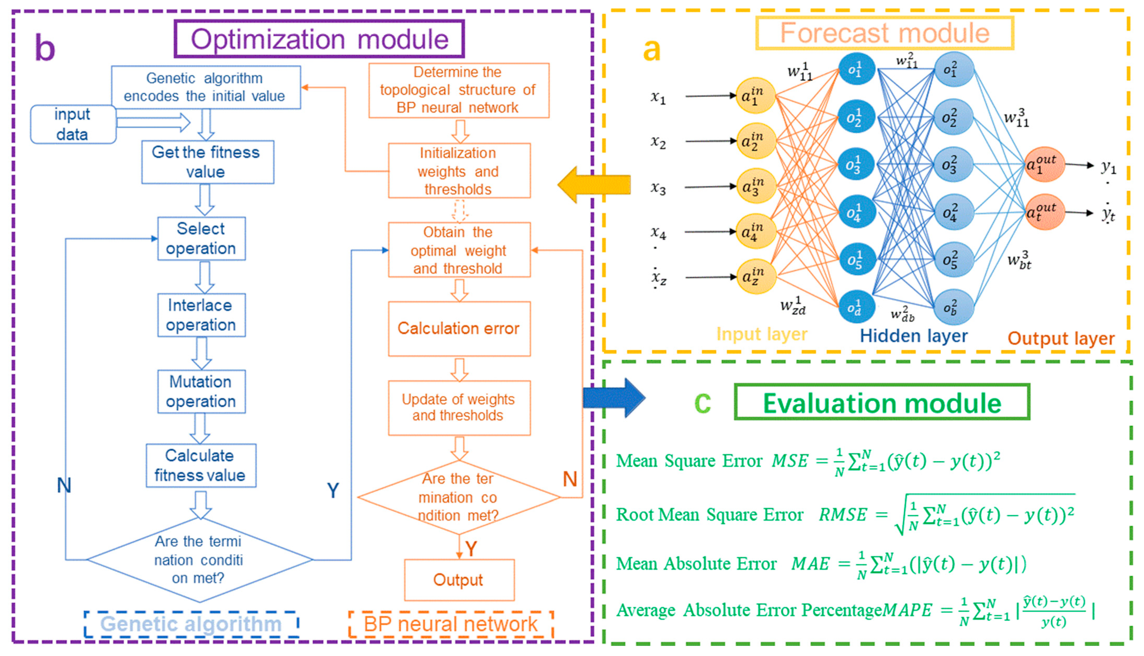
2.1.1. Back-Propagation Neural Network

BP neural network can be analogized as multi-layer perceptron, in which the hidden layer function mostly adopts S-type transfer function, while the output layer neuron mostly adopts linear transfer function. Figure 1a shows the three-layer BP network topology of z × d × b × t, where $\mathrm{z}$ represents the number of input layers, d and b represent the number of two hidden layers, and $\mathrm{t}$ represents the number of output layers. The output calculation process of the BP neural network consists of three steps. First, the input layer is the data of eight meteorological factors obtained through climate monitoring instruments. Second, the obtained output data are compared with the actual data and the error is calculated using the loss function of the evaluation module. Third, the error is propagated backward to find the derivative of the error for each weight in the network and to optimize the model. In a BP artificial neural network, each layer will only transmit data to the next layer. We apply the model to new data to obtain more accurate predictions after repeating the above steps and learning the weights for several times. It can be assumed that the existing sample pairs $\left(\hat{\mathrm{x}},\hat{\mathrm{y}}\right)$ are $\mathrm{x}=\left[{\mathrm{x}}_1,{\mathrm{x}}_2,\dots ,{\mathrm{x}}_{\mathrm{m}}\right]$, $\mathrm{y}=\left[{\mathrm{y}}_1,{\mathrm{y}}_2,\dots ,{\mathrm{y}}_{\mathrm{t}}\right]$, and the hidden layer neurons are $\mathrm{o}=\left[{\mathrm{o}}_1,{\mathrm{o}}_2,\dots ,{\mathrm{o}}_{\mathrm{m}}\right]$. The network weight matrix between the neurons in the input and hidden layers is w¹, and the network weights between the neurons in the hidden and output layers are w³, respectively.

$${\mathrm{w}}^1=\left[\begin{array}{cccc}{\mathrm{w}}_{11}^1& {\mathrm{w}}_{12}^1& \cdots & {\mathrm{w}}_{1\mathrm{d}}^1\\ {\mathrm{w}}_{21}^1& {\mathrm{w}}_{22}^1& \cdots & {\mathrm{w}}_{2\mathrm{d}}^1\\ ⋮& ⋮& \cdots & ⋮\\ {\mathrm{w}}_{\mathrm{m}1}^1& {\mathrm{w}}_{\mathrm{m}2}^1& \cdots & {\mathrm{w}}_{\mathrm{md}}^1\end{array}\right] {\mathrm{w}}^3=\left[\begin{array}{cccc}{\mathrm{w}}_{11}^3& {\mathrm{w}}_{12}^3& \cdots & {\mathrm{w}}_{1\mathrm{t}}^3\\ {\mathrm{w}}_{21}^3& {\mathrm{w}}_{22}^3& \cdots & {\mathrm{w}}_{2\mathrm{t}}^3\\ ⋮& ⋮& \cdots & ⋮\\ {\mathrm{w}}_{\mathrm{b}1}^3& {\mathrm{w}}_{\mathrm{b}2}^3& \cdots & {\mathrm{w}}_{\mathrm{bt}}^3\end{array}\right]$$

(1)

x_i represents the $\mathrm{i}$th input value in a neural network, y is the vector of predicted values,${\mathrm{a}}_{\mathrm{i}}^{\mathrm{l}}$ represents the ith activation of neurons in the ith layer, and ${\mathrm{w}}_{\mathrm{lm}}^{\mathrm{i}}$ represents the connection between the $\mathrm{m}$th unit on the ith layer and the first unit on the (i + 1)th layer.

The threshold values of the hidden layer neuron and the output layer neuron are θ¹ and θ², respectively

$${\mathsf{\theta }}^1=\left[{\mathsf{\theta }}_1^1,{\mathsf{\theta }}_2^1,\dots ,{\mathsf{\theta }}_{\mathrm{l}}^1\right], {\mathsf{\theta }}^2=\left[{\mathsf{\theta }}_1^2,{\mathsf{\theta }}_2^2,\dots ,{\mathsf{\theta }}_{\mathrm{l}}^2\right]$$

(2)

Then the output of hidden layer neurons is

$$\begin{array}{l}{\mathrm{o}}_{\mathrm{j}}={\int }^{}\left({\sum }_1^{\mathrm{m}}{\mathrm{w}}_{\mathrm{ji}}^1{\mathrm{x}}_{\mathrm{i}}-{\mathsf{\theta }}_{\mathrm{j}}^1\right)=\mathrm{f}\left({\mathrm{net}}_{\mathrm{j}}\right),\mathrm{j}=1,2,\cdots ,\mathrm{l}\\ {\mathrm{net}}_{\mathrm{j}}={\sum }_{\mathrm{i}=1}^{\mathrm{m}}{\mathrm{w}}_{\mathrm{ji}}^1-{\mathsf{\theta }}_{\mathrm{j}}^1,\mathrm{j}=1,2,\dots ,\mathrm{l};\mathrm{f}(.)\end{array}$$

(3)

The output of neurons in the output layer is

$$\begin{array}{l}{\mathrm{a}}_{\mathrm{j}}={\int }^{}\left({\sum }_{\mathrm{j}=1}^{\mathrm{l}}{\mathrm{w}}_{\mathrm{kj}}^1{\mathrm{o}}_{\mathrm{i}}-{\mathsf{\theta }}_{\mathrm{k}}^1\right)=\mathrm{g}\left({\mathrm{net}}_{\mathrm{j}}\right),\mathrm{k}=1,2,\cdots ,\mathrm{n}\\ {\mathrm{net}}_{\mathrm{k}}={\sum }_{\mathrm{i}=1}^{\mathrm{m}}{\mathrm{w}}_{\mathrm{kj}}^1-{\mathsf{\theta }}_{\mathrm{k}}^2,\mathrm{k}=1,2,\dots ,\mathrm{n};\mathrm{g}(.)\end{array}$$

(4)

The error between the network output and the expected output is

$$\mathrm{E}=\frac{1}{2}\sum _{\mathrm{k}=1}^{\mathrm{n}}{\left({\mathrm{y}}_{\mathrm{k}}-{\mathrm{z}}_{\mathrm{k}}\right)}^2$$

(5)

2.1.2. BP Neural Network Optimized by GA

GA is an optimization method used to find exact or approximate solutions to optimization problems and search problems applied in many research fields [29]. The BP neural network optimized by GA can effectively avoid the local minimum defects of the original BP neural network, and has the advantages of fast convergence speed and high accuracy [30]. GA is an adaptive heuristic search algorithm that mimics the biological evolutionary mechanism of “survival of the fittest” in nature, and is widely used to solve optimization problems in combination with artificial neural networks [31]. GA is efficient, practical, and robust. GA encodes data into chromosomes, exchanges information in chromosomes through selection, crossover, and iterative variation, and finally finds chromosomes that meet the optimization goal. By selecting, crossing over, and changing populations consisting of a certain number of problem parameters, GA screens out individuals with higher fitness and excludes those with lower fitness [32], and evolves and iterates to find the most satisfactory individual. By coming to optimize the weights and thresholds of the neural network, GA can avoid falling into local optimum and improve the training speed effectively. The algorithm consists of the following eight steps (see Figure 1b).

Step 1: Determine the neural network topology; in this BP neural network model, the input layer is each set of data of eight weather and meteorological factors, and the output layer is the daily average soil moisture, constituting an input layer of eight nodes and an output layer of one node.

Step 2: The initial population is obtained; the population size is set by preprocessing the input data, where each individual contains a real string of ownership values and thresholds for the BP neural network.

Step 3: Setup of fitness function F; The formula is

$$\mathrm{F}={\displaystyle \sum }_{\mathrm{i}=1}^{\mathrm{n}}\left|{\mathrm{f}}_{\mathrm{i}}-\mathrm{f}\left({\mathrm{x}}_{\mathrm{i}}\right)\right|$$

(6)

where f_i is the expected output value and f(x_i) is the actual output value.

Step 4: Selection operations; selection operations are defined as the selection of superior individuals from the original population by a certain probability and the production of the next generation of individuals by reproduction. The probability of individual selection is related to fitness. The higher the fitness, the higher the probability of individual selection. In this paper, roulette is used. The probability of selection is

$${\mathrm{p}}^{\mathrm{i}}=\frac{{\mathrm{F}}_{\mathrm{i}}}{{\sum }_{\mathrm{j}=1}^{\mathrm{N}}{\mathrm{F}}_{\mathrm{j}}}$$

(7)

where F_i is the population fitness value of individual I, and N is the population number.

Step 5: Crossover operation; crossover operation is the random selection of two individuals from a population to transfer the good characteristics of their parents to their offspring through the exchange and combination of their chromosomes to produce new individuals with high adaptability. That is, there are two individuals a_k and a_l which operate at j crossover, as follows

$${\mathrm{a}}_{\mathrm{kj}}={\mathrm{a}}_{\mathrm{kj}}\left(1-\mathrm{b}\right)+{\mathrm{a}}_{\mathrm{lj}}$$

(8)

$${\mathrm{a}}_{\mathrm{lj}}={\mathrm{a}}_{\mathrm{lj}}\left(1-\mathrm{b}\right)+{\mathrm{a}}_{\mathrm{kj}}$$

(9)

where b is a random number between $\left[0,1\right]$.

Step 6: Mutation operations; population diversity can be maintained through population variation. A randomly selected individual from the population and a part of that individual is selected for the mutation operation. in order to produce a better individual. Individual a_i mutates at j, forming a new gene a_ij as follows.

$${\mathrm{a}}_{\mathrm{ij}}=\{\begin{array}{c}{\mathrm{a}}_{\mathrm{ij}}+\left({\mathrm{a}}_{\mathrm{ij}}-{\mathrm{a}}_{\max }\right){\mathrm{r}}_2\left(1-\mathrm{g}/{\mathrm{G}}_{\max }\right), \mathrm{r}\ge 0.5 \\ {\mathrm{a}}_{\mathrm{ij}}+\left({\mathrm{a}}_{\min }-{\mathrm{a}}_{\mathrm{ij}}\right){\mathrm{r}}_2\left(1-\mathrm{g}/{\mathrm{G}}_{\max }\right), \mathrm{r}<0.5\end{array}$$

(10)

where ${\mathrm{a}}_{\max },{\mathrm{a}}_{\min }$ are the upper and lower bounds of a_ij, r₂ is a random number, g is the number of current iterations, and G_max is the maximum number of evolutions.

Step 7: Calculate the fitness of individuals in the newly generated population. If the fitness function meets the requirements or the evolution time reaches the maximum, the evolution is completed, otherwise return to step 4.

Step 8: Through GA optimization, the BP network is given initial weights and thresholds, and the prediction results are obtained after the termination conditions are satisfied.

2.1.3. Error Estimation

The evaluation module assesses the validity and accuracy of the GA-optimized neural network prediction model considering MSE (mean square error), RMSE (root mean square error), MAE (mean absolute error) and MAPE (mean absolute percentage error), respectively (see Figure 1c).

$$\mathrm{MSE}=\frac{1}{\mathrm{N}}{\sum }_{\mathrm{t}=1}^{\mathrm{N}}{(\hat{\mathrm{y}}\left(\mathrm{t}\right)-\mathrm{y}\left(\mathrm{t}\right))}^2$$

(11)

$$\mathrm{RMSE}=\sqrt{\frac{1}{\mathrm{N}}{\sum }_{\mathrm{t}=1}^{\mathrm{N}}{(\hat{\mathrm{y}}\left(\mathrm{t}\right)-\mathrm{y}\left(\mathrm{t}\right))}^2}$$

(12)

$$\mathrm{MAE}=\frac{1}{\mathrm{N}}{\sum }_{\mathrm{t}=1}^{\mathrm{N}}(\left|\hat{\mathrm{y}}\left(\mathrm{t}\right)-\mathrm{y}\left(\mathrm{t}\right)\right|)$$

(13)

$$\mathrm{MAPE}=\frac{1}{\mathrm{N}}{\displaystyle \sum }_{\mathrm{t}=1}^{\mathrm{N}}|\frac{\hat{\mathrm{y}}\left(\mathrm{t}\right)-\mathrm{y}\left(\mathrm{t}\right)}{\mathrm{y}\left(\mathrm{t}\right)}|$$

(14)

where N is the total number of training sets or test sets; $\hat{\mathrm{y}}\left(\mathrm{t}\right)$ and y(t) are the predicted and actual values, respectively.

2.2. GA-BP Soil Moisture Prediction Model

2.2.1. Meteorological Data Monitoring Scheme

A monitoring device and prediction method for vegetation growth environment on slopes in typhoon areas were adopted to address the problems of complicated operation and high cost of monitoring instruments for long-term monitoring of slope environment. By setting up temperature and humidity sensors, soil temperature and humidity, salt integrated sensors, wind speed and direction sensors, rainfall sensing and ware solar radiation sensors, long-term remote monitoring of the slope growth environment is achieved by means of wireless network and cloud platform data transmission. Finally, based on the collected long-term data and the data provided by China Meteorological Network, the time series method and linear regression model are used to make short-term prediction of slope meteorological parameters, so as to obtain the temporal changes of slope meteorological parameters.

The ecological berm meteorological parameter monitoring system consists of temperature and humidity sensors, integrated soil temperature and humidity and salt sensors, wind speed and direction sensors, rainfall sensors, solar radiation sensors, data collectors, wireless communication modules, and a solar power supply system powered by the whole test system. Part of the structure is shown in Figure 2.

The solar radiation sensor, ambient temperature and humidity sensor, and wind speed and direction sensor in the installation were mounted on the top of the slope without vegetation shading, and erected with a triangular bracket at 2 m from the top surface of the slope. The triangular bracket has a horizontal vacuum indicator at the top to ensure the level of the triangular bracket, and then the three corners of the bracket are fixed with expansion screws. The rain sensor is mounted on the top of the slope, unobstructed, and fixed with expansion screws. The integrated soil temperature, moisture, and salinity sensor was installed at the top of the slope by placing the sensor into a hole with a diameter of 50 mm and a depth of 2 m at the top of the slope, bringing the sensor into close contact with the soil, ensuring that the soil fills the sensor, and filling the upper part with soil to prevent water from entering. The wireless communication module and data collector were placed uniformly in the collection box and fixed on a triangular support. The solar power supply system consists of solar photovoltaic panel, battery, and debugger. The solar photovoltaic panel is tilted to the south and placed on a reserved bracket; the battery is placed in a stainless steel box and fixed to the ground with expansion screws. The ambient temperature and humidity sensor, air pressure sensor, solar radiation sensor, rainfall sensor and integrated soil temperature, humidity and salt sensor are connected to the collector through the data line, and the collected data enter the data collector through the data line. The data collector uploads the collected data to the cloud platform server in real time through the wireless communication module, and the client computer can view and download the test data by accessing the cloud, thus realizing the long-term monitoring of the vegetation growth environment on the slope.

2.2.2. Influencing Factors of Soil Moisture

Soil moisture of ecological berm is closely related to local meteorological factors, and soil moisture is influenced not only by its own hydrological factors, but also by surrounding meteorological factors. The movement of the atmospheric system is a highly unified process of determinism and stochasticity. From a macroscopic point of view, the uncertainty of soil moisture variation is mainly determined by the influence of preexisting meteorological conditions. Climate is the main factor that determines the distribution of soil moisture on earth, while the uncertainty of soil moisture mainly comes from the stochastic nature of atmospheric factors. Therefore, meteorological factors can be used to predict soil moisture. In this paper, nine meteorological factors are obtained, namely, daily maximum ambient temperature (X₁), daily minimum ambient temperature (X₂), daily average temperature (X₃), daily average ambient humidity (X₄), daily average dew point temperature (X₅), daily average wind speed (X₆), daily average rainfall (X₇), daily total solar radiation (X₈), and daily average soil temperature (X₉). The Pearson correlation coefficient and Spearman correlation coefficient are shown in Figure 3.

In general, the correlation strength of the variables can be judged by the following range of values, with correlation coefficients in the range of 0.8–1.0 for very strong correlation, 0.6–0.8 for strong correlation, 0.4–0.6 for moderate correlation, 0.2–0.4 for weak correlation, and 0.0–0.2 for very weak or no correlation. The correlation was based on the Pearson correlation coefficient and Spearman correlation coefficient between meteorological factors and soil moisture, and it was found that (Y) was very strongly correlated with (X₂), (X₅), and (X₉), strongly correlated with (X₁) and (X₃), and moderately correlated with (X₄) and (X₈). The Pearson correlation coefficient between (Y) and (X₇) shows a strong correlation, and the Spearman correlation coefficient turns out to be weakly correlated. (Y) showed a very weak or no correlation with (X₆), so this factor was excluded (see Figure 3).

Atmospheric temperature and soil temperature exchange heat directly due to the presence of temperature differences, so changes in temperature can affect changes in soil moisture. Wind can contribute to the decrease of soil moisture by promoting the evaporation of water to absorb heat, showing a negative correlation. The relative humidity of air can prevent a certain amount of solar radiation from being absorbed by the ground and can also prevent the escape of long-wave radiation from the ground. Soil moisture has different lag times for each meteorological factor, with temperature and wind speed having the most rapid effect on soil temperature, followed by total solar radiation, and relative humidity the slowest. Considering that the lag time of soil moisture to total solar radiation and ambient humidity is more obvious, the lag is considered for prediction. After considering their lags, the correlation coefficients are significantly improved, as shown in

Table 2. Comparison Table of Hysteresis of X₄, X₈, and Y.

	Pearson		Spearman
	Original	Consider Lag	Original	Consider Lag
X4	0.472	0.521	0.468	0.543
X8	0.443	0.471	0.475	0.546

.

Considering the discrete nature of field monitoring results due to small samples and many factors, a neural network algorithm optimized by GA was used. Among 100 days of monitoring data, the meteorological data of the first 90 days were selected as the training samples and the data of the last 10 days as the prediction samples and the GA-BP regression prediction model was programmed by MATLAB language. Experimental data for meteorological factors and soil moisture are shown in

Table A1. Experimental data on meteorological factors and soil moisture.

NO	X1	X2	X3	X4	X6	X7	X8	X9	Y
1	35.2	23.0	30.3	76.4	24.7	0.0	16.507	32.8	89.8
2	35.3	23.5	29.0	87.5	24.2	25.2	25.182	32.6	97.3
3	35.5	23.8	29.5	77.4	23.8	0.0	23.640	32.9	88.4
4	35.2	24.0	29.8	73.1	23.9	0.0	24.608	33.2	82.7
5	35.2	23.1	29.2	72.0	23.4	0.0	24.388	33.4	77.5
6	34.6	24.0	29.2	72.6	23.7	0.0	20.348	33.8	72.2
7	33.6	23.5	28.3	73.5	23.0	0.0	19.015	33.7	68.0
8	31.4	22.8	25.4	74.2	23.1	0.0	17.639	33.3	70.2
9	31.4	22.9	25.5	88.3	23.9	20.4	16.773	32.5	85.9
10	32.6	23.8	27.7	91.8	24.4	13.8	21.756	32.8	90.7
11	33.4	23.7	28.3	83.7	23.3	0.6	23.803	32.7	86.1
12	32.4	23.0	27.9	75.8	23.1	0.0	21.893	32.9	80.2
13	32.0	25.0	27.8	76.6	24.8	0.0	14.121	33.0	77.3
14	28.4	25.1	26.3	84.0	24.2	3.8	5.473	32.1	80.1
15	26.6	24.6	25.4	88.2	24.7	45.2	2.559	30.8	80.4
16	35.4	24.3	29.1	96.0	23.9	115.0	23.970	32.3	95.8
17	34.6	24.2	28.5	76.4	22.9	0.2	20.727	32.5	92.8
18	32.8	24.1	26.7	74.1	24.1	0.0	15.309	32.5	90.3
19	33.9	23.1	28.1	86.0	24.2	2.4	19.501	32.8	86.9
20	34.6	24.4	28.4	80.5	24.1	0.0	16.651	32.9	81.0
21	34.9	24.0	28.6	79.2	23.7	0.0	18.871	33.0	77.2
22	35.4	22.8	28.1	77.4	21.5	0.0	24.005	33.2	73.5
23	34.4	21.1	26.8	71.2	22.0	0.0	21.653	33.2	75.0
24	33.5	21.6	26.0	77.7	22.4	16.2	23.018	33.0	86.3
25	34.9	24.6	28.9	79.5	24.4	1.6	23.473	33.8	69.5
26	32.3	23.9	27.3	78.5	24.5	0.0	17.620	33.7	68.6
27	29.8	25.7	27.1	85.2	25.2	4.4	9.818	33.0	72.0
28	34.5	24.6	28.8	89.8	24.9	5.4	19.222	33.1	64.4
29	35.5	24.4	29.3	81.2	25.1	0.0	24.055	33.5	64.6
30	35.3	25.2	29.5	79.8	25.3	0.0	20.844	33.9	63.1
31	29.2	21.6	24.2	79.5	20.7	0.4	12.676	33.4	61.5
32	25.6	18.4	21.5	81.5	19.7	0.0	8.594	31.3	75.8
33	24.0	20.0	22.2	90.0	21.1	48.6	3.131	30.2	80.5
34	25.5	21.3	22.9	93.7	21.0	1.4	5.650	30.0	82.7
35	25.6	21.2	22.3	89.0	21.9	3.2	5.982	29.8	96.5
36	28.1	20.7	24.4	97.2	22.1	33.8	14.858	30.5	89.3
37	29.3	23.3	25.0	88.1	23.5	0.0	10.248	30.7	92.5
38	30.5	22.6	25.1	91.6	23.2	4.8	16.909	31.0	93.0
39	28.3	22.8	24.8	90.2	22.2	3.8	10.742	30.7	90.6
40	31.3	21.7	25.1	86.5	22.0	4.2	19.939	30.5	86.0
41	31.3	18.9	25.0	83.5	19.9	0.0	21.053	30.8	75.9
42	21.2	18.1	19.8	75.4	16.1	0.0	4.049	27.6	52.8
43	27.0	16.0	21.2	79.8	13.8	2.2	19.345	28.0	49.8
44	27.8	13.5	20.3	65.3	11.8	0.0	19.987	28.0	47.4
45	28.8	13.7	20.3	62.7	12.4	0.0	19.160	28.0	47.1
46	28.5	14.5	21.3	64.5	14.8	0.0	18.083	28.1	46.7
47	28.9	15.5	22.3	69.1	15.4	0.0	18.158	28.7	46.5
48	28.8	19.6	23.6	69.0	17.3	0.0	12.896	19.4	46.2
49	30.4	17.7	23.5	69.8	17.2	0.0	17.294	19.5	45.9
50	28.1	19.6	22.9	70.8	18.6	0.0	11.017	29.4	45.5
51	23.3	21.1	21.8	78.6	20.1	0.0	2.601	28.6	68.0
52	29.4	21.0	25.0	90.0	19.8	91.0	13.533	28.5	76.8
53	30.8	19.3	24.5	74.0	20.6	0.0	16.941	28.9	73.4
54	30.2	21.6	25.1	80.6	22.1	0.0	14.508	29.3	70.3
55	28.1	21.5	24.1	84.4	20.9	0.0	6.346	29.4	68.0
56	22.5	16.7	19.3	83.4	16.2	0.0	5.624	27.1	58.8
57	29.1	19.2	22.3	82.6	18.4	0.0	14.840	27.7	58.7
58	30.2	19.8	24.4	79.4	19.9	0.0	13.091	28.5	57.7
59	23.3	20.0	21.7	77.3	18.6	0.0	3.326	28.4	56.3
60	24.9	19.4	21.4	82.7	17.2	0.0	7.914	27.9	55.1
61	23.4	18.5	19.8	77.9	16.8	0.0	5.089	27.6	54.2
62	21.4	12.6	17.7	83.1	11.6	0.0	19.891	26.2	49.0
63	22.0	15.6	18.3	68.1	13.3	0.0	9.786	26.1	48.4
64	21.3	13.3	17.2	73.3	11.8	0.0	9.410	25.9	48.0
65	22.6	11.7	16.7	71.1	10.6	0.0	15.415	25.3	47.7
66	23.1	11.0	16.6	70.0	11.4	0.0	14.746	25.0	46.9
67	23.5	10.9	16.6	73.6	10.8	0.0	15.462	24.8	46.6
68	24.2	11.5	17.4	72.3	11.8	0.0	15.219	24.8	46.4
69	23.8	15.8	19.1	72.5	13.2	0.0	11.752	25.3	46.2
70	23.5	14.3	18.4	70.5	12.8	0.0	14.464	25.3	46.0
71	23.7	12.5	18.0	72.1	11.1	0.0	12.012	24.9	45.5
72	19.5	14.6	17.0	67.2	13.6	0.0	4.576	25.1	45.9
73	14.9	13.8	14.3	80.7	13.9	1.0	1.382	24.3	57.5
74	16.0	13.6	14.7	97.7	14.4	10.8	2.240	23.8	64.7
75	22.3	11.0	15.8	98.0	1.6	6.2	13.562	23.7	60.8
76	22.0	8.3	14.2	79.0	7.3	0.2	14.117	22.9	55.5
77	23.7	8.7	14.9	68.2	8.7	0.0	14.125	22.5	52.0
78	22.6	9.8	15.4	70.1	10.3	0.0	13.488	22.4	49.5
79	22.8	11.1	16.3	74.5	12.5	0.0	12.627	22.5	48.5
80	18.3	13.3	15.2	80.2	13.9	0.0	3.378	22.7	48.6
81	20.9	12.1	16.1	91.7	12.2	0.0	10.886	22.8	48.3
82	20.0	10.5	15.1	79.3	8.7	0.2	12.490	22.5	47.3
83	16.8	9.4	12.1	69.1	10.1	0.0	13.420	21.8	48.1
84	17.5	14.1	15.2	87.5	13.8	1.2	2.535	22.7	53.1
85	18.0	9.5	14.8	92.0	9.6	1.6	9.678	22.5	48.2
86	18.6	7.6	12.1	72.3	6.2	0.0	12.872	21.3	46.6
87	21.6	6.0	12.6	71.0	6.3	0.0	12.575	20.5	46.5
88	22.5	8.6	14.7	69.0	7.2	0.0	12.613	20.7	45.3
89	18.7	11.7	14.8	65.2	10.5	0.0	4.520	21.1	45.2
90	20.0	12.8	16.8	76.0	11.3	0.0	7.710	21.9	45.4
91	15.7	0.4	7.1	61.0	0.1	0.0	5.700	14.7	41.6
92	18.0	3.4	9.4	64.9	2.7	0.0	10.387	15.5	41.6
93	18.1	3.9	10.3	66.0	1.3	0.0	10.242	15.6	41.5
94	14.7	2.7	8.6	56.4	1.7	0.0	10.199	15.6	41.2
95	17.0	2.9	9.0	63.9	4.7	0.0	10.142	15.6	41.2
96	18.7	5.5	11.1	76.2	5.7	0.0	9.644	16.1	41.3
97	19.5	5.9	12.3	72.0	8.1	0.0	9.544	16.6	41.4
98	23.4	11.3	16.6	77.5	12.6	0.0	10.297	18.2	41.9
99	24.7	11.2	16.4	78.6	12.7	0.0	9.318	19.3	42.1
100	11.1	8.3	9.5	80.2	6.9	0.0	1.494	18.7	41.4

.

3. Results

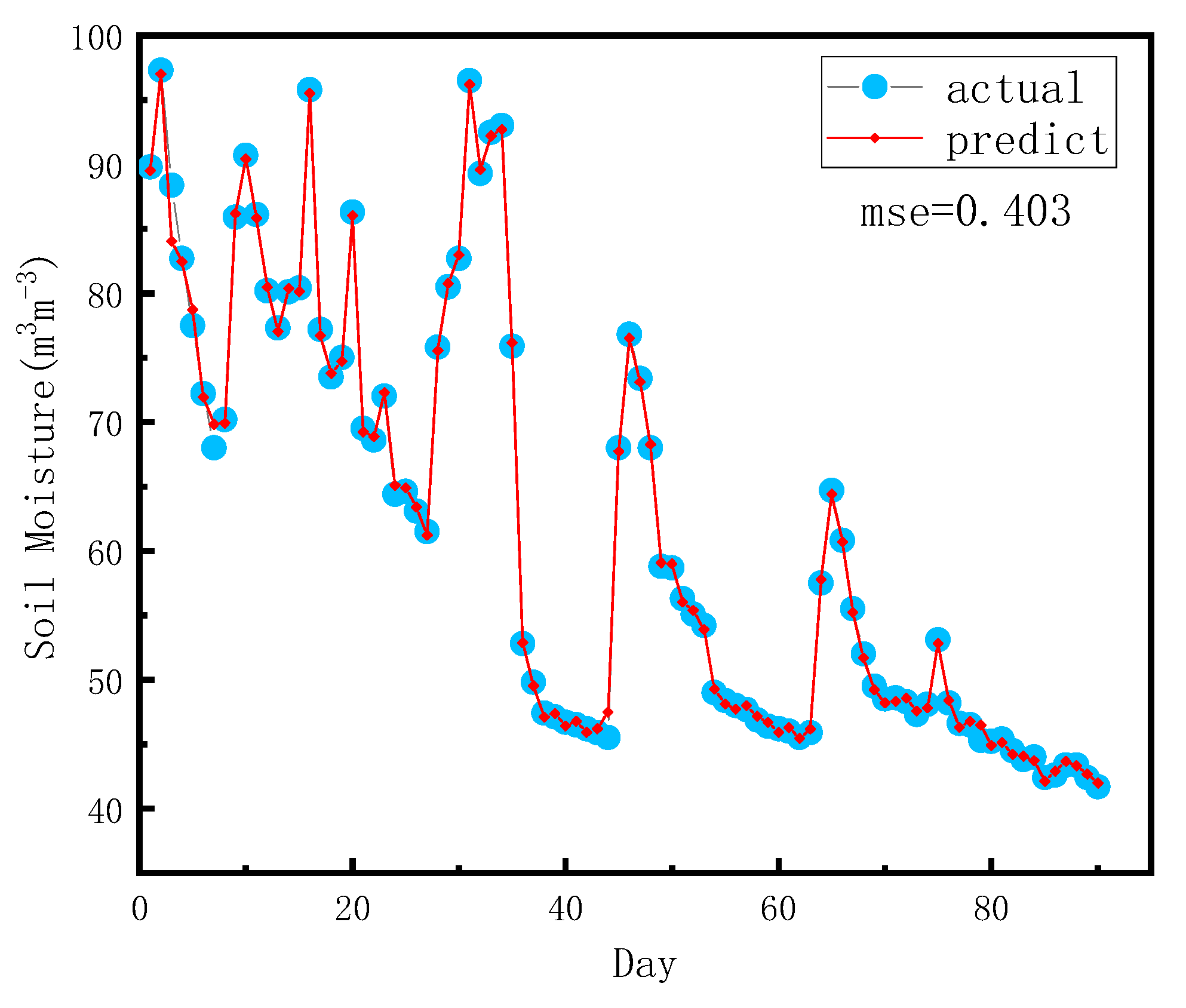
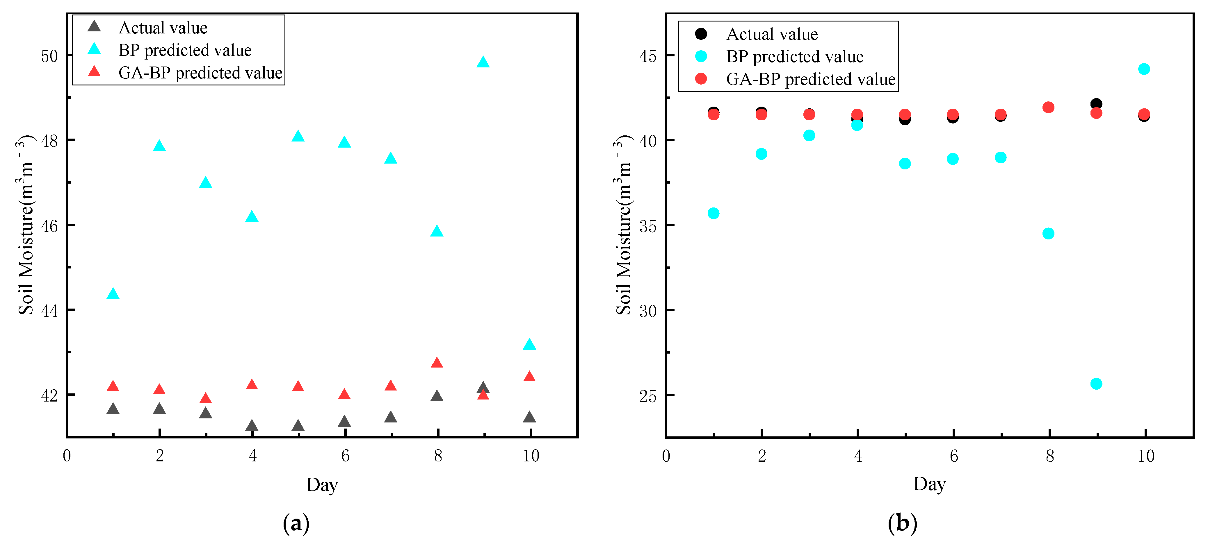
3.1. Comparison of Model Prediction

A GA-BP regression prediction model was developed using 100 days of data obtained through a meteorological monitoring system as the experimental object. Eight meteorological factors were used as the input layer and soil moisture was used as the output layer. Among them, the first 90 days of monitoring data were used as the training set and 10 days of data were used as the test set, and the soil moisture of the ecological berm was simulated and predicted by neural network. In this prediction model, the crossover probability was 0.8, the variance probability was 0.05, the initial population size was 100, and the maximum evolutionary generation was 100. Prediction simulation experiments were conducted using Matlab software and the prediction results were compared. The results of the training set considering the lag are shown in Figure 4.

After running the program, the MAE, MSE, RMSE, and MAPE can be obtained by the above equations, the BP neural network prediction model is compared with the GA-optimized neural network prediction model, the prediction results of the original data are compared with the prediction results considering the lag, and the re-derived results are shown in Figure 5 and

Table 3. Error analysis of BP and GA-BP.

		MAE	MSE	RMSE	MAPE
Original	BP	5.221	30.549	5.527	12.574%.
	GA-BP	0.661	0.505	0.711	1.595%.
Consider lag	BP	4.424	39.792	6.308	10.592%.
	GA-BP	0.171	0.0516	0.227	0.412%.

.

The MSE of the training set with lags is 0.403. By observing (a) and (b) in Figure 5, it is easy to find that the accuracy of the BP prediction model with lags is lower than that without lags, while the accuracy of the GA-BP prediction model with lags is higher than that without lags, and the accuracy of the GA-BP prediction model with lags is better. The GA-BP prediction model is significantly better than the BP prediction model. Through Table 3, comparing the original data and the prediction model considering lags, it can be seen that the GA-BP neural network prediction model has an MSE of 0.505 and a MAPE of 1.595% for the original data. The MSE and MAPE of the GA-BP prediction model considering lags were 0.0516 and 0.412%, respectively. The MSE of the BP prediction model was 39.7918 and the mean absolute error MAPE was 10.592%, which was larger for the prediction of soil moisture. The GA-BP prediction model considering hysteresis has good prediction effect, and the error is controlled around 0.01, which can predict soil moisture more accurately.

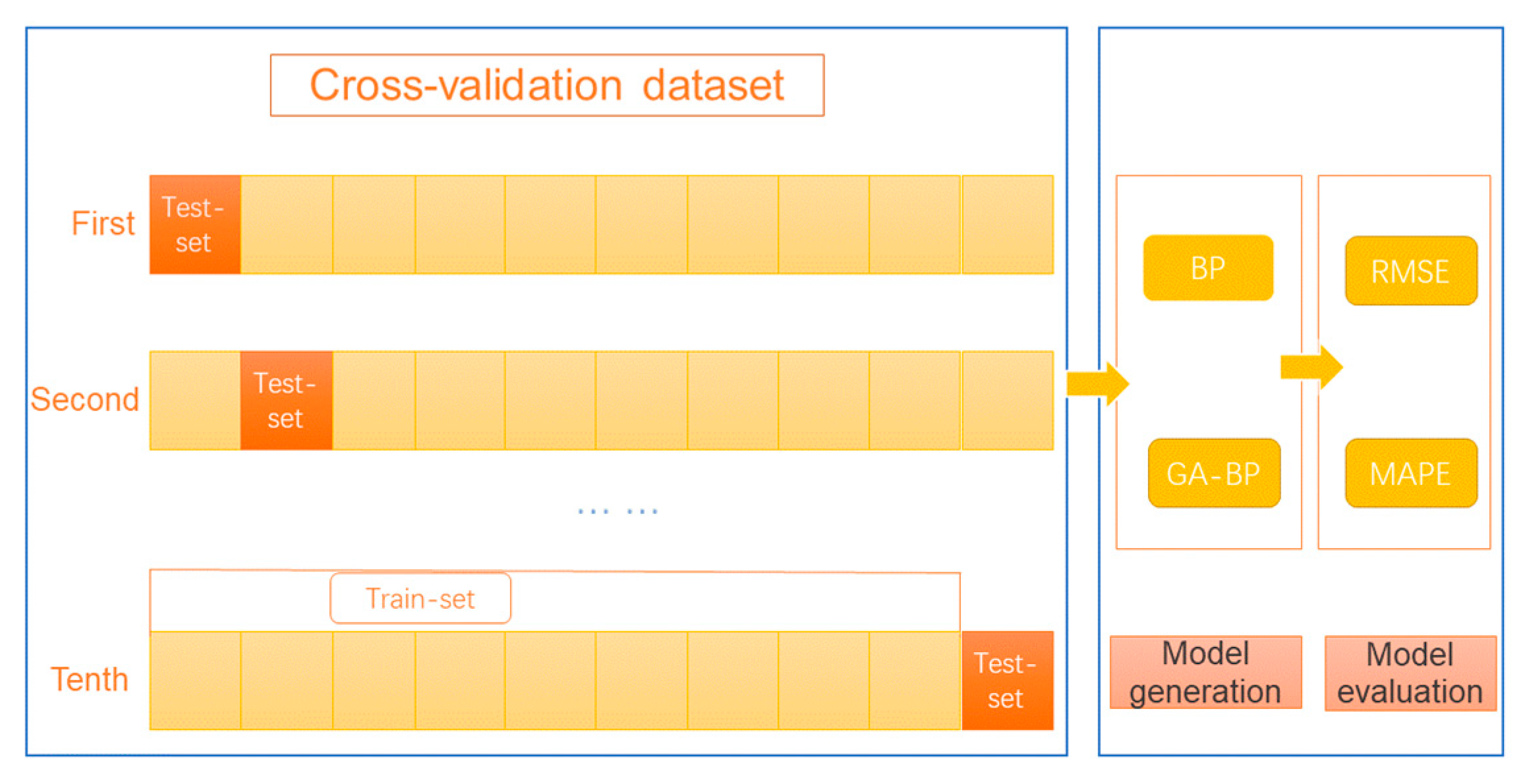
3.2. Prediction Model Evaluation

The cross-validation method was selected to evaluate the soil moisture prediction model. The cross-validation method is a method that eliminates the bias caused by random sampling during sample training and is a method that directly estimates the generalization error without any preconditions. Cross-validation refers to dividing the original data into a training set and a test set according to the prediction settings of the neural network. The training set is used to train the model and the test sample is used to validate the trained model to evaluate the prediction accuracy of the model. We use the V-fold cross-validation method to evaluate the prediction model. The V-fold cross-validation method refers to dividing the data into V parts, selecting one of them as the test set and V-1 part as the test set, repeating v times, and finally analyzing the average error of v times as the performance index for model evaluation. In this paper, 100 sets of data are divided into 10 parts in chronological order, and the GA-BP prediction model considering lag is evaluated by the V-fold cross-validation method, as shown in Figure 6.

From

Table 4. Statistics of cross-validation evaluation index parameters.

NO	RMSE		MAPE
	BP	GA-BP	BP	GA-BP
1	6.308	0.227	10.592%	0.412%.
2	1.739	0.555	3.247%	1.283%.
3	9.020	0.424	19.663%	0.825%.
4	2.445	0.798	3.556%	1.824%.
5	4.264	0.811	9.336%	1.698%.
6	4.006	0.287	7.603%	0.573%.
7	2.167	0.480	4.268%	1.065%.
8	6.895	0.685	13.888%	1.516%.
9	6.586	0.662	10.020%	1.353%.
10	5.026	0.466	10.986%	0.975%.
Average value	4.845	0.540	9.316%	1.152%.

, it can be seen that the average RMSE and MAPE of the BP neural network prediction model are 4.845 and 9.316%, respectively, while the average RMSE and MAPE of the GA-BP neural network prediction model are 0.540 and 1.152%, respectively. After cross-validation, it is obvious that the prediction results of BP neural network fluctuate a lot, while the prediction results of GA-BP neural network are relatively stable. Ten experiments show that the accuracy of its model is greatly improved compared with BP neural network. It is not reliable to evaluate the accuracy of the model by the accuracy of one prediction, and there is an element of random error. After cross-validation, it is more reasonable to use the average of RMSE and MAPE as the evaluation criteria of the model.

4. Discussion and Outlook

In this study, we investigated the meteorological factor monitoring and soil moisture prediction methods for high and steep slopes, and proposed a machine learning-based soil moisture prediction method. The correlation between meteorological factors and soil moisture was obtained by analyzing meteorological factors and soil moisture using MATLAB software, and a soil moisture prediction method of BP neural network optimized by genetic algorithm considering hysteresis was established. The results show that the prediction results obtained by the method have a small error with the actual results and a high accuracy.

We compared two prediction methods, BP neural network and GA-BP neural network, to determine the accuracy of soil moisture prediction. BP neural network has the problem of falling into local optimum, so the accuracy of this prediction method is low. For the proposed GA-BP neural network prediction method, the advantage of this method is that it can optimize the defects of the BP neural network itself, and the accuracy of the prediction results is significantly improved.

At present, the research on predicting soil moisture through the correlation between meteorological factors and soil moisture is still in its initial stage. The factors affecting soil moisture are many and complex, and the prediction methods still need to be improved continuously. In this paper, we consider the lag of total solar radiation and relative humidity on soil moisture, but meteorological factors such as sunshine duration and atmospheric pressure also have important effects on the variation of soil moisture. Therefore, in order to predict soil moisture more scientifically and accurately, a more comprehensive and in-depth study of the correlation between soil moisture and meteorological factors is needed. Soil moisture varies with soil depth, so further re-examination of soil moisture variation at different soil depths is needed.

References

1. Huang, S.; Ding, J.; Zou, J.; Liu, B.; Zhang, J.; Chen, W. Soil Moisture Retrival Based on Sentinel-1 Imagery under Sparse Vegetation Coverage. Sensors 2019, 19, 589. [Google Scholar] [CrossRef] [PubMed] [Green Version]
2. Li, X.; Huo, Z.; Xu, B. Optimal Allocation Method of Irrigation Water from River and Lake by Considering the Field Water Cycle Process. Water 2017, 9, 911. [Google Scholar] [CrossRef] [Green Version]
3. Liao, R.; Yang, P.; Wang, Z.; Wu, W.; Ren, S. Development of a Soil Water Movement Model for the Superabsorbent Polymer Application. Soil Sci. Soc. Am. J. 2018, 82, 436–446. [Google Scholar] [CrossRef]
4. Liang, Y.; Kang, S.; Zhang, C. The Effects of Soil Moisture and Nutrients on Cropland Productivity in the Highland Area of the Loess Plateau. Aciar. Gov. Au. 2002, 14, 187–194. [Google Scholar]
5. Ngo, H.T.T.; Cavagnaro, T.R. Interactive effects of compost and pre-planting soil moisture on plant biomass, nutrition and formation of mycorrhizas: A context dependent response. Sci. Rep. 2018, 8, 1–9. [Google Scholar] [CrossRef] [Green Version]
6. Chang, J.H. Climate and Agriculture: An Ecological Survey, 1st ed.; Routledge: New York, NY, USA, 1968; pp. 286–287. [Google Scholar]
7. Rockström, J.; Williams, J.; Daily, G.; Noble, A.; Matthews, N.; Gordon, L.; Wetterstrand, H.; Declerck, F.; Shah, M.; Steduto, P.; et al. Sustainable intensification of agriculture for human prosperity and global sustainability. Ambio 2016, 46, 4–17. [Google Scholar] [CrossRef] [Green Version]
8. Feng, H. Individual contributions of climate and vegetation change to soil moisture trends across multiple spatial scales. Sci. Rep. 2016, 6, 32782. [Google Scholar] [CrossRef] [Green Version]
9. Martínez-Fernández, J.; González-Zamora, A.; Sánchez, N.; Gumuzzio, A.; Herrero-Jiménez, C. Satellite soil moisture for agricultural drought monitoring: Assessment of the SMOS derived Soil Water Deficit Index. Remote Sens. Environ. 2016, 177, 277–286. [Google Scholar] [CrossRef]
10. Chukalla, A.D.; Krol, M.S.; Hoekstra, A.Y. Green and blue water footprint reduction in irrigated agriculture: Effect of irrigation techniques, irrigation strategies and mulching. Hydrol. Earth Syst. Sci. 2015, 19, 4877–4891. [Google Scholar] [CrossRef] [Green Version]
11. Feki, M.; Ravazzani, G.; Ceppi, A.; Milleo, G.; Mancini, M. Impact of Infiltration Process Modeling on Soil Water Content Simulations for Irrigation Management. Water 2018, 10, 850. [Google Scholar] [CrossRef] [Green Version]
12. Chauhan, Y.S.; Ryan, M.; Chandra, S.; Sadras, V.O. Accounting for soil moisture improves prediction of flowering time in chickpea and wheat. Sci. Rep. 2019, 9, 7510. [Google Scholar] [CrossRef] [PubMed]
13. Cai, Y.; Zheng, W.; Zhang, X.; Zhangzhong, L.; Xue, X. Research on soil moisture prediction model based on deep learning. PLoS ONE 2019, 14, e0214508. [Google Scholar] [CrossRef] [PubMed]
14. Scott, C.A.; Bastiaanssen, W.G.M.; Ahmad, M.-U. Mapping Root Zone Soil Moisture Using Remotely Sensed Optical Imagery. J. Irrig. Drain. Eng. 2003, 129, 326–335. [Google Scholar] [CrossRef] [Green Version]
15. Notarnicola, C.; Angiulli, M.; Posa, F. Soil moisture retrieval from remotely sensed data: Neural network approach versus Bayesian method. IEEE Trans. Geosci. Remote. Sens. 2008, 46, 547–557. [Google Scholar] [CrossRef]
16. Pandey, D.K.; Maity, S.; Bhattacharya, B.; Misra, A. Model-based surface soil moisture (SSM) retrieval algorithm using multi-temporal RISAT-1 C-band SAR data. Land Surf. Cryosphere Remote Sens. III 2016, 9877, 98770X. [Google Scholar] [CrossRef]
17. Then, Y.L.; You, K.Y.; Dimon, M.N.; Lee, C.Y. A modified microstrip ring resonator sensor with lumped element modeling for soil moisture and dielectric predictions measurement. Measurement 2016, 94, 119–125. [Google Scholar] [CrossRef]
18. Holland, J.E.; Biswas, A. Predicting the mobile water content of vineyard soils in New South Wales, Australia. Agric. Water Manag. 2015, 148, 34–42. [Google Scholar] [CrossRef]
19. Liu, M.; He, Z.-M. Research and Prediction of Yellow Soil Moisture Content in Guizhou Province Based on ARIMA Model. Adv. Mater. Res. 2013, 690–693, 3076–3081. [Google Scholar] [CrossRef]
20. Carlson, T. An Overview of the “Triangle Method” for Estimating Surface Evapotranspiration and Soil Moisture from Satellite Imagery. Sensors 2007, 7, 1612–1629. [Google Scholar] [CrossRef] [Green Version]
21. Gill, M.K.; Asefa, T.; Kemblowski, M.W.; McKee, M. SOIL MOISTURE PREDICTION USING SUPPORT VECTOR MACHINES. J. Am. Water Resour. Assoc. 2006, 42, 1033–1046. [Google Scholar] [CrossRef]
22. Zhu, Q.; Wang, Y.; Luo, Y. Improvement of multi-layer soil moisture prediction using support vector machines and ensemble Kalman filter coupled with remote sensing soil moisture datasets over an agriculture dominant basin in China. Hydrol. Process. 2021, 35, e14154. [Google Scholar] [CrossRef]
23. Ji, R.H.; Zhang, S.L.; Zheng, L.H.; Liu, Q.X.; Iftikhar, A.S. Prediction of soil moisture with complex-valued neural network. In Proceedings of the 2007 29th Chinese Control and Decision Conference (CCDC 2017), Chongqing, China, 28–30 May 2017. [Google Scholar]
24. Yang, Z.; Zhao, J.; Liu, J.; Wen, Y.; Wang, Y. Soil Moisture Retrieval Using Microwave Remote Sensing Data and a Deep Belief Network in the Naqu Region of the Tibetan Plateau. Sustainability 2021, 13, 12635. [Google Scholar] [CrossRef]
25. Xu, J.; Zhao, J.; Zhang, W.; Hu, Z.; Zheng, Z. Mid-short-term daily runoff forecasting by ANNs and multiple process-based hy-drological models. In Proceedings of the 2009 IEEE Youth Conference on Information, Computing and Telecommunication, Beijing, China, 20–21 September 2009. [Google Scholar]
26. Xu, J.; Zhu, X.; Zhang, W.; Xu, X.; Xian, J. Daily streamflow forecasting by Artificial Neural Network in a large-scale basin. In Proceedings of the 2009 IEEE Youth Conference on Information, Computing and Telecommunication, Beijing, China, 20–21 September 2009. [Google Scholar]
27. Allen, D.M. The Relationship Between Variable Selection and Data Agumentation and a Method for Prediction. Technometrics 1974, 16, 125–127. [Google Scholar] [CrossRef]
28. Geisser, S. The Predictive Sample Reuse Method with Applications. J. Am. Stat. Assoc. 1975, 70, 320–328. [Google Scholar] [CrossRef]
29. Kurban, T.; Beşdok, E. A Comparison of RBF Neural Network Training Algorithms for Inertial Sensor Based Terrain Classification. Sensors 2009, 9, 6312–6329. [Google Scholar] [CrossRef] [Green Version]
30. Qi, A. Research on Prediction Model of Improved BP Neural Network Optimized by Genetic Algorithm. Adv. Eng. Res. 2018, 150, 764–767. [Google Scholar] [CrossRef] [Green Version]
31. Witten, I.H.; Frank, E.; Hall, M.A.; Christopher, J.P. Data Mining: Practical Machine Learning Tools and Techniques, 4th ed.; Elsevier: Amsterdam, The Netherlands, 2017; pp. 67–89. [Google Scholar]
32. Lee, H.W.; Azid, I.H.A. Neuro-Genetic Optimization of the Diffuser Elements for Applications in a Valveless Diaphragm Micropumps System. Sensors 2009, 9, 7481–7497. [Google Scholar] [CrossRef]
Figure 1. Overall prediction module; neural network prediction structure module: (a) neural network prediction model; (b) optimization module—optimized by genetic algorithm; and (c) error evaluation module.
Sustainability 14 01386 g001
Figure 2. Environmental monitoring system: (a) schematic diagram; (b) physical diagram.
Sustainability 14 01386 g002
Figure 3. Correlation analysis of soil moisture and meteorological factors: (a) Spearman correlation coefficient; (b) Pearson correlation coefficient. The red word means that the correlation between wind speed (X6) and soil moisture is extremely weak. Based on this correlation, wind speed is excluded from soil moisture prediction.
Sustainability 14 01386 g003
Figure 4. Training set prediction considering lag.
Sustainability 14 01386 g004
Figure 5. Soil moisture prediction analysis: (a) BP and GA-BP prediction analysis of original data; (b) BP and GA-BP prediction analysis considering lags.
Sustainability 14 01386 g005
Figure 6. Cross-validation evaluation of predictive models.
Sustainability 14 01386 g006