


Spatial Validation of Agent-Based Models
1
School of Social Science, Policy & Evaluation, Claremont Graduate University, Claremont, CA 91711, USA
2
Department of Public Administration, Portland State University, Portland, OR 97207-0751, USA
*
Author to whom correspondence should be addressed.
Sustainability 2022, 14(24), 16623; https://doi.org/10.3390/su142416623
Submission received: 20 October 2022
/
Revised: 29 November 2022
/
Accepted: 30 November 2022
/
Published: 12 December 2022
(This article belongs to the Topic Advances in Sustainable Communities, Neighborhoods and 15-Minute Cities-Theory, Methods and Techniques)
Abstract
:This paper adapts an existing techno–social agent-based model (ABM) in order to develop a new framework for spatially validating ABMs. The ABM simulates citizen opposition to locally unwanted land uses, using historical data from an energy infrastructure siting process in Southern California. Spatial theory, as well as the model’s design, suggest that adequate validation requires multiple tests rather than relying solely on a single test-statistic. A pattern-oriented modeling approach was employed that first mapped real and simulated citizen comments across the US Census tract. The suite of spatial tests included Global Moran’s I, complemented with bivariate correlations, as well as the local indicators of spatial association (LISA) test. The global tests showed the model explained up to 65% of the variation in the historical data for US Census tract-level citizen comments on a locally unwanted land use. These global tests were also found helpful to inform the model’s calibration for the current application. The LISA results were even stronger, showing that the model predicted citizen comment clustering correctly in five of six Census tracts. It slightly over predicted comments further away from the land use. The LISA results and pattern-oriented modeling validation techniques identified theoretical factors to improve the modeling specification in future applications. The combined suite of validation techniques helped improve confidence in the model’s predictions.
1. Introduction
The purpose of this paper is to outline a robust process of validating a spatially-explicit agent-based model (ABM) of locally unwanted land uses. ABMs allow for studying complex systems behavior and networks by using a set of fixed assumptions and then using an experimental method to generate data which can then be examined inductively [1]. In general, validating the predictions of ABMs is important because in many cases the ABM model is representing a complex social–political–ecological system whose key drivers are not well understood, or there is significant disagreement about the relative importance of those drivers. These drivers can include initial conditions, temporal effects, interaction structures, measurement error, micro-macro feedbacks, and other possible variables. This is a type of “epistemic” uncertainty [2] that ABMs attempt to shed light on using a parsimonious representation of the true system. Fortunately, the suitability of the model’s design and assumptions can then be tested by comparing the modeling predictions to historical outcomes.
The ABM used in this paper, the Redondo Beach energy project (RBEP) model, is an application of the sustainable energy modeling program (SEMPro) [3]. RBEP simulates and predicts citizen opposition to natural gas electricity projects and generates output with details on the number of comments sent in opposition to the project, as well as the location of the senders of these comments. RBEP and SEMPro are a part of a new class of techno–social [4] and complex adaptive systems’ models [3,5]. The models simulate the synergistic effects between human behavior, institutions, engineered physical components, and geophysical elements. The RBEP model is an ABM model with integrated geographic information system information (ABM-GIS). ABM-GIS models can offer significant advantages over traditional ABMs.
The first advantage of an ABM-GIS is that the GIS model allows for accurate validation of the model against “historical outcomes, demographic information, and other empirical data” [6]. RBEP includes spatially explicit analysis through the integration of US Census block group-level geographies data (shape files). This allows for the representation of spatial aspects in the analysis by replicating the geographic structure of the local community in the RBEP model.
In addition to the integration of GIS, the next advantage of ABM-GIS models is that they can use additional data, such as survey or US Census data, as a basis for determining the agents’ attributes. This makes the agents in the model more closely resemble the real people they are simulating. In other words, qualitative data on the citizens in a particular community informs the assumptions and equations of the modeling simulations (and quantitative analysis). RBEP includes Census tract-level attributes on median educational attainment, household income, and population density.
Having connected all these geographies and their attributes, the ABM-GIS then adds an additional advantage of spatially explicit Monte Carlo simulations. The Monte Carlo simulations of modeling predictions can be compared to historical outcomes and can help researchers specify an appropriate set of structural assumptions, scenario analyses, and initial conditions [7].
Finally, the integrated ABM-GIS tool is capable of providing decision support through the ability to simulate technical and policy impacts. The integration of community-level and individual level data in an integrated ABM-GIS model that has been adequately validated can result in a decision support system for analysts to utilize in predicting proposed land-use project outcomes apriori to the project’s approval or denial. However, ABM models face a significant level of skepticism by some stakeholders, and robust validation is one means to increase trust in the modeling [8].
2. Literature on the Validation of ABM and GIS Models
The above advantages of ABM-GIS models are predicated on having a valid model of the spatial, socio–technical system. However, model evaluation is a “dark art” and there is no consensus on how to perform it. Many of the ABMs the papers reviewed in [9] excluded quantitative validation in favor of structural, stakeholder, or future validations. Part of the explanation for the lack of standards for ABM-GIS model validation is because the validation appropriate validation technique is dependent on the structure and purpose of the model [10,11]. There has been a recent trend towards increasingly explicit validation of ABMs in general, not just spatially explicit ABMs. A review of the most comprehensive validation bibliography [12] shows that many of the papers describing the validation of spatially-explicit ABMs were published in the last 10 years.
Validation of ABM-GIS models is important as the essence of validation can be defined as testing if the modeling results match real-world outcomes. The “model is considered valid for a set of experimental conditions if the model’s accuracy is within its acceptable range, which is the amount of accuracy required for the model’s intended purpose.” [13] (p. 17). Simply put, validation “is the process of evaluating whether the various components of the model behave as expected, and also whether the results of the model correspond to observed phenomena” [3]. Validation also includes the replication of the key drivers of the subject phenomena:
“Agent-based simulations have an epistemological soundness based on Occam’s razor: if a few assumptions, known to exist on an individual (micro) level, generate many patterns known to exist on a social (macro) level, then we have a good, parsimonious explanation. If the pattern is true across scenarios, including for data that the model has never seen before, then we can begin to say we have a validated model”.[14] (p. 6)
As such, the validation process is crucial to the whole process of developing and deploying decision support ABM-GIS models.
2.1. Model Validation Methods
A variety of techniques can be employed by the modeler to validate ABMs [15]. To validate the RBEP-model, a clear preference was given to robust quantitative techniques [15]. An established validation method called the pattern-oriented modelling approach was chosen as a base to build on [16,17]. Economics has a similar approach known as history-friendly validation [7]. While this technique has been utilized over the last decade in socio–ecological modeling, it has been underutilized in many fields, such as the field of computational modeling. This is most likely due to the fact that it is hard to find historical data suitable for validating many different types of models [14]. This is not a problem for the RBEP-model, as historical data availability was excellent. In fact, the approach was selected partly because of its incorporation, and extensive use, of empirical data.
This validation method allows for several advantages. First, it allows for the utilization of the data collected in conjunction with the actual Redondo Beach project. For instance, citizen comments were geo-located, and existing socio–economic Census data was used. In other words, the data availability strongly suggests that using the pattern-oriented modeling validation technique was appropriate.
Second, the use of this historical data, which represents a particular pattern in space, allows for a stronger connection between the simulated world and the real world. There has been a growing “[…] trend towards improving the level of realism in representing space, which can lead not only to an enhanced comprehension of model design and outcomes, but to an enhanced theoretical and empirical grounding of the entire field of agent-based modelling.” [18] (p. 253). The reasons for this are quite intuitive, as a stronger linkage between the two worlds should enable more valuable insights from the models.
To further elaborate on this, the data generating processes (DGP) must be defined. A DGP is a process which generates data. For instance, this could be done by a Monte Carlo model which generates data from a pre-determined range of inputs as well as a probability distribution. The data generated in such a way can be considered to be “theoretical”, as it is generated following a theory which manifested itself as a model specification. In much the same way historical events and data can be thought of as being generated by a “real world data generating process.” Ref. [7] best sums up the two processes:
“We call this causal mechanism the ‘real-world data generating process’ (rwDGP). A model approximates portions of the rwDGP by means of a ‘model data generating process’ (mDGP). The mDGP must be simpler than the rwDGP and, in simulation models, generates a set of simulated outputs. The extent to which the mDGP is a good representation of the rwDGP is evaluated by comparing the simulated outputs of the mDGP with the real-world observations of the rwDGP”.[7] (p. 202)
It is the alignment of these two data generating processes that is, in essence, the key to the validation process listed below.
2.2. Validation Using Spatial Statistics
When it comes to spatial validation, validating the RBEP-model was different from urban and land-use models [19,20]. These tools typically focus on simulating land-use changes and validation is concerned with the accuracy of modeled versus actual changes. For example, Brown et al. illustrate what they call “tension” between “two distinct notions of accuracy in land-use models […] predictive accuracy and process accuracy.” [20] (p. 153). To distinguish between these two types of accuracy, they introduced the concept of “invariant vs. variant regions”, where the former is path independent, and the latter is path-dependent [20] (p. 153). In the RBEP-model, however, this is not a factor, as the Census block groups stay consistent, and the land-use in the model does not change. The agents’ preferences and behavior may change, but the land (space) does not.
In terms of validating the output maps (i.e., the plotted comment locations) by comparing how similar two maps are, statistical tests may not take into account patterns in the data. For instance, a chi-square test may be able to tell us how good the fit is between two maps, but it will not take into consideration the spatial pattern of the variables of interest [20]. Similarly, two groups of data can have an identical Moran’s I score but differ greatly in their patterns. The use of pattern-oriented modeling allows us to develop a more holistic validation, as discussed by Crooks and Heppenstall [21] and Law and Kelton [22], where validity is gray-scaled, instead of black and white [21]. Using a “best-of-both-worlds” approach, this paper utilizes maps and statistical tests (Moran’s I) to form decisions on the validation success of the model.
3. Materials and Methods
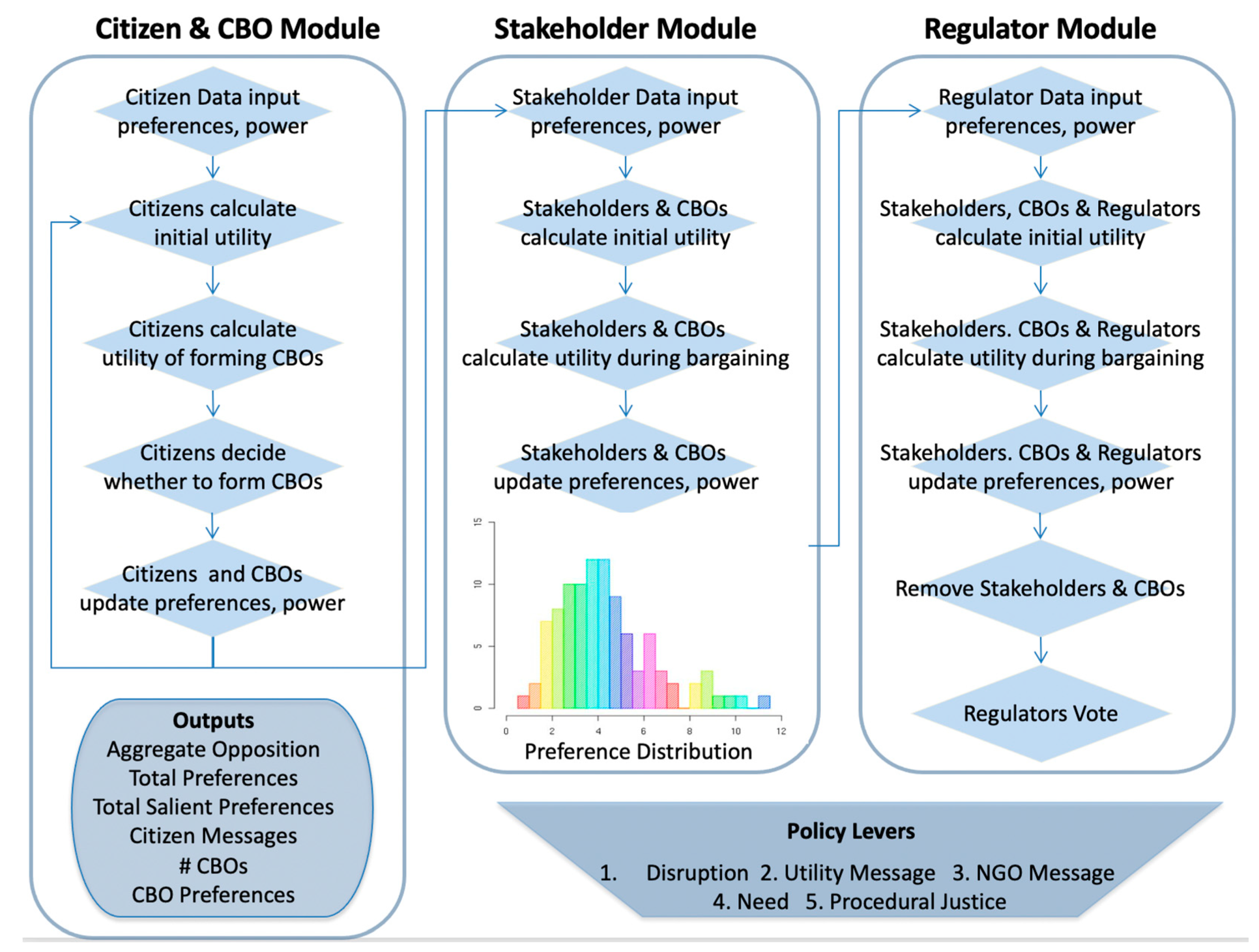
RBEP and SEMPro utilize the ABM-GIS approach to generate evolving, macro-scale system phenomena from the micro-motivations and interactions of computational agents. The pseudo-code and model diagram for SEMPro are detailed in Abdollahian et al. [3]. Nelson et al. document the benefits of integrating GIS with ABMs and evaluate another application of SEMPro [23]. SEMPro is composed of three related modules as detailed in Figure 1.
In the citizen module, each citizen agent is autonomous, with bounded rationality, and maximizes their utility subject to the geophysical, engineering, and social constraints of its system [24]. Agents react to infrastructure siting projects by forming preferences and attempting to influence the preferences of others. Citizen agents send out messages supporting or opposing the project based on their own attributes and proximity to planned infrastructure siting. These citizen interactions can result in the formation of community based organizations (CBOs) that either support or oppose such projects.
To simulate this process, the user loads GIS data and initializes the model. US Census block-group population density data is used to locate citizen agents in the ABM. Citizen agents are instantiated in the model space at a sampled rate consistent with their Census population (i.e., 1 agent per 1000 Census population). US Census data on median educational attainment and income are instantiated as attributes of the agents in the model and provide initial heterogeneity for simulated citizen behavior. Higher education and income affect project outcomes and are described as citizen “power” due to greater perceptions of self-efficacy and resources available for advocacy.
RBEP simulates the technical aspects of the decision process using project engineering and line or polygon GIS data. These represent the proposed the power lines or power plants. The inclusion of GIS project data with the Census data is critical as the project is placed into the “real-world” political and social community attributes. This is critical as infrastructure projects are often sited in an existing right-of-way. The right-of-way represents the setback between the project and the built environment such as residential housing. This drives citizen and subsequent model behavior as the closeness of the citizen agents to the project is the driving parameter in the model [25]. The importance or salience that each citizen attaches to the project is the inverse of their distance to the unwanted land-use. On average, citizens who live further away do not engage in the siting process because it is important. This can be measured as the “half-length” for citizen participation defined as the median distance away from the LULU for citizens’ residences [26].
3.1. Study Area
Redondo Beach is the southernmost of Los Angeles County’s three beach cities, the other two Beach Cities being Hermosa Beach and Manhattan Beach. The Redondo Beach power plant is located in the middle of the City of Redondo Beach. The Redondo Beach power plant has existed in some form or other since around 1897. In 1998, SCE sold the power plant to the AES Corporation who signed a deal with the City of Redondo Beach to downsize the power plant. Within the next couple of years, three of the eight smokestacks had been torn down. The plant was used as a “peaking plant,” i.e., it was only run at times of peak demand for electricity, meaning that the plant had a downtime of over 95 percent.
In 2011, AES filed plans to tear down the entire power plant and build “a brand new power plant that would be cleaner, more efficient, and one-third the size of the current facility” [27]. In proposing this smaller plant, part of the original power plant lot would be unused, and AES proposed rezoning some of the unused land for “community purposes” [28]. Despite being an apparent improvement on existing conditions (a cleaner and more efficient plant and the opening up of land for the community), the plans generated a high degree of opposition from the community, especially from a CBO called Building a Better Redondo. This CBO was started in 2006 to oppose changes to zoning laws in the city and had engaged an extensive network of activists and citizens [29]. Its opposition activities generated many public comments through the environmental impact report process for the project which are used to validate the RBEP model.
3.2. Model Verification
In order for RBEP to provide decision support, users need to be confident in the model’s predictions. For ABMs, as with other non-linear systems, it is crucial to verify the model’s code as even minor mistakes can propagate through the simulation and create major differences in output. In this case, the base SEMPro model has been verified on several previous occasions (in more than 6000 runs) [3,6,23]. Furthermore, as part of the Sustainable Energy Infrastructure project (National Science Foundation award #1737191), SEMPro had two dedicated coders that examined the model and documented problems. This led to several bug fixes, including to the expected utility calculation and the linkages created between citizen agents.
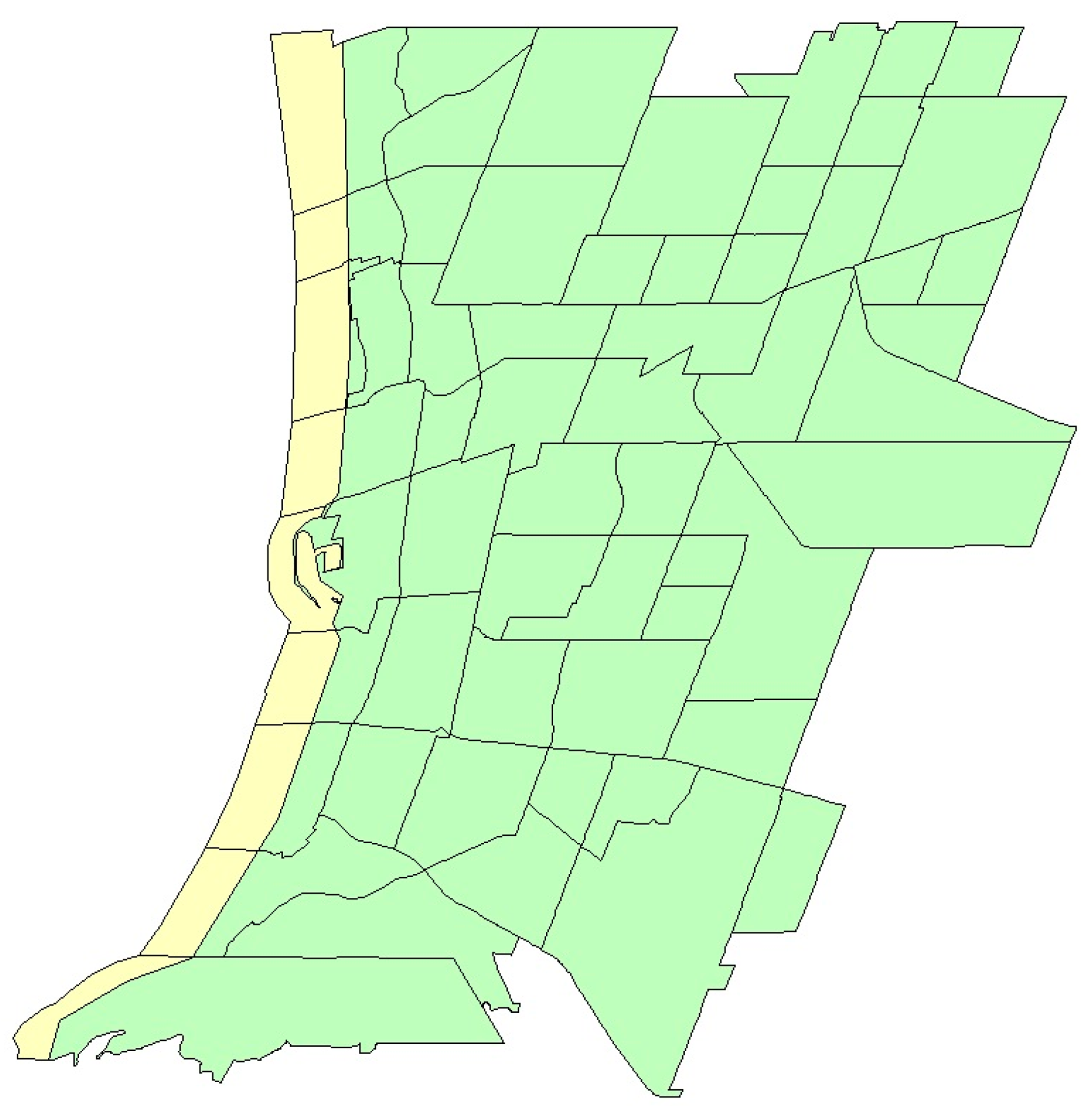
ABMs also need to also be verified against the inclusion of poor-quality data. The verification of the GIS-module for RBEP showed that the US Census data shapefiles did not possess very accurate coastlines. Coastlines were smoothed out to straight lines and often extended into the water. The error can be seen in Figure 2, with the yellow parts on the left side of the map representing the marine areas added to the map. Since part of the agent instantiation process includes calculating the population density of the different Census block groups, the area of the tracts needed to be updated.
To ameliorate this problem, the world water bodies dataset from the ESRI database was used to clip out these extraneous areas [30]. This required some polygons to be split into several pieces and reassembled again. The shapefiles were ultimately revised with accurate areas to use in the calculation of population density and the spatial instantiation of citizen agents in the model.
3.3. Data
Using the pattern-oriented-modeling approach to validation, the model settings were calibrated to fit the RBEP study area. This included using the Census data and calculating the geographic areas and distances. Since the power plant in Redondo Beach has existed in some form for more than 100 years, the disruption variable was kept in the lower range. This is also confirmed by the case study, which showed a long drawn out process consistent with low settings of disruption and no significant change to the land-use of the land (a high setting for the model’s disruption parameter is the equivalent of a dramatic change of land use).
The public Environmental Impact Report (EIR) yielded data on citizen and stakeholder preferences. The comment data stretched from 20 November 2012 up to 28 June 2016. However, the actual EIR timeframe when the comments were taken into active consideration for the project was 20 months and contained 231 citizen comments [31].
The comments from the EIR procedure allowed us to quantify citizen and CBO preferences, as well as to geocode citizen locations. Validation includes a direct comparison of modeled outputs with the results of the actual project. This increases the confidence in the validation procedures.
The model was run with two different settings for the connectedness of citizen agents. Talk-span represents the importance of in-person communication as identified in the literature [32,33]. Average talk-span values reflect a mix of face-to-face communication as well as more modern communication methods like email and social media. Given the activities of the Building a Better Redondo CBO, actual citizen connectedness was likely to be best represented by the average values of the talk-span parameter. The low talk-span dataset was also used for further validation of the model predictions against the historical dataset.
4. Results
The validation outputs for real citizens comments as well as low and average talk-span parameter settings are divided into three categories: pattern-oriented maps, global spatial statistics, and local spatial statistics.
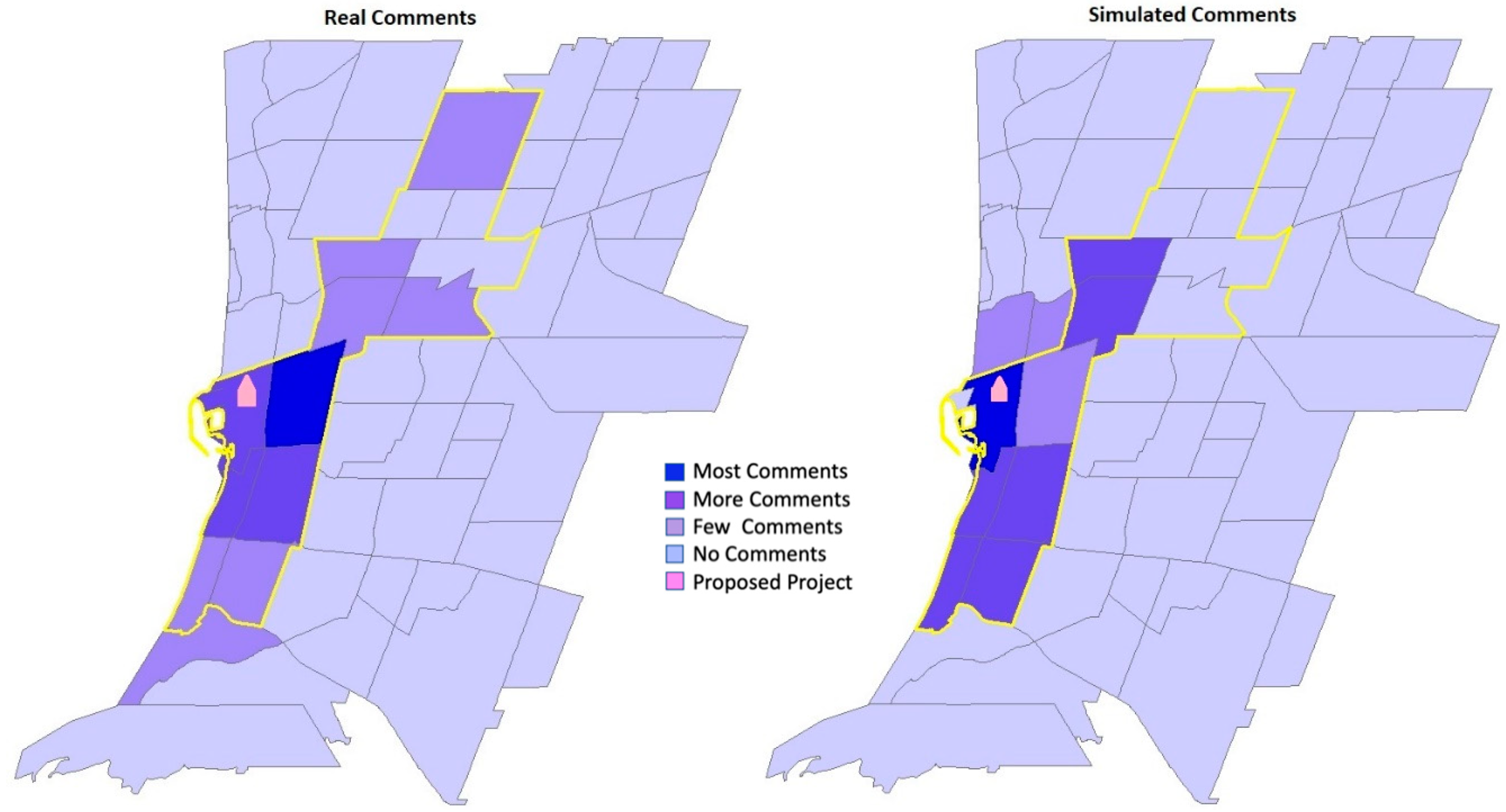
Figure 3 displays the pattern-oriented results of the low talk-span settings, with the real comments on the left map and the simulated comments on the right map. The low talk-span setting in the RBEP simulations underpredicted citizen comments in Census tracts to the far north and south of the real comments. The simulations also overpredicted citizen comments in the Census tracts adjacent to and just north of the proposed project (dark purple).
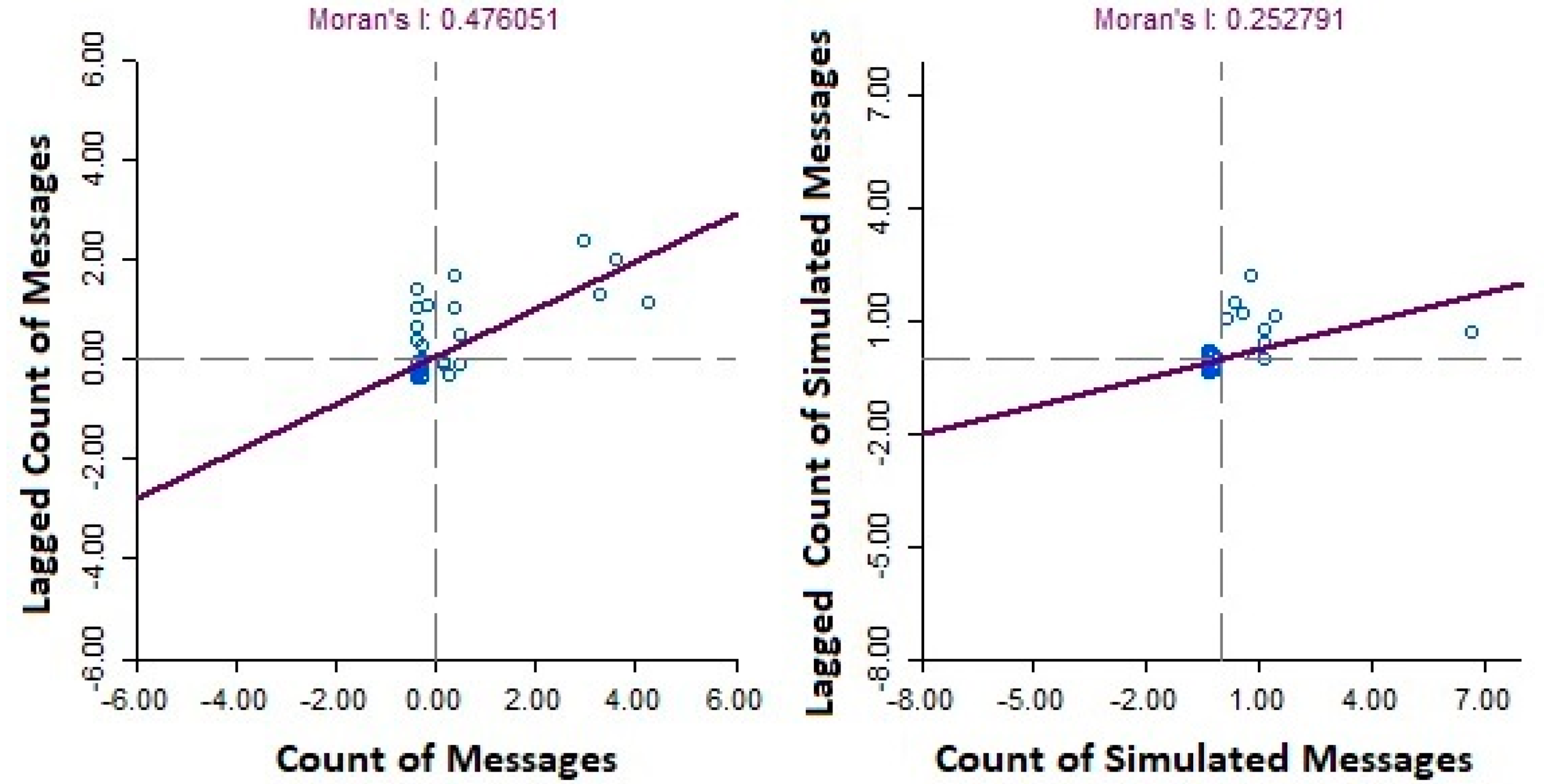
Overall, the model’s simulated comments display a high level of similarity with the real comments. Figure 4 shows that the global Moran’s I for the real comments was 0.48 and for the simulated comments it was 0.25. While the two Moran’s I coefficients display some variation, it is evident that the bulk of observations is clustered around the origin of the X-axis in both graphs.
The second parameter setting for citizen connectedness was with talk-span levels averaged over a range of talk-span settings (i.e., the model was run at several different talk-span settings and then consolidated into one dataset). The results of this can be seen in Figure 5.
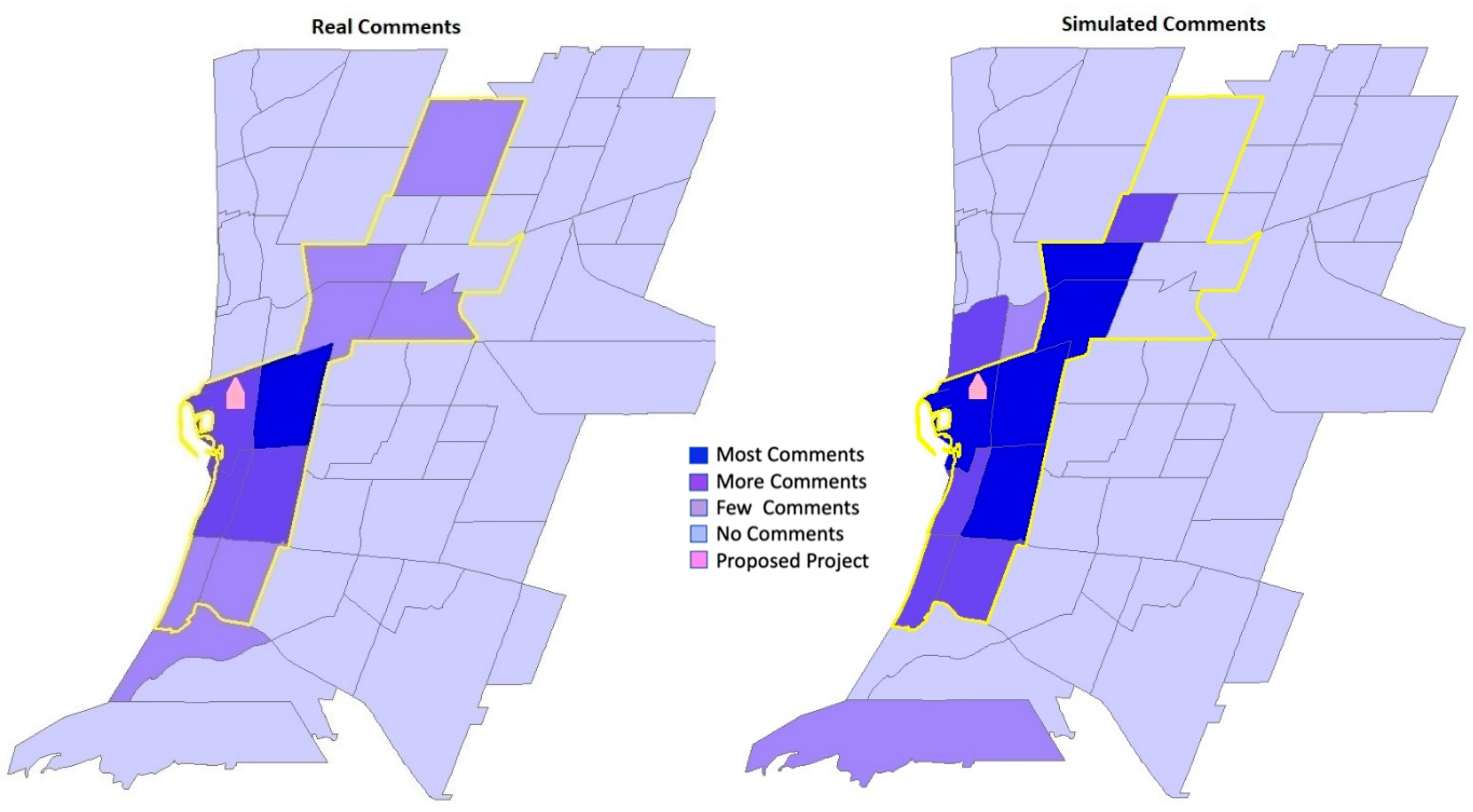
Figure 5 presents a slight bias for overpredictions in the average talk-span setting. The pattern of the simulated comments looks quite similar to the real comments pattern, but there is a higher concentration of messages in the areas immediately to the east, northeast, and southeast.
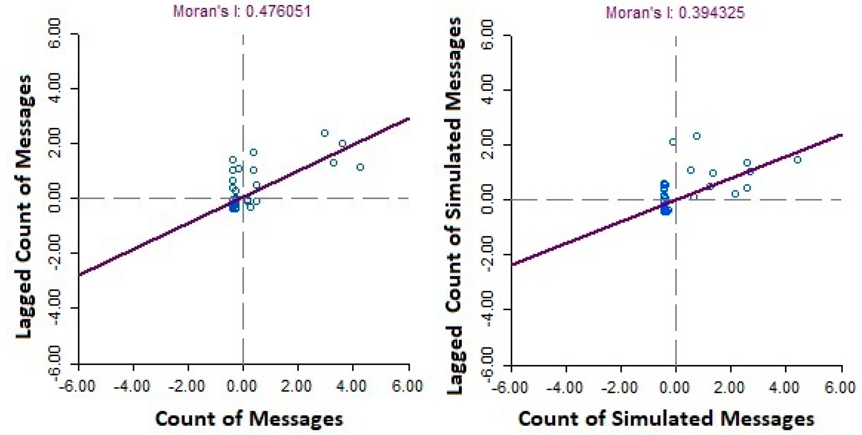
Furthermore, the Moran’s I comparison, shown in Figure 6, shows a higher level of spatial auto-correlation, with scores of 0.48 for the real comments (L) and 0.39 for the simulated comments (R). The Moran’s I was higher for the average talk-span data than for the low talk-span (Figure 4), indicating the setting is more reflective of the real-world data generating process. The average talk span setting results in citizen comments that extend spatially out from the origin and to the right as can be seen in the comparison of the right panels in Figure 4 and Figure 6.
In order to extend the spatial validation analyses, bivariate correlations were performed. These test the correlations between the real comments and the predicted comments by summing up all the comments in each Census block group (N = 58) for each of the three datasets: the two talk-span outputs and the real comments. The results of this pairwise test can be seen in Table 1.
The results of the bivariate correlation show that the model performs best with the average talk-span setting. Under these settings, the model explains about 65% of the variation in the historical citizen comments.
4.1. Local Indicators of Spatial Association Results
A comparison of the choropleth maps in Figure 3 and Figure 5 with Moran’s I plots in Figure 4 and Figure 6 illuminates Costanza’s [34] claim that statistics alone are not enough. In this case, the Moran’s I results do not paint a clear enough picture by themselves. For instance, while the statistics suggest a level of global spatial autocorrelation, and whether it is positive or negative, they do not tell us about where the messages are located in space. Are the messages close to the plant or somewhere else? Are there distinct patterns, and do certain local geographies over or under perform?
The final validation test used the GeoDa software to create cluster and significance maps for the different datasets. The local Moran’s I or the local indicators of spatial association (LISA) statistic was used to test for clustering in the spatial arrangements of the real and simulated phenomena. In this case, the LISA statistic measures spatial autocorrelation at the Census tract level. This provides higher resolution than the Moran’s I clustering statistic for the entire area. Like other statistical measures, LISA consists of two results: (1) a test statistic as well as (2) its statistical significance which identifies the probability of the result happening as a result of chance.
First, the LISA statistics allow the identification of areas with high or low values of messages, as well as if they had neighbors with high or low values. If a Census tract has a high number of citizens that sent messages, it will be classified as “High” and be colored in vibrant red. If a “High” area also has neighbors that are “High”, it will be classified as a “High-High” area. For areas with low values of messages, it works the same, except the color is solid blue and the areas are called “Low-Low”. The other 3 categories are mixes, i.e., “High-Low” and “Low-High”, as well as an area of no significance. The LISA indicator thus gives us a measure of the clustering of messages, as well as information on neighboring tracts’ similarities.
Second, LISA tests the statistical significance of the tracts’ clustering compared to random distributions. Lighter colors denote a statistically significant contribution towards negative spatial autocorrelation, whereas the solid colors denote a statistically significant contribution towards positive spatial autocorrelation. The statistical level of these contributions can be seen in the significance maps below.
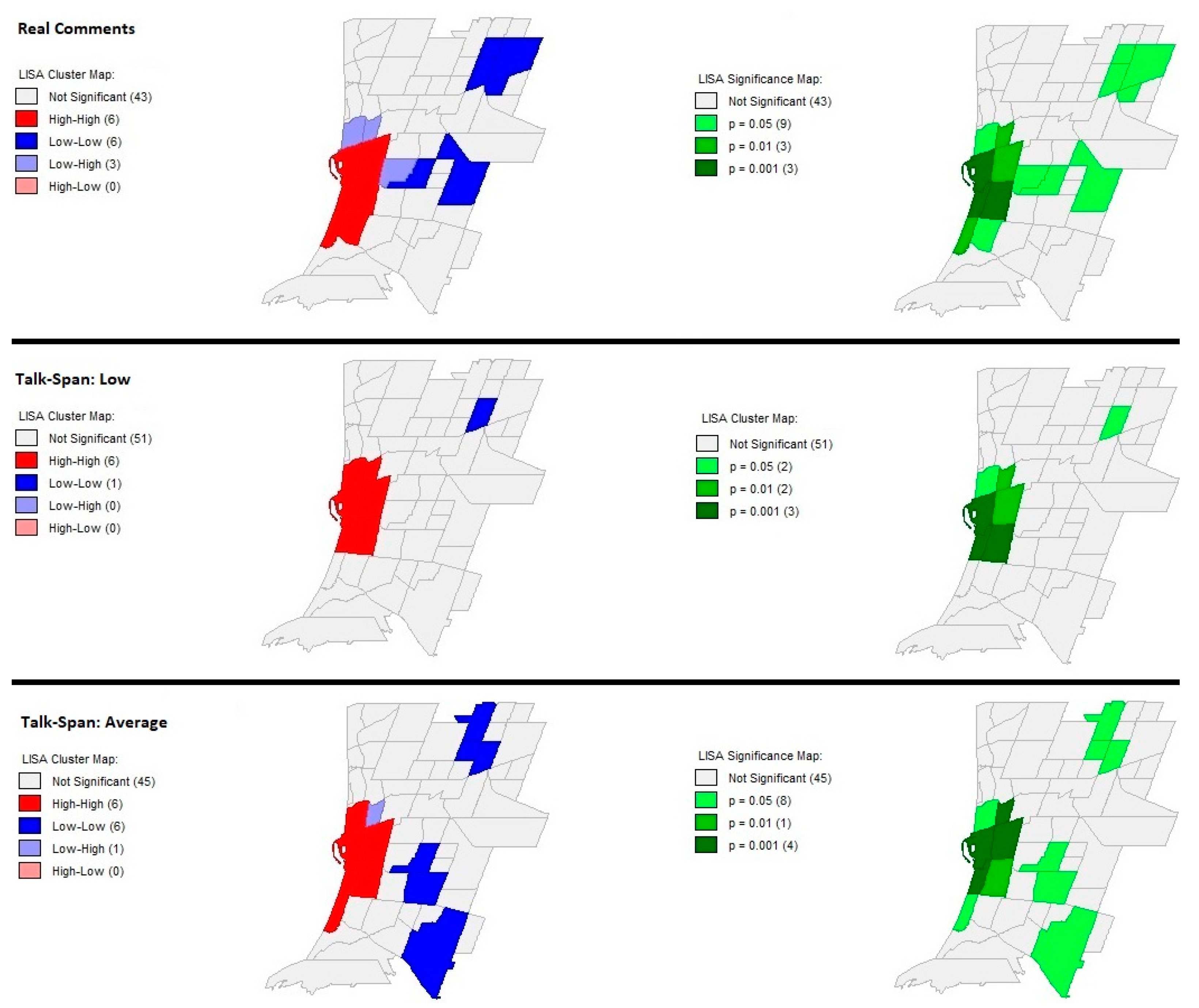
The cluster maps in Figure 7 show that the use of the low talk-span parameter value does not allow citizen agents to communicate across Census tracts as was done historically with help from the local opposition CBO. Most of the non-proximate historical comments are in the portion of Redondo Beach that was perceived to be in the neighborhoods that are “downwind” and to the east of the natural gas plant’s projected air pollution emissions.
Using average values for the talk-span parameter, the RBEP model correctly identifies five out of the top six areas of opposition. This setting predicts comments downwind of the LULU and are further away from the proposed power plant. The predictions also reflected a similarity with real comments in the Low-Low areas, correctly predicting about 50% of these areas. Overall, the model’s predictive accuracy is better using this parameter value than the low talk-span value.
4.2. Discussion
The pattern-oriented modeling techniques developed for this paper offer several insights for the field of the validation of ABM-GIS models. First, integrated ABM-GIS models that offer decision support often include representation of social, institutional, and geophysical factors in the model. For these complex models, validation against historical data is almost certainly required to generate user buy-in on the model’s efficacy. In other worlds, the stronger the theoretical linkages between the real and simulated worlds, the greater the need for robust tests of those same empirical linkages. The mapping tools developed for the pattern-oriented modeling approach help identify the real-world data generating process and are intuitive for stakeholders to utilize [13,14].
Second, the selection of spatial statistics with which to test linkages between real and predicted outcomes is dependent on the real-world data generating process [7]. For real-world processes that generate a uniform distribution of phenomena, a global test like Moran’s I is probably adequate. Processes that generate outliers and clusters require a local test. Fortunately, the time to generate an additional test in most GIS software is minimal for most advanced users.
Third, the two spatial statistics offer different insights into the model’s predictions. The higher values of the global Moran’s I for the higher talk-span setting (0.39) showed that it better represented real-world global citizen connectedness (0.48) than the lower talk-span setting (0.25). Sensitivity runs for other key parameters in the model can similarly help to calibrate parameter settings. This calibration is important to improve the realism of the ABM-GIS models [18]. Calibration efforts can include the use of bivariate correlations to estimate goodness of fit statistics like percentage of variance explained (R2) as demonstrated in Table 1.
The LISA statistic offered theoretical insights into the model’s specification [20]. LISA identified areas of both positive and negative local clustering in both the real and simulated results. The positive clustering areas represented the High-High hot spots near the proposed power plant. The negative areas represented the Low-Low or cold spots distant from the proposed source of unwanted air pollution. These areas likely have attributes that are not captured in the existing model. For instance, the RBEP does not explicitly include city boundaries. However, the city was a vocal opponent of the power plant and communicated this to its residents. The citizens in Census tracts adjacent to the north of the plant and outside of the city did not comment on the EIR (Figure 5), while the RBEP model predicted substantial comments. Similarly, LISA identified cold spots east and downwind of the plant. The LISA results indicate that these biases in the results are probably due to the fact that these tracts are outside of the City of Redondo Beach and not a part of the city’s communication, electoral, and advocacy networks. Future improvements to the model should likely include a parameter for citizen location inside/outside of the city boundaries in its communication network representation.
5. Conclusions
One of the most distinctive takeaways from the literature review is the need for a comprehensive validation process. The results presented above agree that in the majority of spatial validation cases there will not be one “silver-bullet” statistic that will crown a spatially explicit ABM as properly validated. Instead, researchers have to utilize different tools and techniques to establish an acceptable degree of validity based on the structure and the purpose of the model. Validating ABM models in general, and especially with integrated ABM-GIS models, is an exercise in epistemological reasoning as these models explicitly link the simulated world with the real world [35]. This research started with pattern-oriented modeling, and then used spatial autocorrelation statistics to operationalize and test global as well as local clustering of citizen comments.
Furthermore, a model may have key parameters that need to be calibrated in order to maximize the similarity of predictions to the real-world data generating process. This research found that model calibration can be informed through the global spatial autocorrelation test and bivariate correlation tests. These were applied to the different outputs of the talk-span parameter, a global parameter in the RBEP model. The LISA tests identified hot spots where citizens who lived close to the proposed LULU were more likely to submit written comments as well as cold spots outside the City of Redondo Beach that did not generate anticipated citizen activity. The multi-stage validation thus provided important insights into the real-world complex adaptive systems that the spatially-explicit ABM is intended to parsimoniously depict. Considering the increasing trend towards a higher “level of realism in representing space” [18] (p. 253), the results also emphasize the importance of spatial validation. The use of realistic representations of space without validation can lead to seriously misleading results and policy recommendations. Conversely, correct spatial validation can lead to increased confidence in the model, as well as increased utility of the results by decisionmakers.
Author Contributions
K.W.: Conceptualization, Formal analysis, Funding acquisition, Investigation, Methodology, Project administration, Visualization, Resources, Supervision, Validation, Visualization, Writing—original draft, Writing—review & editing. Formal analysis. H.T.N.: Formal analysis, Investigation, Methodology, Visualization, Supervision, Project administration, Writing—review & editing. All authors have read and agreed to the published version of the manuscript.
Funding
This research was supported by the Haynes Foundation under the Power Struggles grant and via a dissertation fellowship, as well as the National Science Foundation grant #1737191. The funders had no influence on the content of this article or on the selection of the journal for publication.
Institutional Review Board Statement
No institutional approvals were required as a part of this research.
Informed Consent Statement
Informed consent was required as a part of this research.
Data Availability Statement
Data for this research is not available.
Conflicts of Interest
Nelson is a principal in the firm that developed the SEMPro software.
References
- Axelrod, R. Advancing the Art of Simulation in the Social Sciences. In Simulating Social Phenomena; Conte, R., Hegselmann, R., Terna, P., Eds.; Springer: Berlin, Germany, 1997; pp. 21–40. [Google Scholar]
- Regan, H.M.; Colyvan, M.; Burgman, M.A. A taxonomy and treatment of uncertainty for ecology and conservation biology. Ecol. Appl. 2002, 12, 618–628. [Google Scholar] [CrossRef]
- Abdollahian, M.; Yang, Z.; Nelson, H. Sustainable Energy Modeling Programming (SEMPro). J. Artif. Soc. Soc. Simul. 2013, 16, 6. Available online: http://jasss.soc.surrey.ac.uk/16/3/6.html (accessed on 14 June 2014). [CrossRef]
- Vespignani, A. Predicting the behavior of techno-social systems. Science 2009, 325, 425–428. [Google Scholar] [CrossRef] [PubMed]
- Quek, H.Y.; Tan, K.C.; Abbass, H.A. Evolutionary game theoretic approach for modeling civil violence. IEEE Comput. 2009, 13, 780–800. [Google Scholar]
- Yang, Z.; Nelson, H.T.; Abdollahian, M. Sustainable Energy Infrastructure Siting: An Agent Based Approach. J. Energy Chall. Mech. 2015, 75–84. Available online: https://www.researchgate.net/publication/301493902_Sustainable_Energy_Infrastructure_Siting_An_Agent_Based_Approach (accessed on 19 October 2022).
- Fagiolo, G.; Moneta, A.; Windrum, P. A Critical Guide to Empirical Validation of Agent-Based Models in Economics: Methodologies, Procedures, and Open Problems. Comput. Econ. 2007, 30, 195–226. [Google Scholar] [CrossRef]
- Levy, S.; Martens, K.; Van Der Heijden, R. Agent-based models and self-organisation: Addressing common criticisms and the role of agent-based modelling in urban planning. Town Plan. Rev. 2016, 87, 321–338. [Google Scholar] [CrossRef]
- Heppenstall, A.; Malleson, N.; Crooks, A. “Space, the Final Frontier”: How Good are Agent-Based Models at Simulating Individuals and Space in Cities? Systems 2016, 4, 9. [Google Scholar] [CrossRef] [Green Version]
- Sun, Z.; Müller, D. A framework for modeling payments for ecosystem services with agent-based models, Bayesian belief networks and opinion dynamics models. Environ. Model. Softw. 2013, 45, 15–28. [Google Scholar] [CrossRef]
- Schulze, J.; Müller, B.; Groeneveld, J.; Grimm, V. Agent-Based Modelling of Social-Ecological Systems: Achievements, Challenges, and a Way Forward. J. Artif. Soc. Soc. Simul. 2017, 20, 8. [Google Scholar] [CrossRef] [Green Version]
- Chattoe-Brown, E. A Bibliography of ABM Research Explicitly Comparing Real and Simulated Data for Validation. Review of Artificial Societies and Social Simulation. 12 June 2020. Available online: http://cfpm.org/discussionpapers/256 (accessed on 2 November 2022).
- Sargent, R.G. Validation and verification of simulation models. In Proceedings of the 36th Conference on Winter Simulation, Washington, DC, USA, 5–8 December 2004; pp. 17–28. [Google Scholar]
- Duong, D. Verification, Validation, and Accreditation (VV&A) of Social Simulations. In Spring Simulation Interoperability Workshop, Orlando; 2010; Available online: https://core.ac.uk/download/pdf/36723553.pdf (accessed on 19 October 2022).
- Kang, J.-Y.; Aldstadt, J. Using multiple scale spatio-temporal patterns for validating spatially explicit agent-based models. Int. J. Geogr. Inf. Sci. 2019, 33, 193–213. [Google Scholar] [CrossRef]
- Grimm, V.; Revilla, E.; Berger, U.; Jeltsch, F.; Mooij, W.M.; Railsback, S.F.; Thulke, H.H.; Weiner, J.; Wiegand, T.; DeAngelis, D.L. Pattern-Oriented Modeling of Agent-Based Complex Systems: Lessons from Ecology. Science 2005, 310, 987–991. [Google Scholar] [CrossRef]
- Grimm, V.; Railsback, S.F. Pattern-oriented modelling: A ‘multi-scope’ for predictive systems ecology. Philos. Trans. R. Soc. B Biol. Sci. 2012, 367, 298–310. [Google Scholar] [CrossRef] [Green Version]
- Stanilov, K. Space in agent-based models. In Agent-Based Models of Geographical Systems; Springer: Dordrecht, The Netherlands, 2012; pp. 253–269. [Google Scholar]
- Pontius, R.G. Quantification error versus location error in comparison of categorical maps. Photogramm. Eng. Remote Sens. 2000, 66, 1011–1016. [Google Scholar]
- Brown, D.G.; Page, S.; Riolo, R.; Zellner, M.; Rand, W. Path dependence and the validation of agent-based spatial models of land use. Int. J. Geogr. Inf. Sci. 2005, 19, 153–174. [Google Scholar] [CrossRef] [Green Version]
- Crooks, A.T.; Heppenstall, A.J. Introduction to agent-based modelling. In Agent-Based Models of Geographical Systems; Springer: Dordrecht, The Netherlands, 2012. [Google Scholar]
- Law, A.; Kelton, D.W. Simulation Modeling and Analysis (Industrial Engineering and Management Science Series); McGraw-Hill Higher Education: New York, NY, USA, 1999. [Google Scholar]
- Nelson, H.; Cain, N.L.; Yang, Z. All politics is spatial: Integrating an agent-based model with spatially explicit landscape data. In Rethinking Environmental Justice in Sustainable Cities; Routledge: London, UK, 2015; pp. 190–211. [Google Scholar]
- Yeung, C.; Poon, A.; Wu, F. Game theoretical multi-agent modelling of coalition formation for multilateral trades. IEEE Trans. Power Syst. 1999, 14, 929–934. [Google Scholar] [CrossRef] [Green Version]
- Nelson, H.T.; Swanson, B.; Cain, N.L. Close and Connected: The Effects of Proximity and Social Ties on Citizen Opposition to Electricity Transmission Lines. Environ. Behav. 2018, 50, 567–596. [Google Scholar] [CrossRef]
- Nelson, H.T.; Wikstrom, K.; Hass, S.; Sarle, K. Half-length and the FACT framework: Distance-decay and citizen opposition to energy facilities. Land Use Policy 2021, 101, 105101. [Google Scholar] [CrossRef]
- Gnerre, S. Redondo Beach’s Power Plants. 5 October 2011. Available online: http://blogs.dailybreeze.com/history/2011/10/05/redondo-beachs-power-plant/ (accessed on 23 June 2020).
- AES California. (ND) Frequently Asked Questions. Available online: http://aescalifornia.com/files/pdf/top-rb-faqs-final.pdf (accessed on 24 June 2020).
- Building a Better Redondo. About Us. 2022. Available online: https://buildingabetterredondo.org/bbr_about.html (accessed on 2 November 2022).
- ArcGIS Hub. World Water Bodies. 2022. Available online: https://hub.arcgis.com/content/esri::world-water-bodies/about (accessed on 26 June 2018).
- California Energy Commission. Docket Log 12-AFC-03. Available online: https://efiling.energy.ca.gov/Lists/DocketLog.aspx?docketnumber=12-AFC-03 (accessed on 18 September 2018).
- Kasperson, R.E.; Renn, O.; Slovic, P.; Brown, H.S.; Emel, J.; Goble, R.; Kasperson, J.X.; Ratick, S. The Social Amplification of Risk: A Conceptual Framework. Risk Anal. 1988, 8, 177–187. [Google Scholar] [CrossRef] [Green Version]
- Trumbo, C.W. Examining psychometrics and polarization in a single-risk case study. Risk Anal. 1996, 16, 429–438. [Google Scholar] [CrossRef]
- Costanza, R. Model goodness of fit: A multiple resolution procedure. Ecol. Model. 1989, 47, 199–215. [Google Scholar] [CrossRef]
- Graebner, C. How to Relate Models to Reality? An Epistemological Framework for the Validation and Verification of Computational Models. J. Artif. Soc. Soc. Simul. 2018, 21, 8. [Google Scholar] [CrossRef]
Figure 1.
RBEP/SEMPro model diagram.

Figure 2.
Coastal clipping of the US Census shapefiles. The yellow color highlights the marine areas that had to be cut out of the GIS data in order to get an accurate representation of the geographical space.
Figure 2.
Coastal clipping of the US Census shapefiles. The yellow color highlights the marine areas that had to be cut out of the GIS data in order to get an accurate representation of the geographical space.

Figure 3.
Real comments from the RBEP (L) vs. low talk-span simulated comments (R) from the RBEP-model. The yellow lines outline the Redondo Beach city limit. Comments are measured as the total number of comments per Census block group.
Figure 3.
Real comments from the RBEP (L) vs. low talk-span simulated comments (R) from the RBEP-model. The yellow lines outline the Redondo Beach city limit. Comments are measured as the total number of comments per Census block group.

Figure 4.
Moran’s I scores for the real (left) and simulated (right) comments with low talk-span.

Figure 5.
Real (L) vs. average talk-span simulated comments (R). The yellow lines outline the Redondo Beach city limit. Comments are measured as the total number of comments per Census block group.
Figure 5.
Real (L) vs. average talk-span simulated comments (R). The yellow lines outline the Redondo Beach city limit. Comments are measured as the total number of comments per Census block group.

Figure 6.
Moran’s I scores for real (left) vs. simulated (right) comments, at average talk-span.

Figure 7.
LISA comparison of historic (top) and simulated comments.


Table 1.
Correlation coefficients between historical and simulated comments.
| Correlation with Historical Comments | R2 | N | |
|---|---|---|---|
| Low Talk-Span | 0.70 | 0.49 | 58 |
| Average Talk-Span | 0.81 | 0.65 | 58 |
Publisher’s Note: MDPI stays neutral with regard to jurisdictional claims in published maps and institutional affiliations. |
© 2022 by the authors. Licensee MDPI, Basel, Switzerland. This article is an open access article distributed under the terms and conditions of the Creative Commons Attribution (CC BY) license (https://creativecommons.org/licenses/by/4.0/).
Share and Cite
MDPI and ACS Style
Wikstrom, K.; Nelson, H.T. Spatial Validation of Agent-Based Models. Sustainability 2022, 14, 16623. https://doi.org/10.3390/su142416623
AMA Style
Wikstrom K, Nelson HT. Spatial Validation of Agent-Based Models. Sustainability. 2022; 14(24):16623. https://doi.org/10.3390/su142416623
Chicago/Turabian StyleWikstrom, Kristoffer, and Hal T. Nelson. 2022. "Spatial Validation of Agent-Based Models" Sustainability 14, no. 24: 16623. https://doi.org/10.3390/su142416623
Note that from the first issue of 2016, this journal uses article numbers instead of page numbers. See further details here.