


Impact of Landscape Factors on Automobile Road Deformation Patterns—A Case Study of the Almaty Mountain Road

 ,
,
Abstract
:1. Introduction
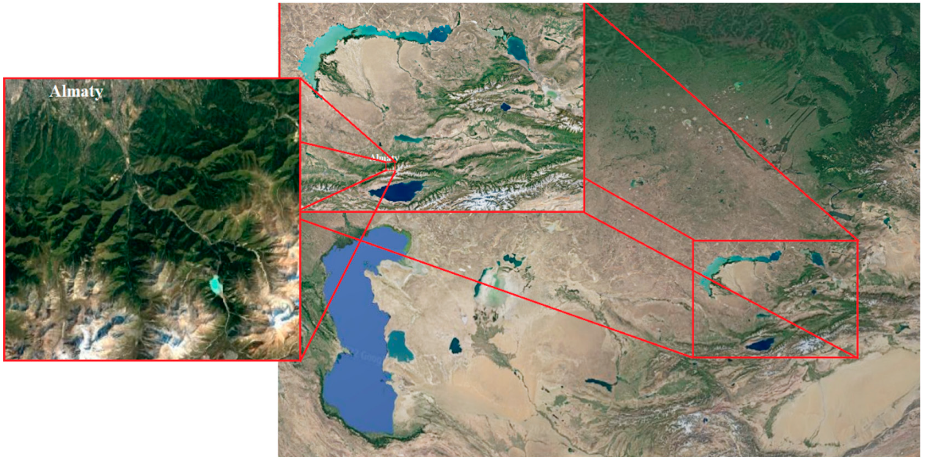
2. Study Area
2.1. General Geographical Charateristics of the Region
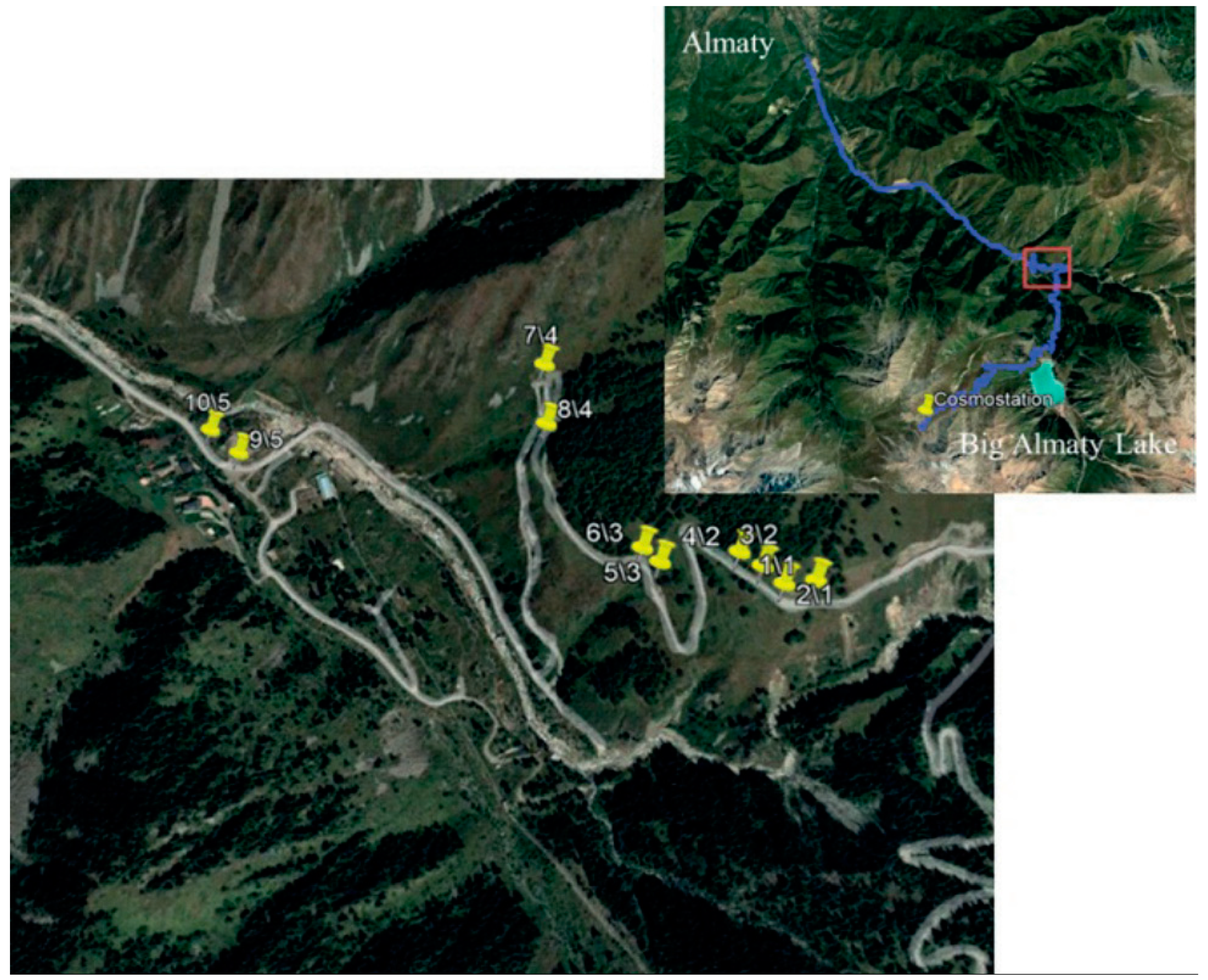
2.2. Characteristics of the Research Area
3. Methodology
3.1. Road Diagnostic Methodology
- The roadbed is solid, the transversal profile is preserved, road cover deformation and defects are absent, and single cracks at intervals of more than 40 m are permissible;
- Between 5% and 30% deformed cover (specified for each cover type) showing inadequate strength of the roadbed, single transversal profile distortion;
- Clear deformations several-fold more severe showing the inadequate strength of the roadbed, unstable holes in crack networks, and occasional ruptures.
- Smooth cover, no deformations;
- Smooth cover with occasional rare deformations not affecting traffic conditions, velocity, or safety;
- The road has small unevenness, widely spaced cracks, and an insignificant number of other deformations;
- The road has significant unevenness, corrugations, raveling, and other deformations affecting traffic conditions and velocity. In addition, edge failures in the road cover are possible [30].
- Visual assessment of the road pavement and road bed;
- Measurement of the road’s transversal and longitudinal unevenness at three points (beginning, middle, and end) using a 3 m-long staff;
- Measurement of the road bed depth;
- Measurement of the pavement’s transversal and longitudinal friction coefficient using a portable IKSp device;
- Measurement of the road pavement’s hardness using a BeldorNII durometer;
- Assessment of the pavement’s width using a sliding caliper;
- Assessment of the transversal, longitudinal, and diagonal crack lengths using a measuring tape and curvimeter.
3.2. Meteorological Impact
- Extremely high temperatures (above 30 °C);
- Extremely low temperatures (less than −15 °C);
- Freezing and thawing cycles;
- Solar radiation;
- Air humidity;
- Highly intensive rainfall (more than 30 mm in 3 h);
- Long but non-intensive rainfall.
3.3. Remotely Sensed Parameter Choice
- Terrain amplitude rise and height decrease at the highest point (i.e., in the source or depletion region);
- Reduction in both amplitude and height at the base of a landslide deposit;
- Growth of amplitude and height in a lower part (i.e., setting zone) [44].
- Vertical displacements with coherent points;
- Slope exposure;
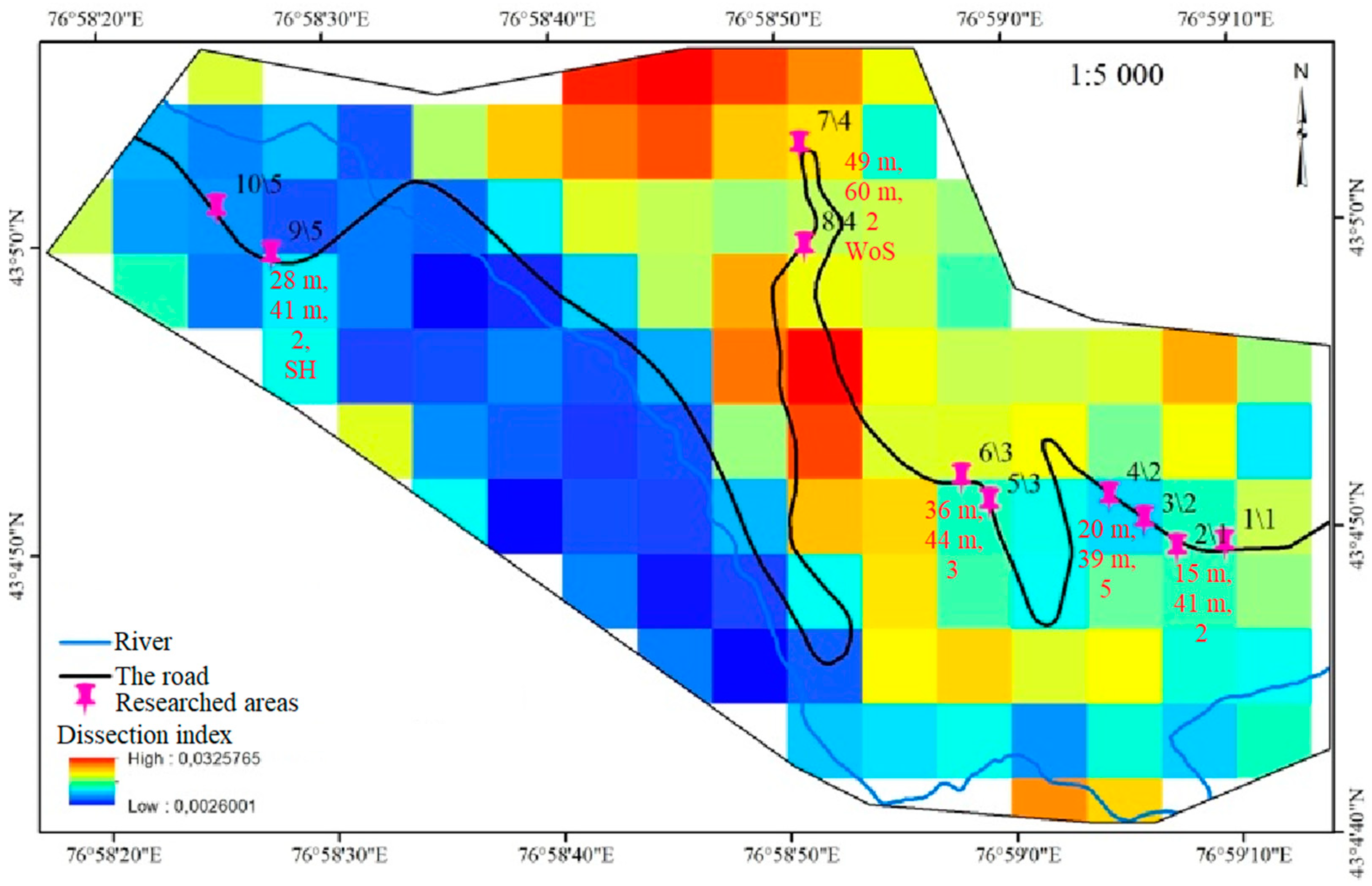
- Dissections;
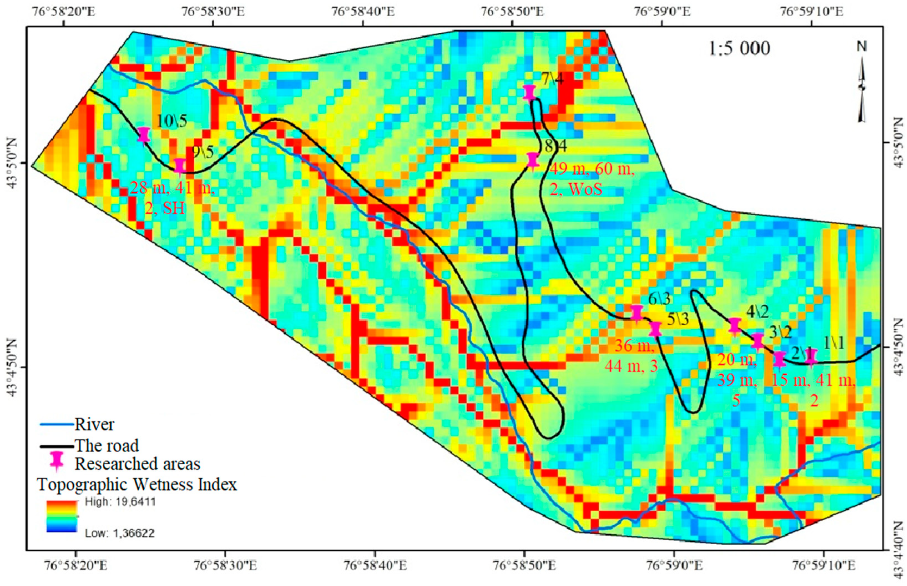
- Topographic wetness index;
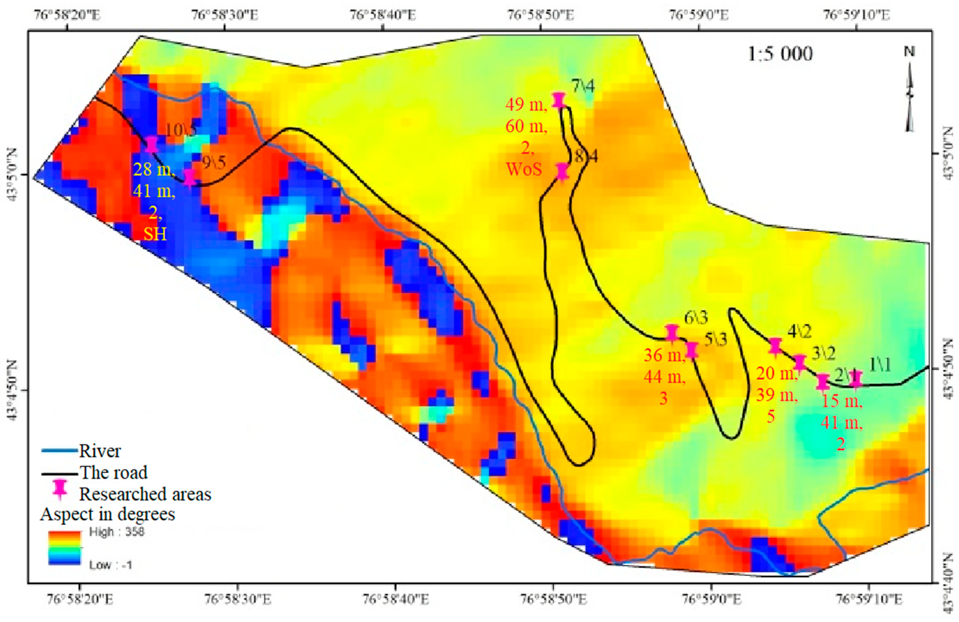
- Aspect;
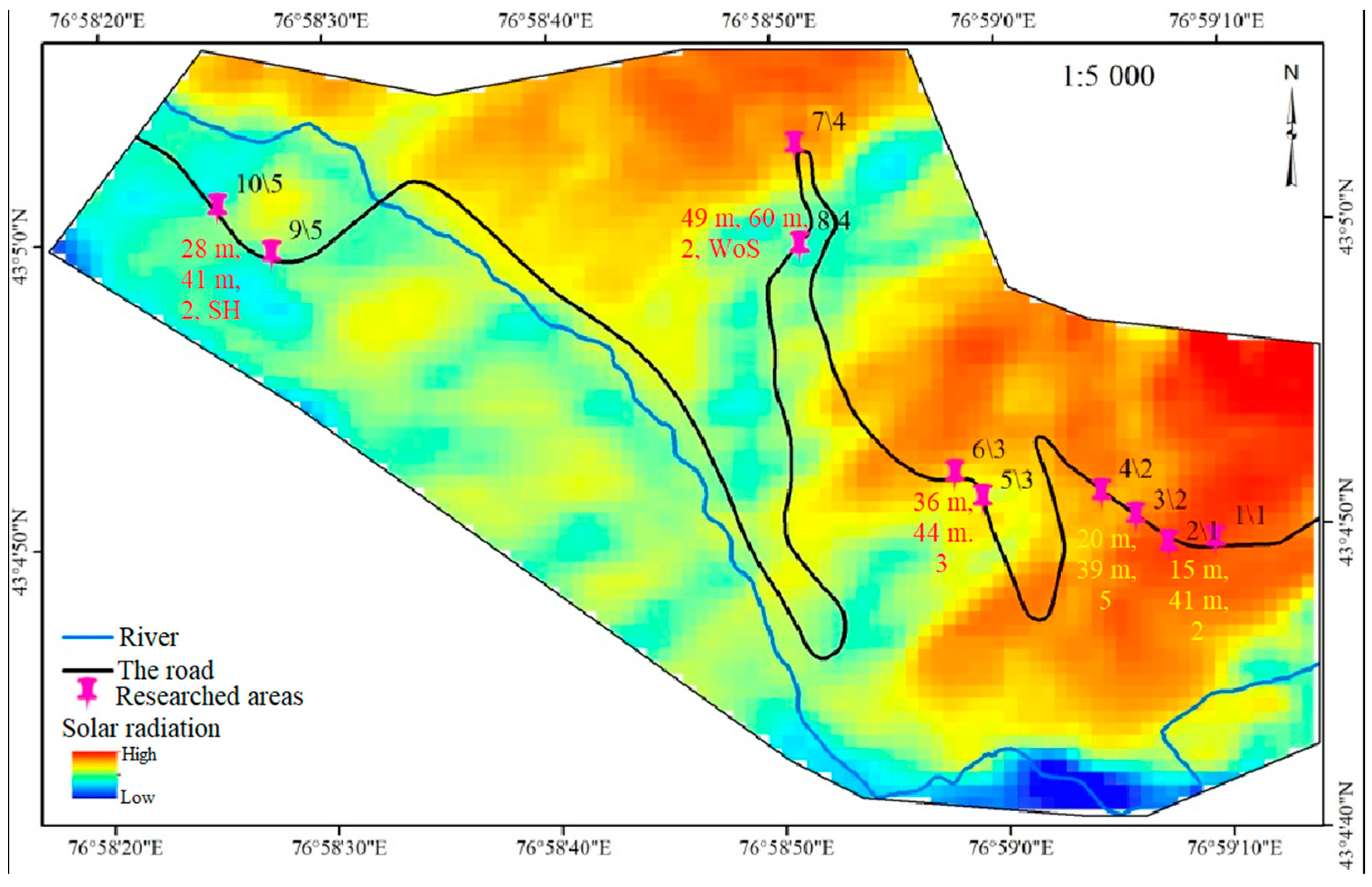
- Solar radiation;
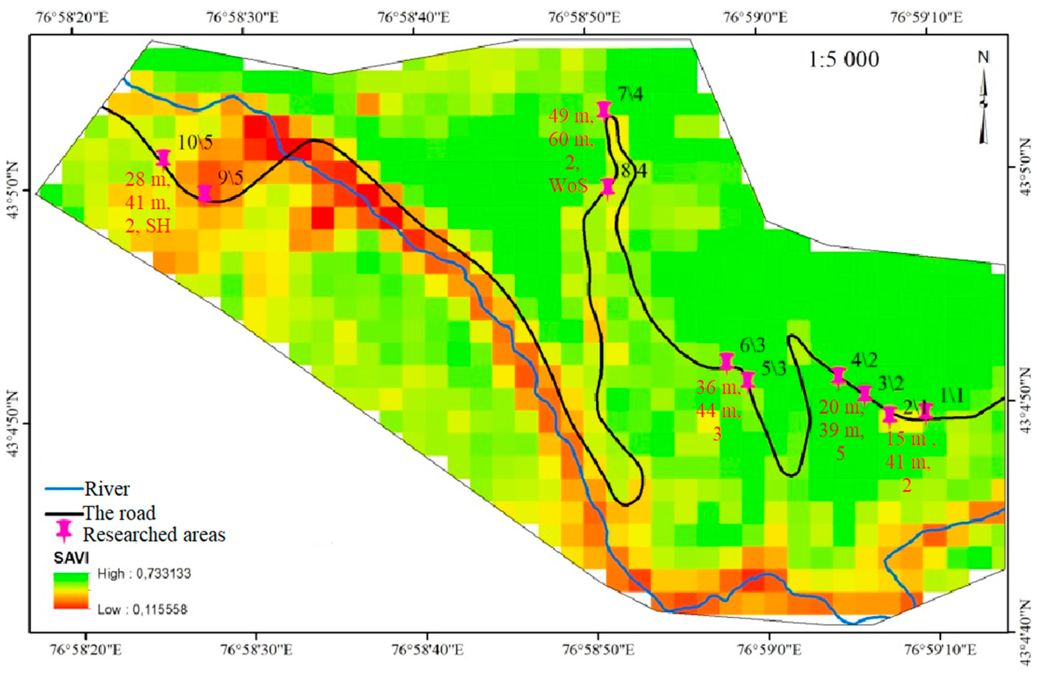
- Vegetation index SAVI;
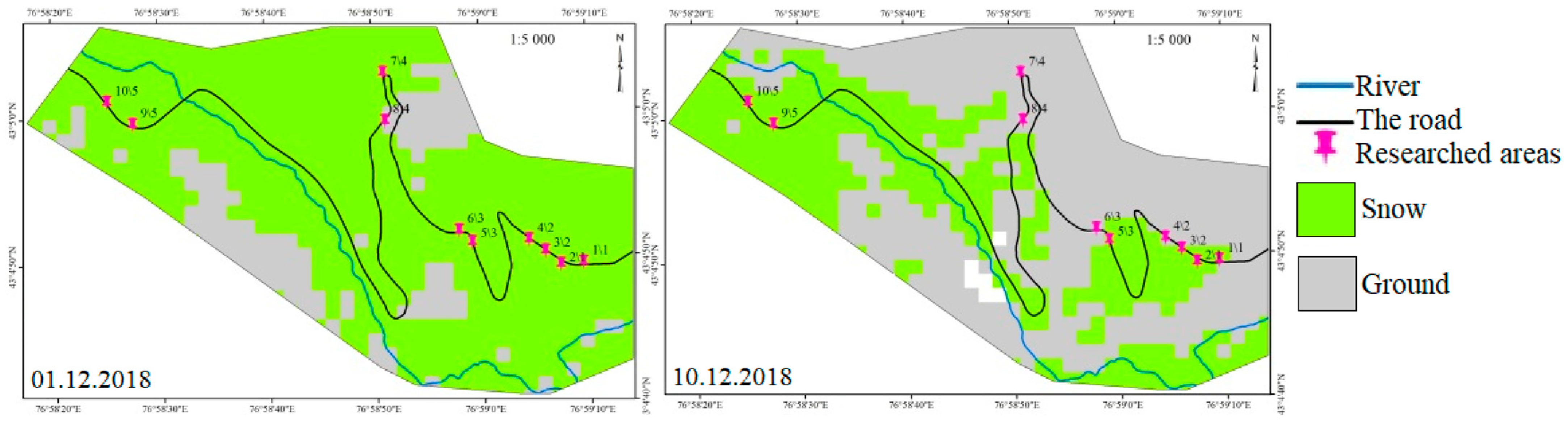
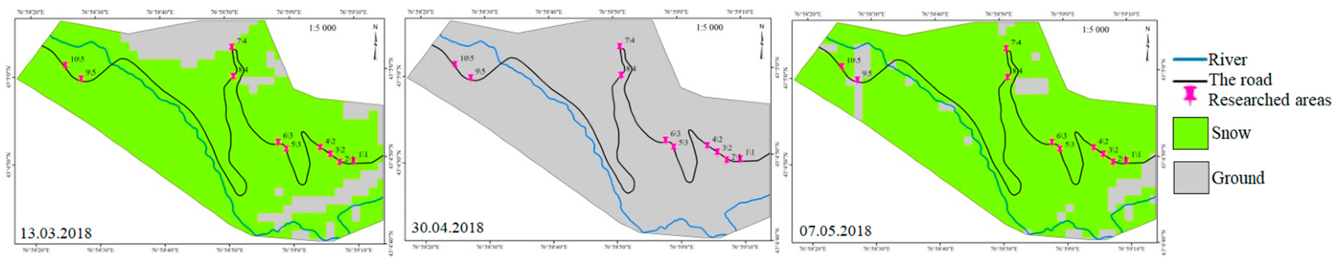
- Snow-covered zones.
4. Results and Discussion
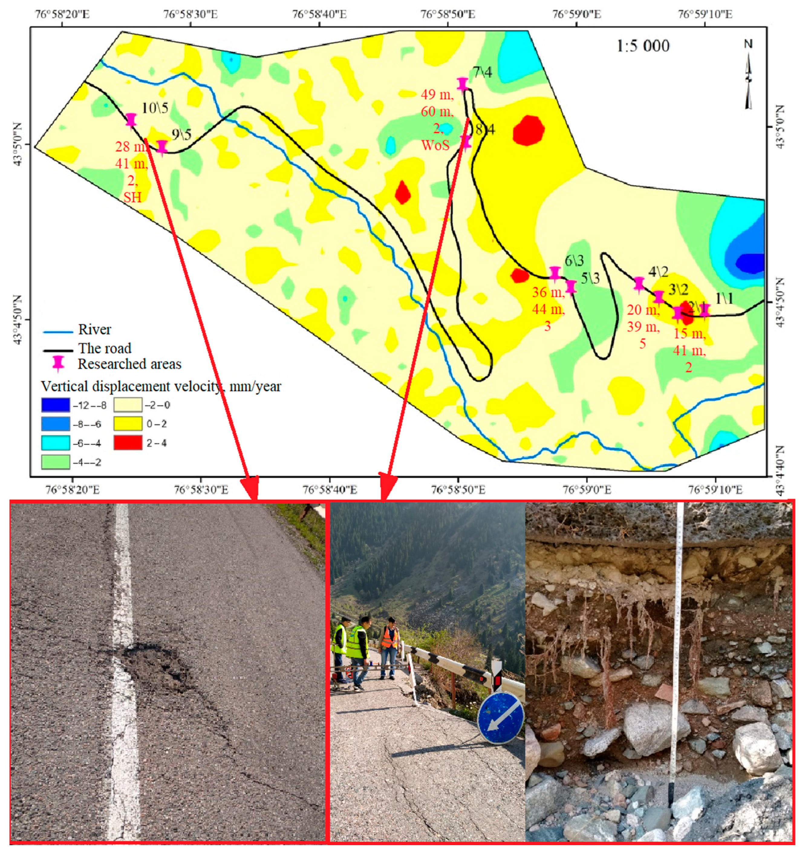
4.1. Road’s Deformation Data
4.2. Factual Meteorological Data
- Horizontal visibility at a 2 m level above the Earth’s surface, m;
- Natural phenomena names;
- Natural phenomena amount, mm;
- Basic cloudiness, %;
- Low level cloudiness (lower than 2000 m), %;
- Air temperature, °C;
- Air humidity, %;
- Rainfall, mm;
- Snow cover, cm.
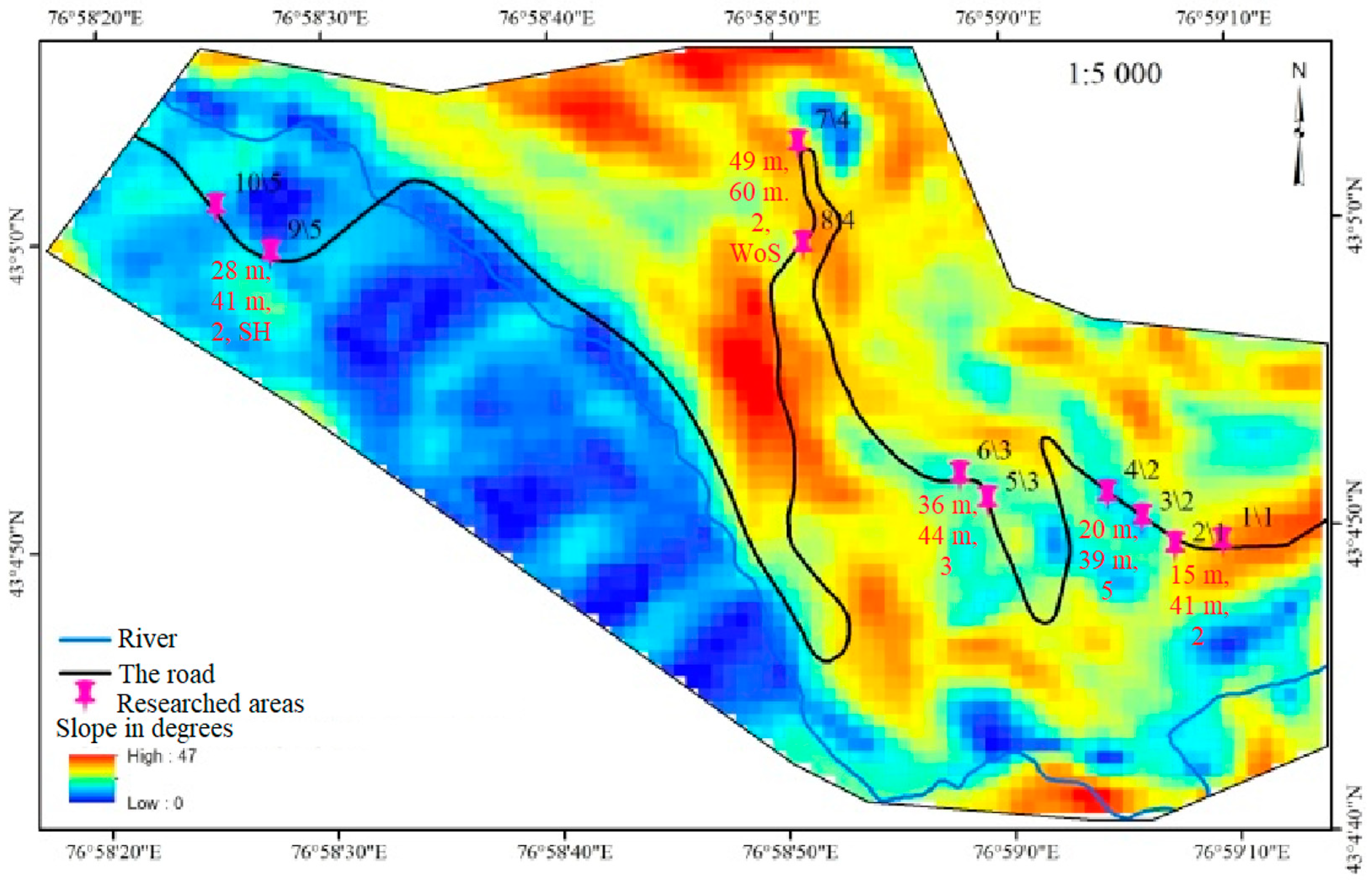
4.3. Correlation between Landscape and Road Deformation Data
- Total length of transversal cracks;
- Total length of longitudinal cracks;
- Essential destruction (SH—small holes, WoS—washed out slope).
- The first testing section is negatively affected by high vertical displacement velocity, high slope values, and solar radiation; its aspect is average; and its topographic wetness index is very low;
- The second testing section of the road is negatively affected by a moderate parallel difference of vertical displacement velocities and a high aspect and solar radiation, but the slope value and topographic wetness index are average;
- The third testing section of the road is negatively affected by a moderate parallel difference of vertical displacement velocities and the highest aspect, but the slope value, topographic wetness index, and solar radiation are average;
- The fourth testing section of the road is negatively affected by a high perpendicular difference of vertical displacement velocities, a high slope, a relatively high dissection index value, a high topographic wetness index, the highest aspect, and snow-melting, but its solar radiation is mixed;
- The fifth testing section of the road is negatively affected by a high topographic wetness index, SAVI, and snow melting, but its vertical displacement velocity and slope values are average and its dissection index, aspect, and solar radiation are very low.
5. Conclusions
Author Contributions
Funding
Data Availability Statement
Conflicts of Interest
References
- Gkyrtis, K.; Plati, C.; Loizos, A. Mechanistic Analysis of Asphalt Pavements in Support of Pavement Preservation Decision-Making. Infrastructures 2022, 7, 61. [Google Scholar] [CrossRef]
- Mičechová, L.; Mikolaj, J.; Šedivý, Š. New knowledge in the field of the diagnostic and evaluation of selected pavement parameters. Transp. Res. Procedia 2019, 40, 373–380. [Google Scholar] [CrossRef]
- Staniek, M.; Czech, P. Self-correcting Neural network in road pavement diagnostics. Autom. Constr. 2018, 96, 75–87. [Google Scholar] [CrossRef]
- Kheirati, A.; Golroo, A. Low-cost infrared-based pavement roughness data acquisition for low volume roads. Autom. Constr. 2020, 119, 103363. [Google Scholar] [CrossRef]
- Ďurinová, M.; Mikolaj, J. Definition of pavement performance models as a result of experimental measurements. Transp. Res. Procedia 2019, 40, 201–208. [Google Scholar] [CrossRef]
- Oreto, C.; Massotti, L.; Biancardo, S.A.; Veropalumbo, R.; Viscione, N.; Russo, F. BIM-Based Pavement Management Tool for Scheduling Urban Road Maintenance. Infrastructures 2021, 6, 148. [Google Scholar] [CrossRef]
- Braunfelds, J.; Senkans, U.; Skels, P.; Janeliukstis, R.; Porins, J.; Spolitis, S.; Bobrovs, V. Road Pavement Structural Health Monitoring by Embedded Fiber-Bragg-Grating-Based Optical Sensors. Sensors 2022, 22, 4581. [Google Scholar] [CrossRef]
- Al-Mansour, A.I.; Al-Qaili, A.H. An Application of Android Sensors and Google Earth in Pavement Maintenance Management Systems for Developing Countries. Appl. Sci. 2022, 12, 5636. [Google Scholar] [CrossRef]
- Zhantayev, Z.; Kairanbayeva, A.; Kiyalbayev, A.; Nurpeissova, G.; Panyukova, D. Data collection for intellectual forecasting: Metthods and results. News Natl. Acad. Sci. Repub. Kazakhstan. Ser. Phys.-Math. 2021, 4, 108–117. [Google Scholar] [CrossRef]
- Steger, S.; Mair, V.; Kofler, C.; Pittore, M.; Zebisch, M.; Schneiderbauer, S. Correlation does not imply geomorphic causation in data-driven landslide susceptibility modelling—Benefits of exploring landslide data collection effects. Sci. Total Environ. 2021, 776, 145935. [Google Scholar] [CrossRef]
- Intrieri, E.; Carlà, T.; Gigli, G. Forecasting the time of failure of landslides at slope-scale: A literature review. Earth-Sci. Rev. 2019, 193, 333–349. [Google Scholar] [CrossRef]
- Chikalamo, E.E.; Mavrouli, O.C.; Ettema, J.; van Westen, C.J.; Muntohar, A.S.; Mustofa, A. Satellite-derived rainfall thresholds for landslide early warning in Bogowonto Catchment, Central Java, Indonesia. Int. J. Appl. Earth Obs. Geoinf. 2020, 89, 102093. [Google Scholar] [CrossRef]
- Li, M.; Zhang, L.; Ding, C.; Li, W.; Luo, H.; Liao, M.; Xu, Q. Retrieval of historical surface displacements of the Baige landslide from time-series SAR observations for retrospective analysis of the collapse event. Remote Sens. Environ. 2020, 240, 111695. [Google Scholar] [CrossRef]
- Mondini, A.C.; Guzzetti, F.; Chang, K.-T.; Monserrat, O.; Martha, T.R.; Manconi, A. Landslide failures detection and mapping using Synthetic Aperture Radar: Past, present and future. Earth-Sci. Rev. 2021, 216, 103574. [Google Scholar] [CrossRef]
- Bondur, V.; Chimitdorzhiev, T.; Dmitriev, A.; Dagurov, P. Fusion of SAR Interferometry and Polarimetry Methods for Landslide Reactivation Study, the Bureya River (Russia) Event Case Study. Remote Sens. 2021, 13, 5136. [Google Scholar] [CrossRef]
- Teshebaeva, K.; Roessner, S.; Echtler, H.; Motagh, M.; Wetzel, H.-U.; Molodbekov, B. ALOS/PALSAR InSAR Time-Series Analysis for Detecting Very Slow-Moving Landslides in Southern Kyrgyzstan. Remote Sens. 2015, 7, 8973–8994. [Google Scholar] [CrossRef] [Green Version]
- Pfurtscheller, C.; Genovese, E. The Felbertauern landslide of 2013 in Austria: Impact on transport networks, regional economy and policy decisions. Case Stud. Transp. Policy 2019, 7, 643–654. [Google Scholar] [CrossRef]
- Zhang, Q.; Yu, H.; Li, Z.; Zhang, G.; Ma, D.T. Assessing potential likelihood and impacts of landslides on transportation network vulnerability. Transp. Res. Part D Transp. Environ. 2020, 82, 102304. [Google Scholar] [CrossRef]
- Leonardi, G.; Palamara, R.; Suraci, F. A fuzzy methodology to evaluate the landslide risk in road lifelines. Transp. Res. Procedia 2020, 45, 732–739. [Google Scholar] [CrossRef]
- Sarychikhina, O.; Palacios, D.G.; Argote, L.A.D.; Ortega, A.-G. Application of satellite SAR interferometry for the detection and monitoring of landslides along the Tijuana—Ensenada Scenic Highway, Baja California, Mexico. J. S. Am. Earth Sci. 2021, 107, 103030. [Google Scholar] [CrossRef]
- Lee, C.-F.; Huang, W.-K.; Chang, Y.-L.; Chi, S.-Y.; Liao, W.-C. Regional landslide susceptibility assessment using multi-stage remote sensing data along the coastal range highway in northeastern Taiwan. Geomorphology 2018, 300, 113–127. [Google Scholar] [CrossRef]
- Nappo, N.; Peduto, D.; Mavrouli, O.; van Westen, C.J.; Gullà, G. Slow-moving landslides interacting with the road network: Analysis of damage using ancillary data, in situ surveys and multi-source monitoring data. Eng. Geol. 2019, 260, 105244. [Google Scholar] [CrossRef]
- Official Website of the President of the Republic of Kazakhstan. Available online: https://www.akorda.kz/ru/republic_of_kazakhstan/kazakhstan (accessed on 1 September 2022).
- Central Asian Countries Geoportal. Available online: https://cac-geoportal.org/ (accessed on 3 September 2022).
- Kazakhstan Climate Zone, Weather by Month and Historical Data. Available online: https://tcktcktck.org/kazakhstan (accessed on 18 November 2022).
- Agency for Strategic Planning and Reforms of the Republic of Kazakhstan Bureau of National Statistics. Express Information. Available online: https://stat.gov.kz/official/industry/61/statistic/6 (accessed on 3 September 2022).
- Automobile Road’s Length. Available online: https://stat.gov.kz/api/getFile/?docId=ESTAT099963&lang=ru (accessed on 29 August 2022).
- Pantuso, A.; Loprencipe, G.; Bonin, G.; Teltayev, B.B. Analysis of Pavement Condition Survey Data for Effective Implementation of a Network Level Pavement Management Program for Kazakhstan. Sustainability 2019, 11, 901. [Google Scholar] [CrossRef] [Green Version]
- Bonin, G.; Folino, N.; Loprencipe, G.; Oliverio Rossi, G.; Polizzotti, S.; Teltayev, B. Development of a Road Asset Management System in Kazakhstan. In Proceedings of the TIS 2017 International Congress on Transport Infrastructure and Systems, Rome, Italy, 10–12 April 2017; pp. 10–12. [Google Scholar]
- PR RK 218-27-2014. Governmental Instruction for Diagnostics and Assessment of Traffic Operating Conditions of the Automobile Roads. (ΠP PK 218-27-2014). Available online: https://online.zakon.kz/Document/?doc_id=37657859&pos=1;-16#pos=1;-16 (accessed on 8 November 2022).
- ST RK 1219-2017. National Standard of the Republic of Kazakhstan for Automobile Roads and Airdromes “Methods of Measurement of Unevenness in Beddings and Covers” (CT PK 1219-2003). Available online: https://online.zakon.kz/Document/?doc_id=35447297&pos=3;-109#pos=3;-109 (accessed on 8 November 2022).
- Badeli, S.; Carter, A.; Doré, G. Effect of laboratory compaction on the viscoelastic characteristics of an asphalt mix before and after rapid freeze-Thaw cycles. Cold Reg. Sci. Technol. 2018, 146, 98–109. [Google Scholar] [CrossRef]
- ud Din, I.M.; Mir, M.S.; Farooq, M.A. Effect of Freeze-Thaw Cycles on the Properties of Asphalt Pavements in Cold Regions: A Review. Transp. Res. Procedia 2020, 48, 3634–3641. [Google Scholar] [CrossRef]
- Teltayev, B.B.O.; Rossi, C.; Izmailova, G.G.; Amirbayev, E.D. Effect of Freeze-Thaw Cycles on Mechanical Characteristics of Bitumens and Stone Mastic Asphalts. Appl. Sci. 2019, 9, 458. [Google Scholar] [CrossRef] [Green Version]
- Cao, H.; Chen, T.; Zhu, H.; Ren, H. Influence of Frequent Freeze-Thaw Cycles on Performance of Asphalt Pavement in High-Cold and High-Altitude Areas. Coatings 2022, 12, 752. [Google Scholar] [CrossRef]
- Capayova, S.; Cihlarova, D.; Mondschein, P. Effect of Winter Road Maintenance on the Asphalt Road Surface—Experience in Slovakia and the Czech Republic. Materials 2022, 15, 5618. [Google Scholar] [CrossRef]
- Cong, L.; Yang, F.; Guo, G.; Ren, M.; Shi, J.; Tan, L. The use of polyurethane for asphalt pavement engineering applications: A state-of-the-art review. Constr. Build. Mater. 2019, 225, 1012–1025. [Google Scholar] [CrossRef]
- Guo, X.; Hao, P. Using a Random Forest Model to Predict the Location of Potential Damage on Asphalt Pavement. Appl. Sci. 2021, 11, 10396. [Google Scholar] [CrossRef]
- Yang, S.L.; Baek, C.; Park, H.B. Effect of Aging and Moisture Damage on Fatigue Cracking Properties in Asphalt Mixtures. Appl. Sci. 2021, 11, 10543. [Google Scholar] [CrossRef]
- Dou, J.; Yunus, A.P.; Bui, D.T.; Merghadi, A.; Sahana, M.; Zhu, Z.; Chen, C.W.; Han, Z.; Pham, B.T. Improved landslide assessment using support vector machine with bagging, boosting, and stacking ensemble machine learning framework in a mountainous watershed, Japan. Landslides 2020, 17, 641–658. [Google Scholar] [CrossRef]
- Chen, H.-E.; Chiu, Y.-Y.; Tsai, T.-L.; Yang, J.-C. Effect of Rainfall, Runoff and Infiltration Processes on the Stability of Footslopes. Water 2020, 12, 1229. [Google Scholar] [CrossRef]
- Ivanov, V.; Arosio, D.; Tresoldi, G.; Hojat, A.; Zanzi, L.; Papini, M.; Longoni, L. Investigation on the Role of Water for the Stability of Shallow Landslides—Insights from Experimental Tests. Water 2020, 12, 1203. [Google Scholar] [CrossRef] [Green Version]
- Kirschbaum, D.; Stanley, T. Satellite-based assessment of rainfall-triggered and slide hazard for situational awareness. Earths Future 2018, 6, 505–523. [Google Scholar] [CrossRef]
- Uemoto, J.; Moriyama, T.; Nadai, A.; Kojima, S.; Umehara, T. Landslide detection based on height and amplitude differences using pre- and post-event airborne X-band SAR data. Nat. Hazards 2019, 95, 485–503. [Google Scholar] [CrossRef] [Green Version]
- Zhantayev, Z.; Talgarbayeva, D.; Kairanbayeva, A.; Panyukova, D.; Turekulova, K. Complex processing of earth remote sensing data for prediction of landslide processes on roads in mountain area. News Natl. Acad. Sci. Repub. Kazakhstan. Ser. Geol. Tech. Sci. 2022, 3, 181–197. [Google Scholar] [CrossRef]


| Climatic Zone | Fallouts | January | July | Details | |||
|---|---|---|---|---|---|---|---|
| Annual Number, mm | In Warm Period, % | Annual Temp., °C | Extreme Values, °C | Annual Temp., °C | Extreme Values, °C | ||
| Forest steppe | 320–360 | 80 | −17 | −(42–48) | 20 | 41 | Winter is long and cold, late spring and early fall have windchills, winter temperature rises up to +5 °C. |
| Steppe | 230–340 | 65–80 | −(15–19) | −(42–54) | 19–23 | 40–42 | Percent of winter fallouts up to 23–27% of the annual value, potential strong winds and snow windrows, 20–80 days of dust storms, long and hot summer. |
| Semi-desert | 134–330 | 55–70 | −(10–20) | −(37–50) | 21–25 | 40–45 | High frequency of atmospheric drought and drought wind weather. |
| Desert | 100–200 | 46–60 | −(5–15) | - | - | - | The soil surface can heat up to 70 °C in the daytime and cool to 0 °C at night. |
| Number of the Road km | Road Width, m | Score According to [30] | Details |
|---|---|---|---|
| 1 | 9.5 | I/1 | No deformation registered. |
| 2 | 9.5 | I/1 | No deformation registered. |
| 3 | 9.5 | I/1 | No deformation registered. |
| 4 | 9.5 | I/1 | No deformation registered. |
| 5 | 8.0 | I/1 | No deformation registered. |
| 6 | 8.0 | I/1 | No deformation registered. |
| 7 | 8.0 | I/1 | No deformation registered. |
| 8 | 8.0 | I/1 | No deformation registered. |
| 9 | 7.5 | I/3 | Transverse cracks and unevenness. |
| 10 | 7.5 | I/2–3 | Transverse cracks and unevenness. |
| 11 | 7.5 | I/2–3 | Transverse cracks and unevenness. |
| 12 | 7.5 | I/3–4 | Transverse cracks and unevenness. |
| 13 | 7.5 | I/4 | Transverse cracks and unevenness. |
| 14 | – | – | Construction work. No traffic. |
| 15 | – | – | Construction work. No traffic. |
| 16 | – | – | Construction work. No traffic. |
| 17 | 7.2 | I/1–2 | New roadbed. Some transverse cracks at 2–3 m intervals |
| 18 | 7.2 | I/2 | New roadbed. Some transverse cracks at 2–3 m intervals |
| 19 | 7.2 | I/4 | Clear longitudinal and transverse cracks. Occasional crack network. Washed out road slope (WoS). |
| 20 | 7.2 | I/4 | Clear longitudinal and transverse cracks. Occasional crack network. |
| 21 | 7.2 | II | Clear longitudinal and transverse cracks. Occasional crack network. |
| Testing Section | Transversal Crack by Length | Longitudinal Crack, m | Crack Network | Details | ||||||||
|---|---|---|---|---|---|---|---|---|---|---|---|---|
| 0–1 m | 1–2 m | 2–3 m | 3–4 m | 4–5 m | Total Length, m | On a Left Side | In a Center | On a Right Side | Total Length, m | |||
| 1/1–2/1 | 6 | 3 | 1 | - | - | 15 | ∑11.5 | ∑16.9 | ∑12.1 | 41 | 2 | - |
| 3/2–4/2 | 8 | 3 | 2 | - | - | 20 | ∑8 | ∑17.04 | ∑13.9 | 39 | 5 | - |
| 5/3–6/3 | 7 | 6 | 3 | 2 | - | 36 | ∑17.8 | ∑19.25 | ∑7.4 | 44 | 3 | - |
| 7/4–8/4 | 11 | 6 | 3 | 3 | 1 | 49 | ∑34.8 | ∑3.3 | ∑22.2 | 60 | 2 | Washed out road slope (WoS) |
| 9/5–10/5 | 5 | 4 | 2 | 1 | 1 | 28 | ∑6.8 | ∑18.1 | ∑15.6 | 41 | 2 | Small holes (SH) |
| Year | Extremely High Temperature (>30 °C), Number of 3 h Periods | Extremely Low Temperature (<−15 °C), Number of 3 h Periods | Freezing and Thawing Cycles, Number | Air Humidity (Min–Max), % | Highly Intensive Rainfall Values (More Than 30 mm un 3 h), Number of Periods | Rainfall/Snow Cover Maximum Value, mm/cm |
|---|---|---|---|---|---|---|
| 2016 | 62 | 1 | 102 | 0–100 | 10 | 43/42 |
| 2017 | 130 | 0 | 151 | 0–100 | 4 | 701/598 |
| 2018 | 107 | 60 | 93 | 0–100 | 0 | 26/25 |
| 2019 | 133 | 1 | 133 | 13–100 | 2 | 45/33 |
| 2020 | 76 | 0 | 105 | 0–100 | 3 | 320/598 |
| First 3 month of 2021 | 0 | 11 | 63 | 16–96 | 0 | 21/23 |
| Testing Section | Total Length of Transversal Crack, m/Total Length of Longitudinal Crack, m/Crack Network, Number/Details | Vertical Displacement Velocity | Slope Exposure | Dissections | Topographic Wetness Index | Aspect | Solar Radiation | Vegetation Index SAVI | Snow-Melting |
|---|---|---|---|---|---|---|---|---|---|
| 1/1–2/1 | 15/41/2 | ++ 1 | ++ | - | -- | - | ++ | - | - |
| 3/2–4/2 | 20/39/5 | ± | - | - | - | + | ++ | -- | - |
| 5/3–6/3 | 36/44/3 | ± | - | - | - | ++ | - | -- | - |
| 7/4–8/4 | 49/60/2/ Washed out road slope | -+ | ++ | + | ++ | ++ | ± | - | +++ |
| 9/5–10/5 | 28/41/2/Small holes | - | - | -- | ++ | -- | -- | ++ | ++ |
| Other parts of road | - | + | ++ | +++ | ++ | -- | ++ | ++ | +++ |
Publisher’s Note: MDPI stays neutral with regard to jurisdictional claims in published maps and institutional affiliations. |
© 2022 by the authors. Licensee MDPI, Basel, Switzerland. This article is an open access article distributed under the terms and conditions of the Creative Commons Attribution (CC BY) license (https://creativecommons.org/licenses/by/4.0/).
Share and Cite
Kairanbayeva, A.; Nurpeissova, G.; Zhantayev, Z.; Shults, R.; Panyukova, D.; Kiyalbay, S.; Panyukov, K. Impact of Landscape Factors on Automobile Road Deformation Patterns—A Case Study of the Almaty Mountain Road. Sustainability 2022, 14, 15466. https://doi.org/10.3390/su142215466
Kairanbayeva A, Nurpeissova G, Zhantayev Z, Shults R, Panyukova D, Kiyalbay S, Panyukov K. Impact of Landscape Factors on Automobile Road Deformation Patterns—A Case Study of the Almaty Mountain Road. Sustainability. 2022; 14(22):15466. https://doi.org/10.3390/su142215466
Chicago/Turabian StyleKairanbayeva, Ainur, Gulnara Nurpeissova, Zhumabek Zhantayev, Roman Shults, Dina Panyukova, Saniya Kiyalbay, and Kerey Panyukov. 2022. "Impact of Landscape Factors on Automobile Road Deformation Patterns—A Case Study of the Almaty Mountain Road" Sustainability 14, no. 22: 15466. https://doi.org/10.3390/su142215466