Smart Modelling of a Sustainable Biological Wastewater Treatment Technologies: A Critical Review

Abstract

One of the most essential operational difficulties that water companies face today is the capacity to manage their water treatment process daily. Companies are looking for long-term solutions to predict how their treatment methods may be enhanced as they face growing competition. Many models for biological growth rate control, such as the Monod and Contois models, have been suggested in the literature. This review further emphasized that the Contois model is the best and is more suited to predicting the performance of biological growth rate than the other applicable models with a high correlation coefficient. Furthermore, the most well-known models for optimizing and predicting the wastewater treatment process are response surface methodology (RSM) and artificial neural networks (ANN). Based on this review, the ANN is the best model for wastewater treatment with high accuracy in biological wastewater treatment. Furthermore, the present paper conducts a bibliometric analysis using VOSviewer to assess research performance and perform a scientific mapping of the most relevant literature in the field. A bibliometric study of the most recent publications in the SCOPUS database between 2018 and 2022 is performed to assess the top ten countries around the world in the publishing of employing these four models for wastewater treatment. Therefore, major contributors in the field include India, France, Iran, and China. Consequently, in this research, we propose a sustainable wastewater treatment model that uses the Contois model and the ANN model to save time and effort. This approach may be helpful in the design and operation of clean water treatment operations, as well as a tool for improving day-to-day performance management.

1. Introduction

Sustainable urban water systems need the supply of public drinking water and sanitation services and the promotion of balanced environmental, economic, and social health in communities today and in the future. Many countries are finding it difficult to solve population growth, water scarcity, climate change, and environmental concerns [1]. In most instances, surface freshwater is subject to pollution and contamination by pathogenic organisms and cannot be considered safe without treatment [2]. However, most urban water systems in developed countries can now supply water to urban areas and meet the sanitation demand through a central controller [3]. Furthermore, water purification is the primary focus of the urban system. In approximately 4000 BC civilizations for highly old processes such as water boiling, sand, and gravel filtration, and straining were discovered in ancient India and Greece. Since 1500 BC, the Egyptians have used carbonized wood as a medical adsorbent and purifier [4]. Between such water treatments, sedimentation was the major driving factor. The processes of bacterial microorganisms used in membrane bioreactors for wastewater treatment were not well explored. Consequently, finding the best mathematical modeling for wastewater treatment in membrane bioreactors is extremely crucial.

Over the years, different approaches have been developed to extract metal elements from wastewater by prioritizing simple, efficient, and cost-effective techniques as a fundamental concept [5]. The biological treatment of wastewater is a natural method where microorganisms break down organic or inorganic wastes [6,7,8,9]. It is used worldwide to reduce the quantity of polluted wastewater generated by industrial and other sources. Multi-stage biological wastewater treatment includes primary and secondary wastewater treatment as shown in Figure 1. Particle solids are mostly removed by sedimentation during the initial treatment. The secondary treatment follows, which involves the removal of substrates (suspended organic solids and organic dissolving chemicals) from wastewater by microorganisms in the form of activated sludge. Microorganisms are suspended in wastewater during the activated sludge procedure, and this mixture is known as “mixed liquor”. Two phases typically take the secondary treatment procedure. In the first phase, bacteria break down organic contaminants to support their life activities, including energy production, reproduction, digesting, and motion, in an aerated biological reactor.

The liquid remaining within the clarifier is piped into disinfection units and released into water for further treatment (known as ‘tertiary treatment’). The design of the sludge procedures addresses two key issues linked to sludge treatment. The amounts of suspended solids in the mixed liquor are generally referred to as MLSS. The biochemical oxygen demand (BOD) or the chemical request for oxygen (COD) shows how wastewater is laden with organic products. The microbial development that occurred by the utilization of nutrients in wastewater by microorganisms may be considered to describe the relationship between the concentration of micro-organs and the substrate. The concentration levels of the substrate and micro-organisms in the bioreactor rely on microbial growth, which depends on the kind of process and the operating method. Therefore, microbial development depends on several sorts of processes that might be easy or complicated to identify and manage [10]. A variety of membrane bioreactors are available, such as a membrane biofouling of a membrane bioreactor [11], Step-Aerating MBRs (membrane bioreactor) [12], and Pilot-Scale MBRs [13]. They are usually classed as open or closed systems. The system flows continuously for an open system. In a closed system, biomass growth is lowered with time, ultimately reaching zero, the unavoidable consequence when nutrients are insufficient to support growth [7,14].

Our models (Monod model, Contois models, response surface methodology (RSM), and artificial neural networks (ANN)) explore the secondary treatment of wastewater in a continuous flow reactor. However, we presume that the substrate or microorganism reactor concentrations are correctly mixed, which means that the substrate or microbe reactor concentrations are identical to the reactor.

As a result, there is growing interest in mathematical models that may be used to propose techniques to minimize the volume and mass of excessive pollutants as part of biological wastewater treatment techniques. Consequently, in this review, we represent mathematical models of Monod, Contois, response surface methodology (RSM), and artificial neural networks (ANN) models for water treatment processes in bioreactors by taking into account a single substrate concentration absorbed by a single microbe species and describing the reaction rate. The Monod and Contois kinetics models are used in this study to describe the growth rate of microorganisms for clean water treatment processes mathematically. The major objective is to propose the best methods that water companies may employ to forecast the performance of their water treatment processes, allowing for better management of scientific measurement errors. Furthermore, most modeling work in the water industry is response surface methodology (RSM) and artificial neural networks (ANN) models. Smart models are required to explain, forecast, and regulate the complex interactions between the many stages of the treatment process, a widely recognized principle in the process industry but have yet to be adopted by the water treatment sector. Using first-principles parametric modeling, this article builds a conceptual understanding of clean water treatment systems.

The main purpose of this study is to find the best model of a whole biological water treatment process, which will allow for a better understanding of how changes in one processing unit affect the whole treatment process. This is, to the best of our knowledge, the first review addressing these four wastewater treatment models. To assess the top ten countries around the world applying these models in wastewater treatment, a bibliometric study of the most current articles between 2018 and 2022 is conducted. The primary goal of bibliometric indicators is to effectively represent important aspects of scientific issues. In the present study, the most prominent nations were identified using bibliometric markers, such as co-authorship analysis. The study makes use of Scopus, the biggest database for scientific research papers. Scopus has information on all active research topics and is thus employed in this research. In addition, OSViewer (version 1.6.18) is employed in this work. VOSviewer has been developed by Nees Jan van Eck and Ludo Waltman at Leiden University’s Center for Science and Technology Studies (CWTS) in the Netherlands.

2. Bach Model

2.1. Anaerobic and Aerobic Wastewater Treatment

Organic matter is largely removed from wastewater by two biological processes: anaerobic and aerobic. The most important distinctions between aerobic and anaerobic processes are shown in

Table 1. The most important distinctions between aerobic and anaerobic processes [21], with permission from Elsevier.

Parameter	Aerobic Treatment	Anaerobic Treatment
Organic removal efficiency	High	High
Effluent quality	Excellent	Moderate to poor
Organic loading rate	Moderate	High
Sludge production	High	Low
Nutrient requirement	High	Low
Alkalinity requirement	Low	High for certain industrial waste
Energy requirement	High	Low to moderate
Temperature sensitivity	Low	High
Start-up time	2–4 weeks	2–4 months
Odor	Less opportunity for odors	Potential odor problems
Bioenergy and nutrient recovery	No	Yes

. They were effectively used to treat waste fluids from different types of household and industrial wastes. For bacteria to break down organic materials, the anaerobic process requires no oxygen, whereas oxygen is needed in the aerobic process. The energy it needs is one of the biggest disadvantages of the aerobic method [15].

Consequently, anaerobic methods are usually preferred for the treatment of highly organic waste effluent [16]. The advantages of anaerobic treatments include no aeration needs, very high biological loading speed, sparse area, low nutritional requirements, excellent stability, enhanced energy generation, and low cost [17]. On the other hand, the major disadvantages of the anaerobic process treatment are the environmental sensitivities, installation, and monitoring of a system group for safe hand heating of the tank, reducing the temperature control range, and the accumulation of heavy metals and sludge pollutants. The anaerobic process has three serial phases of biological reaction. These are the phase of hydrolysis, acidgenesis, and methanogenesis, which transform organic materials into methane (CH₄) and carbon dioxide (CO₂) [18]. In the first phase, bacterial hydrolysis breaks up insoluble organic polymers into the soluble substrate that these bacteria may use. In the second stage, acidic bacteria transform the materials into carbohydrates, hydrogen, and other materials, such as CO₂, H₂, NH_3, and organic acids, such as acetates, propionates, and butyrates from the first stage. In the third step, methanogenic bacteria transform the products from the second stage into methane [19]. The mechanisms are typically dependent on several bacterial species in all three phases [20]. The kinetics connected with the three phases of anaerobic digestion has been increasingly concerning over the past few years. Consequently, differences in the process of anaerobic digestion have been extensively characterized using models that reflect the process.

2.2. Microbial Growth

The number of cells and the mass of the bacteria as a result of the cell division is increased by microbial growth. Microbial growth may be affected by several variables, which are described as intracellular and extracellular. The external environmental variables affecting cells include pH, temperature, the concentration of oxygen, water, and food. At the same time, the internal structure, metabolic processes, and genetic material of the cell are intracellular factors. Biomass growth in a culture demands that microorganisms have the right environment to live in and develop. It must meet numerous requirements, including viable inoculum, an energy supply, nutrition, lack of growth-preventing inhibitors, and appropriate physicochemical parameters. It is crucial to understand how the concentrations of typical system components, i.e., cells, substrate, products, and by-products, fluctuate over time in investigating the kinetic behavior of such a system. The microbial growth research in terms of several variables (different growth parameters) is helpful for many applications and is needed to anticipate and manage the system’s behavior. These criteria of growth are developed to explain the development of easy and difficult cultures. Specific growth, growth yield, metabolism for the consumption of the substrates, and the creation of product and maximal biomass are thus included in these criteria. Figure 2 shows the four major phases of the growth curve of the bacteria. The lag phase was the time when the individual bacteria were growing and adjusting to their new surroundings. However, the cells were not inactive and merely altered very slightly as they gathered nutrients in preparation for cell division [22].

2.3. Specific Growth Rate

If all the growth criteria are met, the concentration of biomass will rise exponentially with time, as the total rate of biomass change is proportional to the biomass mass as described in the following equation:

$$\frac{dx}{ dt}=\mathsf{\mu }x$$

(1)

where $x$ is the cell concentration (kg cell/m³), and the parameter $\mathsf{\mu }$ is called the specific growth rate by the unit of biomass. While the difference ($\frac{dx}{dt}$) is the rate of population increase, which indicates the rate of growth per unit of biomass and is referred to as the specific growth rate.

2.4. Growth Yield

The rates of production and consumption of energy and mass in the biological system may be assessed using the variable biological growth. The observed growth rate is quite useful in terms of modeling and characterizing such systems. The growth rate is described as the equation below:

$$Y_{x/s}=\frac{r_x}{r_s}$$

(2)

where $r_s$ is the consumed quantity and $r_x$ the biomass generated.

If the reaction rates are equivalent to those in batch systems, the growth rate is described as the following equation:

$$Y_{x/s}=-\frac{\frac{dx}{dt}}{\frac{ds}{dt}}=-\frac{dx}{ds}$$

(3)

The growth rate is determined for a continuous system as the following equation:

$$Y_{x/s}=-\frac{\Delta x}{\Delta s}=-\frac{x-x_0}{s-s_0}$$

(4)

where $x$ and $s$ are the concentrations corresponding to the culture’s growth, $x_0$ is the starting biomass and $s_0$ is the concentration of substrate. In order to represent this fact, the growth rate of $x$ and $s$ is marked by opposing indications. If the culture reaches its maximum biomass ($x_m$) and is close to zero, the growth yield is limited to a growth substrate that may be characterized as follows:

$$Y_{x/s}=\frac{x_m-x_0}{s_0}$$

(5)

The yield of growth is an essential metric since it reflects the organism’s nutrient requirements in terms of quantity. In certain bacterial cultures, when circumstances are kept constant the growth output is constant. However, it is deemed varied in other research [23].

2.5. Metabolic Quotient

The rate of an organism’s use of the substratum is the rate of substrate consumption. This rate is specified by the following equation:

$$q_{x }=-\frac{ds}{dt}$$

(6)

where q is known as the metabolic quotient and $x$ is the biomass.

$q_{x }$ must be consistent while the biomass content is constant, and the environmental factors are constant. A substrate uptake rate of the microbial cells can be determined by correlating growth yield with growth rate where $q_{x }$ is the substrate uptake rate and Y_X/S the growth yield. The growth yield is defined as the amount of grown cell per uptaken substrate amount. The growth yields of various kinds of cells have been reported. In this case, as the growth-limiting substrate, Y_X/S for most bacteria and yeast growing aerobically range by dry cell weight g⁻¹ substrate. The specific substrate uptake rate is:

$$\frac{ds}{dt}=\frac{\mathsf{\mu }x}{Y_{x/s}}$$

(7)

2.6. Effect of Substrate Concentration on Growth Rate

The growth rate of the microbe (and hence the concentration of the microorganism) is directly proportional to the substrate concentration typically eaten by the micro-organisms. However, the growth rate is practically unaffected by the level of substrates in some bacterial cultures, i.e., kinetics of zero order are available. If the consumption of the substrate is following the kinetics of enzymes, the metabolic quotient is:

$$\mathrm{q}=q_{max} \left(\frac{s}{k_s+s}\right)$$

(8)

where $q_{max}$ is the maximum saturation constant and $k_s$ the constant saturation equal to the constant Michaelis Menten [24].

When we make substitutions of:

$$\mathrm{q}=\frac{\mathsf{\mu }}{Y} \mathrm{and} q_{max}=\frac{\mathsf{\mu } max}{Y}$$

(9)

The equation is known as the Monod equation; the equation is as follows:

$$\mathsf{\mu }={\mathsf{\mu }}_{max} (\frac{s}{k_s+s})$$

(10)

3. Mathematical Model

Degradable solids, or substrates, break down into smaller soluble molecules. Microorganisms thrive on various substrates and create biomass. Several studies have found a relationship between biomass increase and substrate degradation. During the acid phase of anaerobic digestion, for example, substrate hydrolysis and fermentation, and biomass increase are examples of this. A continuous flow bioreactor’s condition may be described in terms of the variables that make up the microbe and the growth-limiting substrate. During the acid-phase digestion of municipal primary sludge, substrate degradation has also been explored using a variety of operational and environmental parameters such as hydraulic retention time (HRT), solids retention time (SRT), pH, and membrane bioreactor.

3.1. Monod Model

The Monod model depicts the link between the concentrations of microbiological organisms and the medium or substance on which the organisms survive [25,26]. As a result, the Monod model may be used to characterize bacterial culture development. The Monod model’s particular growth rate is:

$$\mu \left(S\right)=\frac{{\mu }_m S}{K_s+S}$$

(11)

where S is the concentration of biodegradable solids (hereinafter referred to as a substrate), Ks indicates the Monod constant or saturation constant (the most difficult parameter to get from testing), and m represents the maximal specific growth rate. The substrate concentration at which the specific growth rate is half that of the highest specific growth rate is called the half-maximum specific growth rate. The growth rate is assumed to be proportional to the number of nutrients available in this model. This results in a coupled system of two differential equations, one for microbe population and the other for nutrient concentration [27]. It is assumed that the reaction mixture has been correctly mixed. The Monod model for microorganism microbial development, in which bacteria and nutrients exist in water or a liquid phase and there is only one nutrient, is provided by [28]:

$$\frac{d}{dt}\left(C_i\right)=T_i\left(C_M,C_N\right)$$

(12)

where $M$ and $N$ indicate microorganisms (“small creatures such as mold, yeasts, and bacteria”), $C_i$ represents the mass concentration of reactant per unit volume of the liquid phase, and $T_i$ refers to the overall rate at which species $i$ is formed through reactions and sources. The Monod Equation (13) gives the rate of microbial growth as the following:

$$\mu \left(C_i\right)=\frac{{\mu }_m{C}_i}{K_s+C_i} , i=M, N$$

(13)

The final form of the governing system of differential equations, assuming that the microbial mortality rate is proportionate to the population size, is:

$$\frac{d{C}_M}{dt}=\frac{{\mu }_m{C}_N}{K_s+C_N}{C}_M-k_r{C}_M$$

(14)

$$\frac{d{C}_N}{dt}=-\frac{1}{Y} \frac{{\mu }_m{C}_N}{K_s+C_N} C_M$$

(15)

where $Y$ is the yield coefficient, and $k_r$ is the first-order endogenous decay rate. The development of species $C_M$ on the nutrients $C_N$ is represented by the first term on the right-hand side of the Equation (15). The second term on the right-hand side of Equation (15) represents the degradation of microorganisms. The loss of nutrients due to microbes consuming them is represented by the first term on the right-hand side of the Equation (15). The Monod model, still the most extensively used technique, is adaptable and robust enough to be explored quantitatively, numerically, and experimentally in environmental engineering processes. A continuous flow bioreactor and membrane reactor models were studied using the fundamental concept. When substrate ($S$) is devoured by biomass, which produces products (P, not illustrated), Equation (16) depicts the biochemistry of the biochemical process ($X_b$). Death causes the latter to create unspecified stuff (not visible) ($k_d$). The reactor discharges unused substrate, microorganisms, and the finished product. Unused substrate, microbes, and the product pass via the basic model’s schematic design, as illustrated below:

$$\mathrm{S} \stackrel{\mu \left(S\right)}{\to } X_b \stackrel{k_d}{\to }$$

(16)

Model Elaboration in Bioreactor

The basic approaches for mathematical modeling of the biological wastewater process were highlighted in this section, as illustrated in Figure 3. The model is based on the following hypotheses: the aeration tank is constantly stirred and mixed, no bio-reaction occurs in the settler, and only sludge is re-circulated in the aerobic biological reactor, oxygen and substrate concentrations are ignored along with the recirculation flow, and the exit flow rate from the aeration tank equals the sum of the exit flow rate from the separator and the flange flow rate.

The following parts cover a simplified system model for biological wastewater treatment. Two consecutive tanks, an air tank, and a settler are the most important in the model. Bacteria and other micro-organisms feed the inbound wastewaters in the aerated tank (also known as the aerobic biological reactor), which is released into the tank, and therefore reduces the degradation. The clarifier tank, also known as a settler, is a gravity sedimentation tank that separates the sludge from the clear remaining water. Part of the settled active sludge will be returned from the settler to the ventilation reactor to ensure an adequate level of the micro-organism (population) content in the aerobic reactor can be maintained to continue with the treatment of wastewater. As a result, excess active sludge from the biological wastewater treatment system is released (Figure 4).

There are four main equations for a model determination that seek to perform the procedure by isolating influences [29,30]:

(i) Equation associated with an active sludge balancing at the aeration tank level—the process of raising the sludge’s active mass:

$$\frac{dX\left(t\right)}{dt}=\mathsf{\mu }\left(t\right)X\left(t\right)-D\left(t\right)\left(1+r\right)X\left(t\right)+rD\left(t\right)X_r\left(t\right)$$

(17)

(ii) Equation associated with the substrate mass balance—the process of breakdown of organic molecules based on carbon:

$$\frac{dS\left(t\right)}{dt}=-\frac{\mathsf{\mu }\left(t\right)}{Y} X\left(t\right)-D\left(t\right)\left(1+r\right)S\left(t\right)+D\left(t\right)S_{in}$$

(18)

(iii) Equation connected to the mass balance of the water mass oxygen, the process of oxygen transfers by air provided in the water with special equipment: oxygen-consuming the biochemical breakdown of the organic matter:

$$\frac{d{D}_0\left(t\right)}{dt}=-K_0\frac{\mathsf{\mu }\left(t\right)}{Y}X\left(t\right)-D\left(t\right)\left(1+r\right)DO\left(t\right)+D\left(t\right)D{O}_{in}+\alpha W\left[D{O}_{mas}-DO\left(t\right)\right]$$

(19)

(iv) Equation associated with settling tank balance of the active sludge:

$$\frac{d{X}_r\left(t\right)}{dt}=D\left(t\right)\left(1+r\right)X\left(t\right)-D\left(t\right)\left(\beta +r \right)X_r\left(t\right)$$

(20)

The following notes have been applied to the above equations:

The ratio between the waste flow rate and the influent flow rate $(\beta$), the ratio between the re-circulated flow rate and the influent flow rate ($r$), aeration rate ($W$), model constant ($K_0$), oxygen transfer rate ($\alpha$), concentrations of dissolved oxygen and the substrate in the mass of the influent (Sin and DOin), biomass yield factor ($Y$), dilution rate (the ratio between the flow rate of the influent and the volume of the aeration tank) $D\left(t\right)$, recycled biomass $X_r\left(t\right)$, maximum amount of dissolved oxygen $D{O}_{mas}$, dissolved oxygen $DO\left(t\right)$, biomass $X\left(t\right)$, and substrate $S\left(t\right)$.

The biomass growth rate μ is a complex function affected by physical, chemical, and physiological factors. Various analytical regulations have been proposed for modeling this parameter. The best known is Monod law [31], however, in this instance, it is assumed that μ would rely on substrate concentration, dissolved oxygen concentration, and other kinetic parameters according to the Olsson model as follows [29]:

$$\mathsf{\mu }={\mathsf{\mu }}_{max} \frac{S\left(t\right)}{K_s+S\left(t\right)}+\frac{DO\left(t\right)}{K_{DO}+DO\left(t\right)}$$

(21)

where $K_{DO}$ refer to saturation constants, $S$ refers to the level of pollutant concentration, $K_s$ refer to the affinity constant, which expresses the degradation dependence, and ${\mathsf{\mu }}_{max}$refer to the maximum value of the specific growth rate.

3.2. The Theory of Contois (Modeling for Biological Treatment)

A key component of kinetic models for many biological processes is the rate at which a microbial population (X) expands, and the substrate (S) is consumed. In the past, scientists have often acted under the false assumption that the particular growth rate does not change with the number of organisms present [25,32]. Moreover, experimental results suggest that in certain systems, the substrate and microbial concentrations should be included in the specific growth rate model. Contois [33] established a similar concept of growth kinetics by presenting evidence from investigations of batch cultures developing under circumstances of nutrient constraint that the specific growth rate might also rely upon the microbe concentration. It can be shown that the Contois growth model consists of,

$$\mathsf{\mu }\left(S, X\right)={\mathsf{\mu }}_{max}+\left(\frac{S}{K_{s}X+S}\right)$$

(22)

where the microbe concentration ($X$) and substrate concentration ($S$) determine the specific growth rate $\mathsf{\mu }\left(S, X\right)$. Maximum specific growth rate and saturation constant, denoted by µmax and Ks, respectively. Under certain situations, their values remain unchanged.

According to the model developed by Contois, the growth rate $\mathsf{\mu }\left(S, X\right)$decreases as the concentration of microorganisms rises. The exponential growth rate is:

$$\mathrm{G}={\mathsf{\mu }}_{max}+\left(\frac{S}{K_{s}X+S}\right)$$

(23)

$$\mathrm{X}={\mathsf{\mu }}_{max}+\left(\frac{S/X}{K_s+S/X}\right)\times X$$

(24)

As the population density of bio-mass rises, the Contois model may be thought of as having two extreme situations. When this occurs, the Contois model for biomass or substrate concentration simplifies to first-order kinetics. As precisely as possible, these estimates are [34],

• Biomass development follows a first-order kinetics model.
• Substrate utilization kinetics are first order.

When the concentration of bio-mass is high, the Contois growth rate has been utilized as a surface-limiting model to explain the mass transfer restrictions owing to the restricted surface area [35,36]. Here, we express the rate of increase in detail as,

$$\mathsf{\mu }={\mathsf{\mu }}_{max}+\left(\frac{S/X}{K_s+S/X}\right)$$

(25)

3.2.1. The Kinetics of Inhibition and Growth in Contois

Inhibition of substrates is a crucial step in the breakdown of organic matter by microorganisms. Substrate inhibition is not accounted for in the Monod model. This modified variation of the Monod model, which Andrew developed by adding substrate inhibition, has found widespread use in the study of biological reactions. That is why adding substrate inhibition to the Contois model might considerably broaden the model’s usefulness. To do this, we must adapt the growth rate model in the following ways:

$$\mathsf{\mu }={\mathsf{\mu }}_{max}+\left(\frac{S}{K_{M}X+S+\frac{S^2}{K_1}}\right)$$

(26)

3.2.2. Microbiological Applications of the Contois Kinetics Model

There are cases when it is discovered that the Contois model provides a better match to experimental data than models that do not account for biomass concentration (such as the Monod model).

The causes of this phenomenon have been investigated by scientists from a wide range of disciplines. When the mass transfer is growth-limiting or enzyme kinetics are growth-limiting, the Contois model may be developed mechanistically based on saturation kinetics, as described by Fujimoto [37] and Characklis [38]. Furthermore, one of the most essential characteristics in the application of the Contois model is the presence of a local medium that is heterogeneous and that surrounds the cell, resulting in limited access to the substrate by the biomass [39,40]. The process by which the growth rate is determined was examined by Arditi and Ginzburg [41]. Predator-prey ratios were shown to be more relevant than prey alone when defining population growth-rate mechanisms. Other researchers have supplied further information [42,43,44] in favor of this concept.

3.2.3. Research Based on Models

This section provides a brief overview of the research on Contois kinetics-based reactor models. While the Monod expression has been the standard for describing microbial growth rate, some scientists have employed Contois kinetics to simulate growth dynamics in wastewater treatment systems [45,46,47,48].

Nelson, Balakrishnan, Sidhu, and Chen [46] pioneered the use of a Contois model to predict the growth rate in a single reactor with recycling. They demonstrated that the effluent concentration could be lowered to any value using a sufficiently long residence period. However, this is not the case for processes governed by Monod kinetics, where a limiting value exists for the concentration of the effluent [49].

Nelson and Holder [50] investigated the behavior of an N-reactant cascade without recycling and provided steady-state solutions along with a stability study.

Their goal was to find the optimum residence duration and number of tanks to reduce the effluent concentration. A significant reduction in effluent concentration was obtained by increasing the number of reactors in the reactor cascade in the vast majority of the situations evaluated. According to their findings, the substrate concentration that exits an N reactor cascade (Sn) decreases in value.

Many researchers have studied reactor dynamics with a linear yield coefficient and a specific growth rate consistent with the Contois model [47,51,52].

Nelson and Sidhu [23] studied the effects of a single and double reactor cascade using a continuously stirred reactor with good mixing. They looked at two scenarios assuming there was no mortality rate. In the first scenario, they determined the steady-state solutions and washed-out conditions for the model of a single reactor. Finally, they identified a range of values for the parameters that allowed the oscillation to maintain itself. It was also shown that periodic behavior is undesirable since the time-averaged effluent concentration is an increasing function of the residence duration.

In the second scenario, they assumed that the total residence time in the cascade would remain constant while they investigated how changing the residence time in the first reactor would affect the performance of the cascade as a whole. For the same amount of residence time, the cascade’s performance may fall short of that of a single reactor. On the other hand, the ideal performance of the cascade was consistently superior to that of the single reactor.

Nelson, Chen, and Sidhu [51] a membrane reactor where the microorganism mortality rate is not zero were further examined. They analyzed the model in the same way as in [23], examining at how the mortality rate influenced the performance of both a single reactor and a double reactor cascade

By extending Nelson and Sidhu [23], Ajbar, AlAhmad, and Ali [45] accounted for oxygen transport constraints. The performance of the reactor was accomplished by measuring process efficiency and productivity to identify the steady-state solutions and their stability. Reactor efficiency was up but productivity went down when the influent concentration was lowered.

As the oxygen transfer coefficient dropped, so did the reactor’s efficiency. It was determined that a yield coefficient that may vary is required to provide a periodic solution, but that this very slightly impacts reactor performance.

Two populations of microorganisms competed for the same substrate, each with a different yield coefficient, in a chemostat model studied by Ajbar [52]. The Contois model is used to predict the specific growth rates of both species. The analysis of this model revealed that the assumption of non-constant yield might result in intricate behaviors like chaotic behavior.

3.3. Response Surface Methodology (RSM))

The term “response surface methodology” (RSM) refers to a group of statistical and mathematical methods that may be used for the creation, enhancement, and optimization of various processes [53]. It provides an algebraic form for the polynomial equations that characterize the connection between independent variables and dependent measures. Initial work on RSM focused on simulating experimental responses [54,55], and subsequent work expanded the method to include numerical experiment modeling [56].

By using RSM for design optimization, we may cut down on the time and money spent on computationally intensive analytical techniques like the finite element method and computational fluid dynamics [57]. There is a lack of understanding about the nature of the connection between the independent factors and the outcome. Finding a good estimate of the real functional connection between dependent and independent variables is the ultimate aim of RSM. Low-order polynomials (often first or second) predominate, with second-order models typically being adequate for reflecting data and trends of more complicated models because of their adaptability and amenability to least-squares parameter estimation. When modeling with numerous polynomials of the second order, the typical governing equation looks like this:

$$\mathrm{Z}={\mathsf{\beta }}_0+{\mathsf{\beta }}_{\mathrm{i}}{\mathrm{x}}_{\mathrm{i}}+{\mathsf{\beta }}_{\mathrm{j}}{\mathrm{x}}_{\mathrm{j}}+{\mathsf{\beta }}_{\mathrm{ii}}{\mathrm{x}}_{\mathrm{i}}^2+{\mathsf{\beta }}_{\mathrm{ij}}{\mathrm{x}}_{\mathrm{j}}^2+{\mathsf{\beta }}_{\mathrm{ij}}{\mathrm{x}}_{\mathrm{i}}{\mathrm{x}}_{\mathrm{j}}$$

(27)

where

$Z$: Predicted response

${\beta }_0$: Constant Coefficient

${\beta }_i$, ${\beta }_j$: Linear Interaction Coefficient

${\beta }_{ii}$, ${\beta }_{ij}$: Quadratic Interaction Coefficients

$x_i$, $x_j$: Input Variables Influencing Predicted Response Z

Estimating regression coefficients is often done using the approach of least squares, as there is not enough plant data to apply ANN to make an acceptable system, the RSM model will be employed instead. The produced surrogate models will be compared to the detailed models both within and outside of the required range, between the low and high targets, to confirm their usage by assessing the accuracy of the model using parity plots.

3.4. Artificial Neutral Networks (ANN)

Through regression analysis, ANN models are constructed; these models are black boxes that provide results based on either experimental data or results from exact and computationally intensive models. By making close approximations of the functional connection between independent input variables and the continuous output or response variables, regression analysis allows for the prediction of the latter from the former [58]. Models of ANNs constructed from a large pool of data points tend to be more accurate than those constructed from a smaller pool of data points owing to a lack of information. Predicting output variables from relevant input variables using ANN models constructed with fewer data points is possible without giving specifics of the complicated processes [59,60], but ANN models constructed using approximation information may provide biased findings. Understanding the real underlying functional connection with variables, which is oared by sophisticated models, is more critical. Repeated simulations may provide more data points if precise mathematical models are not used. Regression analysis may estimate the behavior of the whole system with the help of smaller functions while yet maintaining the required precision [61,62,63].

Artificial neural networks (ANN) [64,65] and the response surface model (linear and multi-variable linear regression) [66,67] are the two most commonly used techniques for water quality modeling in the literature. The primary distinction between ANN and the other approach is that it generates mapping sequences between the input and output datasets. In order to forecast process outputs for data that was not used to train the network, the network must be “trained”, or mapped from inputs to outputs using past data. If not enough data is available for an ANN to benefit from its optimization, a linear regression model may be better adjusted regardless of the existing non-linearities.

Furthermore, experimental data were introduced; for training, testing, and validation process before the conversion of all data to normalized values (Xnorm), set in the range of 0.1 to 0.9 to avoid any scaling impact according to Equation below Xi represented the input or output data, whereas Xmin and Xmax were the minimum and maximum value of the data [7]:

$${\mathrm{X}}_{\mathrm{norm}}= 0.8 \times \left[\frac{{\mathrm{X}}_{\mathrm{i}}-{ \mathrm{X}}_{\min }}{{\mathrm{X}}_{\max }-{ \mathrm{X}}_{\min }}\right]+0.1$$

(28)

Artificial neural networks (ANN) were carried out in MATLAB 2017b via the function of net = newff (I, O, [7], ‘logsig’ ‘purelin’), where both the logistic and linear functions were obtained for the best activation signals for the network. They were expressed as (respectively) [8]:

$${\mathrm{f}}_1\left(\mathrm{x}\right)=\frac{1}{1+{ \mathrm{e}}^{-\mathrm{x}}}$$

(29)

$${\mathrm{f}}_2\left(\mathrm{x}\right)=\mathrm{ax}+\mathrm{b}$$

(30)

Inspired by the workings of the biological nervous system (biological neural networks), a mathematical model or algorithm known as an artificial neural network (ANN) has been created [68]. Simply stated, non-linear statistical data modeling methods like neural networks are used to describe intricate interdependencies between variables. During the training phase, ANNs may adjust their architecture in response to new input from the environment or from inside the network itself. Ultimately, via a learning process, the network acquires information, which is then stored in the links between the nodes of the network [69]. The approximation of functions is a common use of ANN, and they excel in situations when there is a large amount of training data available [70]. When given enough training data, ANNs can adequately describe multivariate systems with non-linear dynamics [71]. Figure 5 depicts a typical structure of the ANN model, the most common kind of ANN. Weighted connections connect the input layer, the hidden layer, and the output layer, and the biases of the nodes together reflect the system parameters [72]. The ANN takes in data at the input layer, processes it, and then passes the results on to the hidden layer. Information is further processed computationally at the hidden layer before being delivered to the output layer, which supplies information about the processing system. In a typical neural network, the input layer receives data from the training and validation sets, whereas the hidden and output layers get data directly from the nodes in the input layer. In the field of wastewater, ANN has been utilized to explain the biochemical reactions that take place throughout the biological treatment process [73,74].

4. Applications of the Mathematical Model

4.1. Application of the Monod Model in Wastewater Treatment

The influence of initial substrate concentration on growth rate is expressed as the following equation in the Modified Monod model [75]:

$$\mu \left(S\right)=\frac{{\mu }_{max}S}{K_s{S}_0+S}$$

(31)

where $S_0$ indicates the starting concentration of substrate.

Many processes, such as aerobic fermentation and the biological treatment of industrial wastewater and pollutants, use substrate inhibition when the substrate is hazardous to the microbe. The Monod model is a proportional increase in substrate concentration; the more substrate available, the faster the microorganisms reproduce [76]. The specific growth rate for systems susceptible to substrate inhibition is an increasing function at low substrate concentrations and a decreasing function at high substrate concentrations as the following:

$$\frac{d\mu }{ds}>0 if S<S_{cr}$$

(32)

$$\frac{d\mu }{ds}<0 if S>S_{cr}$$

(33)

where Scr is the value of the substrate concentration where the substrate inhibition is added, i.e., the point at which the specific growth rate changes from an increasing to a decreasing function of the substrate concentration [76].

The Contois model permits the biomass concentration to affect the specific growth rate as the following [75],

$$\mu \left(S, X\right)=\frac{{\mu }_{max}S}{K_{X}X+S}$$

(34)

The Contois kinetic constant is $K_X$ and the biomass concentration is X. Due to a growing barrier to substrate absorption, the specific growth rate in this model diminishes as the biomass grows.

In the acid phase of anaerobic digestion, a simple model for solubilization was given, with both hydrolysis and fermentation processes happening in sequence, as illustrated in Equation (2). Degradable particles (F) are hydrolyzed ($k_h$ into soluble substrates in the first step (S). The soluble substrates (S) are consumed (S) in the second step to yield acid phase products (P) and biomass (X). After that, the biomass decomposes (kd) into an unknown substance (U).

$$\mathrm{F} \stackrel{k_h}{\to } S \stackrel{\mu \left(s\right)}{\to } X \stackrel{k_d}{\to } U$$

(35)

$$\mathrm{F} \stackrel{k_h}{\to } S \stackrel{\mu \left(s\right)}{\to } P$$

(36)

In the acid phase model, Monod’s equation was utilized to represent the bacterial growth rate at constant temperature and pH. Hybrid differential evolution was used to estimate the parameters of the Monod model for recombinant fermentation [22]. The model profiles based on the starting glucose levels were found to be a good fit for the experimental data [22].

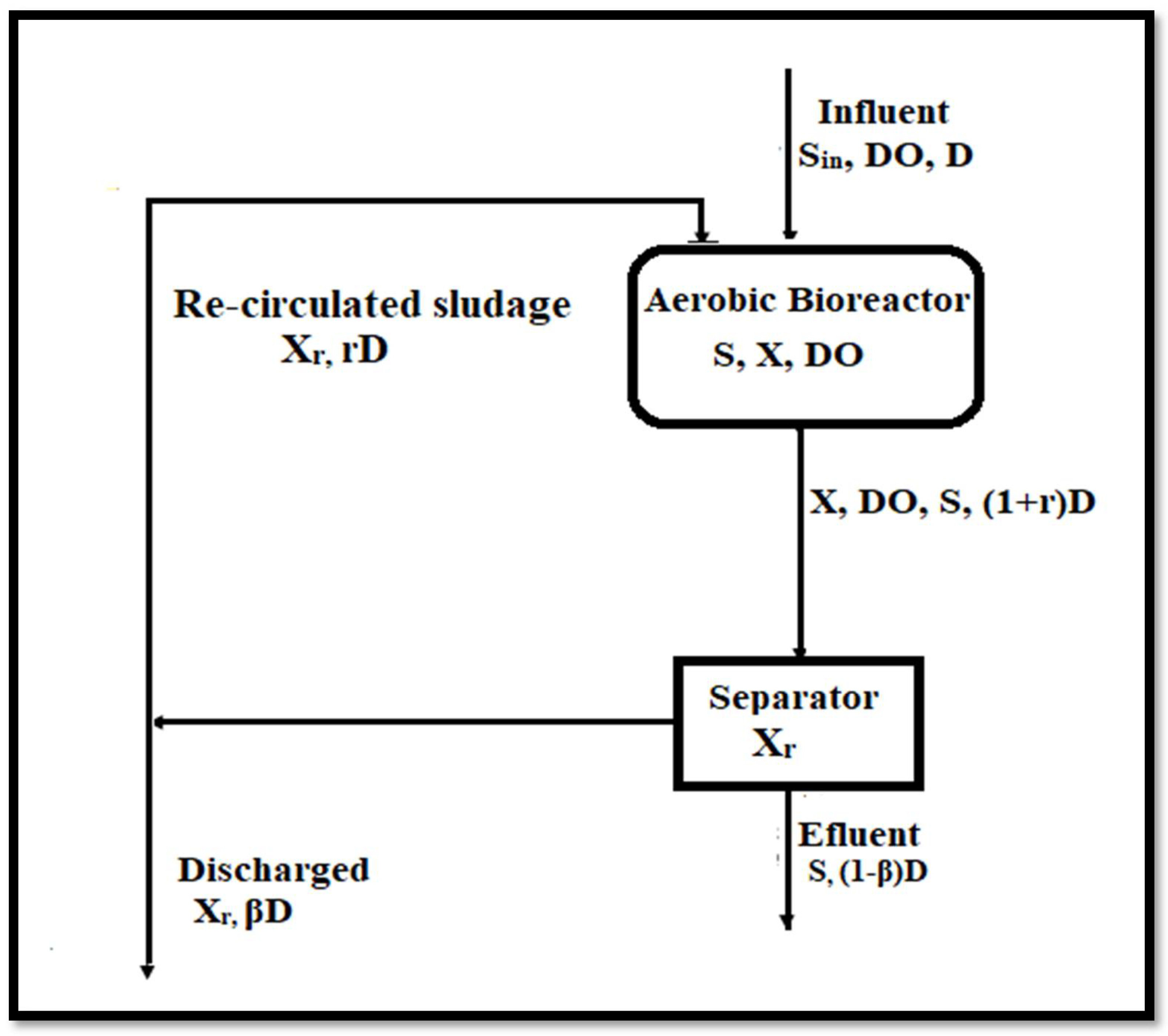
Model equations were used to calculate the concentrations of microorganisms, biodegradable particles, inert material, and soluble substrate in a well-stirred, well-aerated bioreactor. The assumption that the membrane bioreactor is well-agitated means that the substrate is combined with the membrane bioreactor contents instantly and uniformly. Because the reactor is well-aerated, oxygen is not a rate-limiting material. We further assume that the flow through the membrane bioreactor is rapid enough that cell growth does not occur on the reactor walls, i.e., there is no biofilm on the reactor walls, and operational variables such as pH and temperature are automatically maintained. For membrane filtration safety, the ideal value (a maximum desired value) of volatile suspended particles is [77]:

$$\mathrm{VSS}=\mathrm{12,000}{ \mathrm{mg} \mathrm{L}}^{-1}$$

(37)

The rate of change of soluble substrate is described by the equation as follows:

$$V\frac{dS}{dt}=F\left(S_0-S\right)+V{\alpha }_h{k}_h{X}_s+V{f}_s{\alpha }_s{k}_d{X}_b-\frac{V{X}_b\mu \left(S\right)}{{\alpha }_g}$$

(38)

The change rate of the biomass:

$$V\frac{d{X}_b}{dt}=F\left(X_{b,0}-X_b\right)+RF\left(C-1\right)X_b+V{X}_b\mu \left(S\right)-V{k}_d{X}_b$$

(39)

The non-biodegradable particles:

$$V\frac{d{X}_i}{dt}=F\left(X_{i,0}-X_i\right)+RF\left(C-1\right)X_i+V{X}_b\mu \left(S\right)-V{f}_i{k}_d{X}_i$$

(40)

The change rate of the biodegradable particles:

$$V\frac{d{X}_s}{dt}=F\left(X_{s,0}-X_s\right)+RF\left(C-1\right)X_s+V{X}_b\mu \left(S\right)-V{k}_h{X}_s$$

(41)

The residence time is calculated by:

$$Ꞁ=\frac{V}{F}$$

(42)

The chemical demand oxygen (COD) is given by:

$$\mathrm{COD}=S+{\alpha }_h{X}_s$$

(43)

The total volatile suspended solids are calculated by:

$$X_t=X_b+X_i+X_s$$

(44)

where the substrate concentration in the membrane bioreactor is S, the bioreactor flow rate is F (dm³ hr ⁻¹), the Monod constant is Ks, and the recycling ratio is R based on volumetric flow rates. The bioreactor volume (dm3) is V, the substrate concentration entering the membrane bioreactor is S0, the biomass concentration is Xb, and the concentration of non-biodegradable particulate material is Xi. The biodegradable particulate substrate concentration is Xs, the feed concentration into the membrane bioreactor is Xj;0 (j = b; I s), and the total volatile suspended solids concentration is Xt. The death coefficient (hr⁻¹) is kd, the fraction of dead biomass converted to the soluble substrate is fs, the fraction of dead biomass converted to inert material is fi, and the hydrolysis rate of insoluble organic compounds (hr⁻¹) is kh. The yield factor for insoluble organic compound hydrolysis is α_h, the yield factor for biomass growth is α_g, and the yield factor for dead biomass conversion to the soluble substrate is α_s. The maximum specific growth rate (hr⁻¹) is μm, and the specific growth rate model (hr⁻¹) is μs.

It is worth noting that we assumed the settling unit is equally effective at concentrating the biological component (Xb) and the particles (Xs and Xi). The units of soluble substrate concentration are indicated by S, while the units of biomass, non-biodegradable particulate material, and biodegradable particulate substrate concentration are represented by X in the following [78]. The recycling concentration factor (C) is used in these calculations, and the settling unit design conditions determine the value of this factor. However, the typical parameter unit for the model are stated in

Table 2. Typical parameter unit for the monod model.

	Parameter	Unit
1	Ks	mg COD L−1
2	S0	mg COD L−1
3	Xi.0	mg VSS L−1
4	Xs.0	mg VSS L−1
5	fs	g VSS
6	Kd	day−1
7	Kh	day−1
8	αg	mg VSS (mg COD)−1
9	αh	mg COD (mg VSS)−1
10	αs	mg COD (mg VSS)−1
11	μm	day−1

below:

Several accurately structured descriptive models for the sludge processes like ASM-1, ASM-2, and ASM-3 were approved [79,80]. The ASM-1 model consists of 13 different equations and eight processes, including the production and decline of heterotrophic and automotive biomass, organic ammonification, and hydrolysis. Aerobic processes, including nitrogen, chemical oxygen, nitrification, and denitrification, may be anticipated in the model. Following biological nutrient removal in an activated sludge system, Henze et al. [81] created the ASM-1 model, which leads to ASM-2 modeling. The biological use of phosphorus was incorporated into the fundamental ASM1 Framework. The biological removal shall be carried out by adding a factor to the model of improved biological deletion of phosphorus as well as by precipitating the chemical deletion of phosphorus. The biological absorption and removal of phosphorus by the activated sludge system exceed the amount removed by a conventional aerobic activated sludge system. The innovative technique of storing organic substrates was further expanded by Henze et al. [82] which improves the modeling of endogenous respiration lysis (decay) by storing organic substrates. The direct integrations of these numerical equations are used to examine the models [83]. Without recycling, Nelson and Sidhu [84] examined the steady states of the model ASM-1 to assess how the reactor’s performance changes in the context of control factors, including oxygen transfer and residence duration. In addition, in residence duration, there is a key bifurcation point that influences reactor performance. During the organic breakdown of carbon dioxide and methane, Mosey [85] investigated four kinds of bacteria. These groupings are methane bacteria that are acid, acetogénic, acetoclastic, and hydrogen-used. A mathematical model was constructed to represent each of the phases of the kinetic processes utilized for simulating the reaction by the Monod model. Kalyuzhnyi [86] created a batch mathematical model of anaerobic glucose digestion, involving five distinct bacterial types: acidic, ethanologenic, acetogenic, and acetic butyrate-degrade, methanogenic, acetoclastic, and hydrogenotrophic. This model also included numerous variables and possible bacterial inhibitors. An earlier kinetic model was created for use in the simulation of the different processes involved in the degradation of the substrate material in an anaerobic batch reactor (ASBR) [87]. Münch et al. [88] constructed and verified the model of volatile acid generation with the literature’s experimental data. In the wastewater process in which sulphates occur in high quantities. Moreover, Knobel and Lewis [89] have created a mathematical model for assessing the process of anaerobic digestion. Their model was based on the Debye-Huckle theory and may be used to determine activity coefficients, including sulphate reduction, hydrolysis, acidgenesis, long chain fatty acid beta oxidation, acetogenesis, and methanogenesis in many other factors. Furthermore, the treatment process is fixed, and corresponding adjustments cannot be made according to changes in time or space [90].

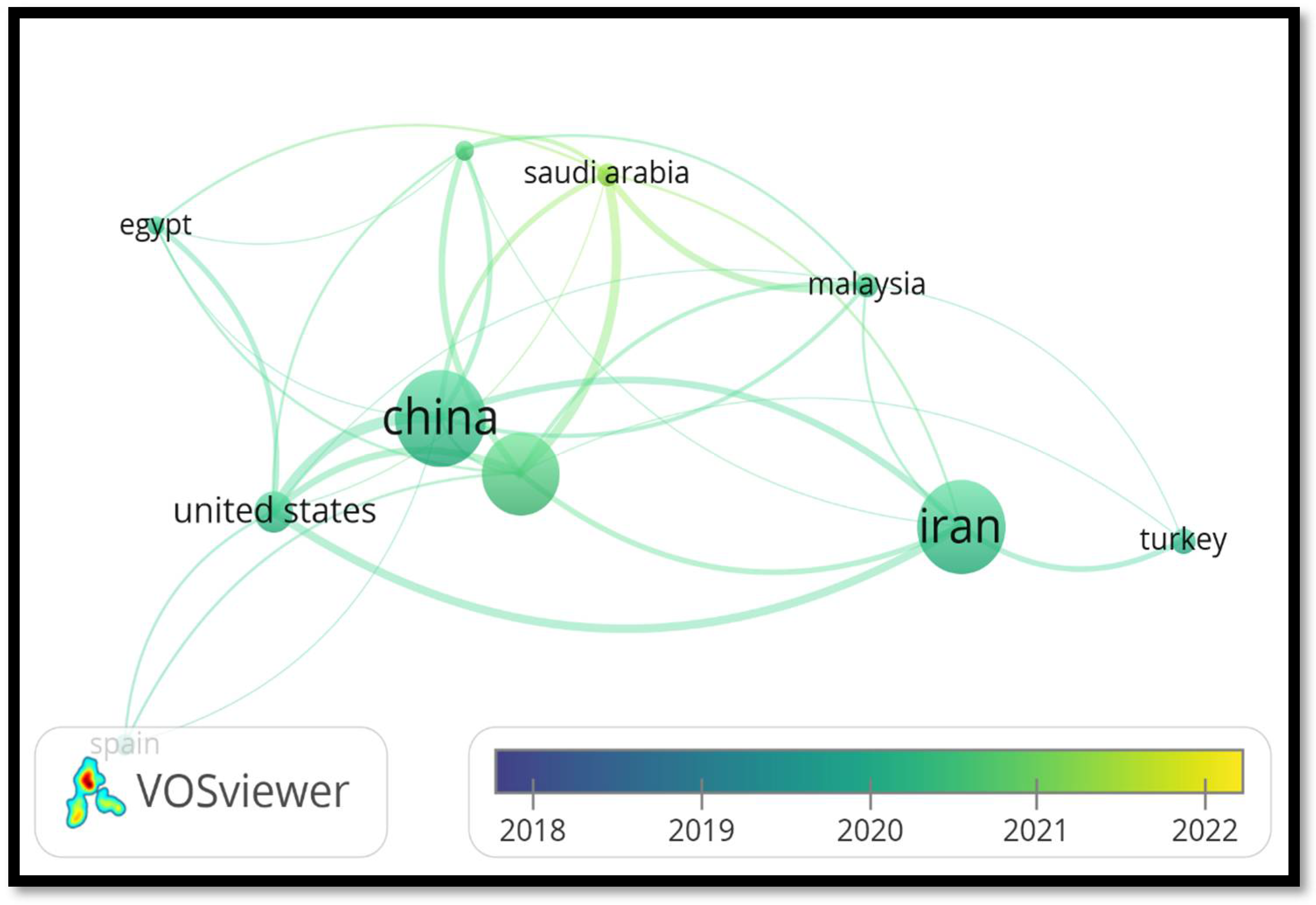
In addition,

Table 3. Top 10 countries according to the number of articles published from 2018 to 2022 in the SCOPUS database for “Monod model and growth rate” keywords.

Country	Documents	Citations	Total Link Strength
India	32	159	2
United States	24	234	5
China	17	204	2
Malaysia	15	58	4
France	12	56	3
Germany	10	103	1
Indonesia	9	20	0
United Kingdom	7	22	1
Canada	6	15	2
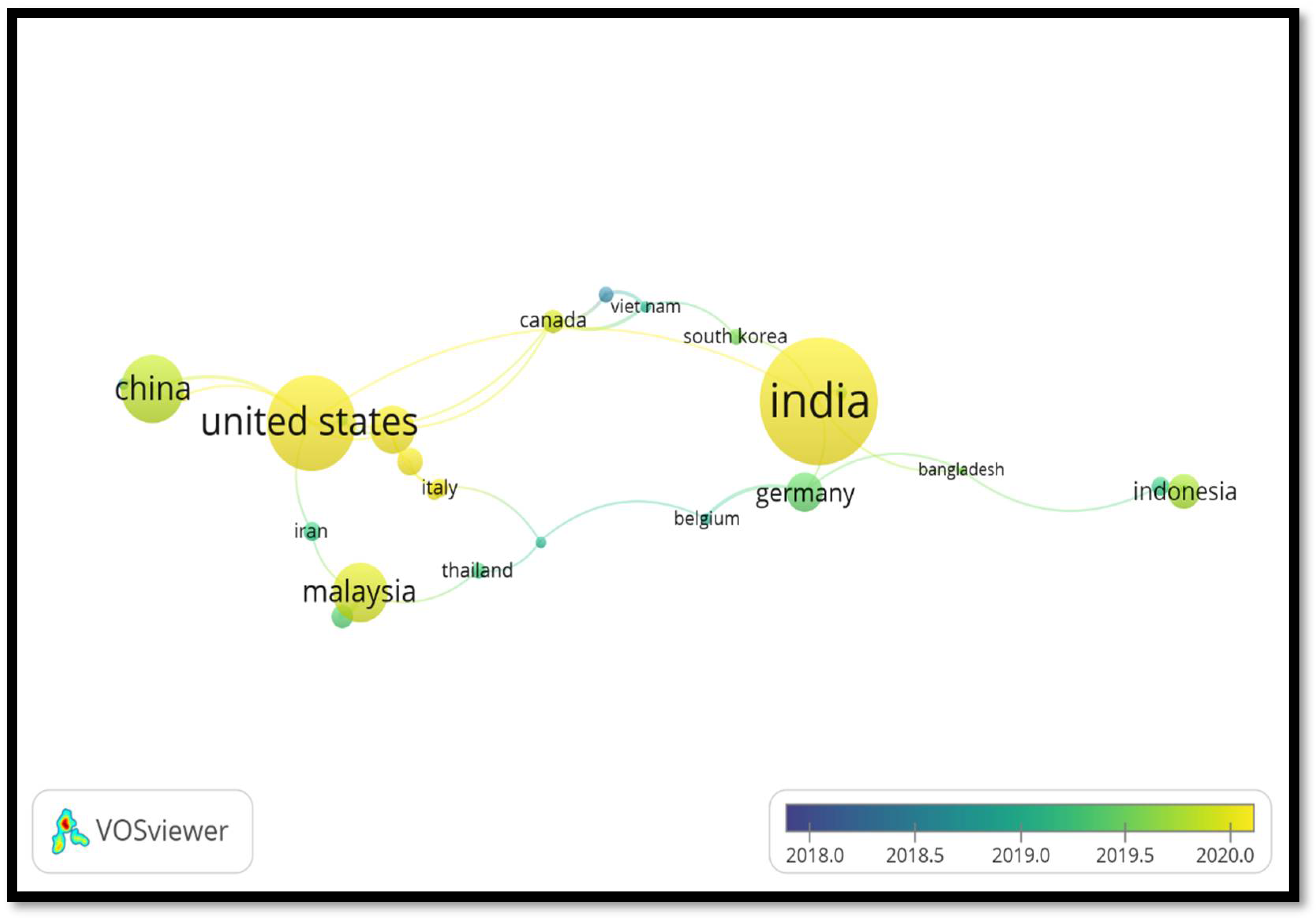
Nigeria	6	23	4

lists the top ten nations based on the number of publications published in the SCOPUS database between 2018 and 2022 that include the keywords “Monod model and growth rate.” Figure 6 also shows the Visualization Network map of the top countries with the most articles published in the SCOPUS database from 2018 to 2022 for the keywords “Monod model and growth rate.”

4.2. Application of the Contois Model

Both aerobic and anaerobic industrial wastewater treatment systems have benefited from the use of the Contois growth model in recent years. The Contois model has been proven to be applicable to the fitting of experimental data for a wide variety of organic materials [91,92,93].

Black olive wastewater was subjected to an aerobic biological degrading process and bio-logical ozonation in the research described by -Beltran-Heredia et al. [94]. The Contois kinetic was utilized to describe the decomposition rate in aerobic biological therapy. It was determined that the Contois model provides an excellent fit to the experimental data, proving that it is applicable to the current experimental setup. Anaerobic treatment of cow dung digesters was explored by Krzystek et al. [95], who looked at the fit of Monod and Contois kinetics to experimental data. According to the comparison’s findings, the Contois kinetic model is superior to the Monod kinetic model for fitting experimental data from cow dung digesters. Using the Monod and Contois kinetic models, Hu et al. [96] studied the process kinetics of the anaerobic digestion of ice cream effluent. The root means square for the Contois kinetic was discovered to be much larger than that of the Monod kinetic. Therefore, the Contois model is more appropriate than the Monod model for modeling the process kinetics of the anaerobic digestion of ice-cream wastewater, i.e., predicting the performance of the anaerobic digester reactor, as indicated by the highest correlation coefficient of 0.918 between experimental data and predicted values obtained from the two models. The Contois model outperformed the Monod model in predicting both microbial growth and the efficiency of the anaerobic digester reactor. The Contois kinetic model accounted for the influence of the influent substrate, hence its forecast was more accurate. Anaerobic digestion of sulfate-rich wastewater was also investigated by Hu, Thayanithy, and Forster [83] using models based on Monod and Contois kinetics in a constantly stirred tank reactor. According to the kinetic investigations, the Contois model was superior to the Monod model in predicting the kinetic reactions of the process, with a correlation value of 0.989. This showed excellent agreement with the experimental data. The Contois kinetic model outperformed the Monod kinetic model in predicting the efficiency of the anaerobic digester reactor and the development of the microorganisms. Therefore, the attachment of biomass to the walls of the reactor, which may supply a source of inoculum, is the reason for the successful prediction of Contois’s kinetic model. Işik and Sponza [97] employed different models, including Monod, Contois, Grau second order, modified Stover-Kincannon, and first-order kinetic, to examine the process kinetics of the anaerobic treatment of textile wastewater in a lab-scale upflow anaerobic sludge blanket reactor. Compared to the Monod and first-order kinetic models, the Contois kinetic model better describes microbial dynamics, as shown by their investigations (r = 0.967). The findings further indicated that the Contois model is the most appropriate one for forecasting anaerobic digester performance. Using the Monod, Chen & Hashimoto, and Contois models, Moosa et al. [98] studied the kinetics of anaerobic sulfate reduction in continuous bioreactors. When it came to defining the dependence of the specific growth rate of bacteria on sulfate concentration, the Contois kinetic model offered the best agreement with experimental results on the anaerobic reduction of sulfate. The removal of sulfate from industrial wastewater and acid mine drainage are only two of the many uses for this technique. Different influent sulfate concentrations were used to calculate the Contois model’s kinetic coefficients. The coefficient for the mortality rate was shown to be stable throughout a wide range of starting sulfate concentrations. Nonetheless, the saturation constant (Ks) rose dramatically with increasing initial sulfate concentration whereas the maximal specific growth rate (max) changed little. Tessier, Monod, and Contois models of biodegradation kinetics were employed to model the process. The experimental data were well-fit by each of the models. However, the strongest correlation value (0.984) was reported for the Contois kinetic model in describing the microbial growth of Xhhh growth. Abdurahman et al. [99] also studied the treatment of palm oil mill effluent utilizing a membrane anaerobic system, but they did it via the lens of three kinetic models: the Monod, Contois, and Chen & Hashimoto models. Both investigations demonstrated that the Contois model had a very good fit for experimental data (r = 0.962 and r = 0.997, respectively). The greatest value for the correlation coefficient was obtained using the Contois model in the second scenario. Methane generation rate from anaerobic digestion of cow dung in bench-scale gas-lift digesters was predicted using a novel model presented by Karim et al. [100] proposed a new model, including the Contois kinetic model and an endogenous decay model to predict the methane production rate from the anaerobic digestion of cow manure in bench-scale gas-lift digesters. The proposed model and two other well-known kinetic models, the Hill [101] models, which included the Contois kinetic model and an endogenous decay model. The experimental data for methane production rate was fitted using the suggested model and two additional well-known kinetic models, the Hill [95] models. Although the Chen and Hash-imoto and Hill models performed poorly in fitting the experimental data (correlation coefficients of 0.86 and 0.51, respectively), the novel model including Contois kinetics performed very well (r = 0.99). The suggested model, which incorporates the Con-tois model, performed better than the other two models in predicting the rate of methane generation when compared to experimental data. For the hydrolysis of particulate organic material in anaerobic digestion, Vavilin et al. [102] examined four kinetic models, including Monod, first-order, two-phase, and Contois kinetics. The acquired findings demonstrated that good fits to the experimental data could be achieved by using the Contois kinetic for the hydrolysis kinetics of swine waste, sewage sludge, cow manure, and cellulose. The lactate fermentation properties of B. Coagulans in a batch reactor were modeled by Hidaka et al. [103] Substrate, lactate (product), sodium chloride, and bacterial growth were all accounted for in the model as inhibitors. The degradation of carbohydrate particles was simulated using the Contois kinetic model. Based on their findings, they concluded that the Contois model is superior to the first-order reaction model for modeling the hydrolysis of kitchen trash particles. Anaerobic hydrolysis of organic waste particles is described using the Contois model, and this finding is consistent with previous work [34,104] that employed this model.

In many analyses, researchers found that the Contois equation well described the kinetics of fungal growth. The growth kinetics of the fungus Rhizopus nigricans in response to glucose was investigated by Zhou et al. [105] using the Contois model. With a correlation coefficient of 0.99, the findings demonstrated the validity of the Contois model for modeling the kinetics of cell growth.

The Rhodotorula red yeast strains that Hernalsteens and Maugeri [106] studied generated an extracellular enzyme. The Contois model was used to characterize the microbial growth dynamics. In contrast to the standard Monod model, the Contois model was shown to provide an excellent match to the experimental data (r = 0.95).

Furthermore,

Table 4. Top 10 countries according to the number of articles published from 2018 to 2022 in the SCOPUS database for “Contois model and growth rate” Keywords.

Country	Documents	Citations	Total Link Strength
France	7	26	2
India	7	41	0
Australia	5	89	3
Iran	5	83	2
China	5	92	1
Indonesia	5	13	0
United States	4	60	2
Canada	3	17	2
Saudi Arabia	3	24	2
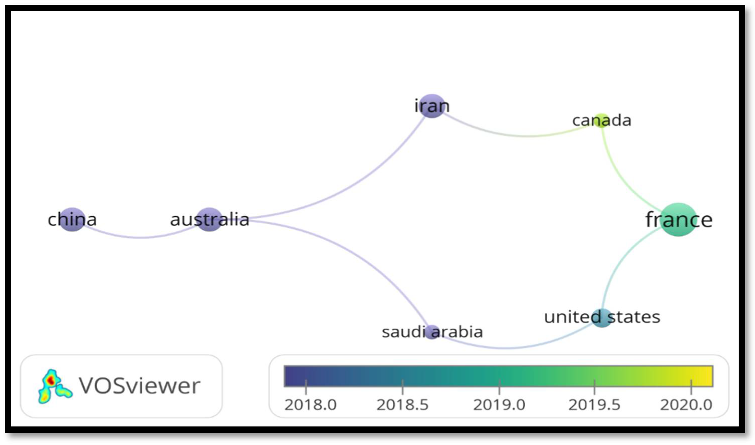
Malaysia	3	9	0

displays the top ten countries based on the number of articles published in the SCOPUS database between 2018 and 2022 with the keywords “Contois model and growth rate.” Figure 7 also illustrates the Visualization Network map of top countries published in the SCOPUS database, as well as the relationship between them, from 2018 to 2022 for the keywords “Contois model and growth rate”.

4.3. Application of RSM

Relational statistical modeling (RSM) uses experimental data to construct mathematical models that characterize the associations between causes (independent variables) and response variables (responses). Independent variables and interaction effects on responses are analyzed and optimized using these models. 2-D contours and 3-D plots are the most common ways to display the findings. To implement the RSM, one must use statistical experimental design, linear regression modeling, and optimization techniques. The process of using RSM as an optimization technique consists of many phases. The steps are (i) deciding on which variables to use and what ranges to use them in, (ii) deciding on an experimental design and carrying it out, (iii) generating a linear regression model equation from the experimental results, (iv) checking the model’s sufficiency, and (v) visualizing the model to determine the best settings.

Multiple process factors affect the efficacy of the various procedures used in water and wastewater treatment. If these procedures could be optimized to provide optimum results, not only would costs be reduced, but so would the usage of precious resources like energy and materials. The conventional way of optimizing a problem involves considering just a single variable at a time. With this method, we may isolate the effects of a single variable by holding all others constant. This process is then repeated with more variables until the optimal circumstances are achieved. However, this method cannot provide a full picture of the impacts of the variables on the process since it does not show the interaction effects among the variables evaluated. The one-factor-at-a-time method is both time-consuming and expensive since it requires several experiments [107].

The design of experiments has been used to find solutions to these issues. The design of experiments has several benefits, such as the ability to learn the same amount with fewer trials, estimate relationships between components, and create empirical models. The response surface methodology (RSM) [108] is a technique for designing experiments from a graphical viewpoint. Response Surface Methodology (RSM) is a set of mathematical and statistical methodologies for getting the optimal conditions for responses with a minimal number of scheduled tests [109].

Recent years have seen an increase in the use of RSM for optimizing and analyzing various water and wastewater treatment processes, including coagulation-flocculation, adsorption, advanced oxidation processes, electrochemical processes, and disinfection. The availability of various RSM-specific computer programs has made implementing RSM a very straightforward undertaking. However, it has also led to the inappropriate application of RSM. For the RSM to be successfully used, both the process being researched, and its limits and applicability must be understood in depth.

Heavy metals and harmful organic compounds may be removed from water by the use of adsorption and biosorption methods, which are utilized in water and wastewater treatment. In adsorption, the ions or molecules in a solution are focused on an appropriate contact. pH, ionic strength, adsorbing surface type, and adsorbent/adsorbate ratio all play significant roles in the adsorption process [110]. The present article provides a review of some of the published research that uses RSM to optimize operational parameters during adsorption and biosorption.

The removal of methyl orange dye by activated carbon was studied by Tripathi et al. [111] using the RSM with Box–Behnken Design. Adsorbent dosage (5–20 mg/L), contact period (2-6 h), temperature (25–55 W C), and pH were all taken into account (2–8). The optimum conditions of adsorbent dosage = 15.7 mg/L, contact duration = 4 h, temperature = 40 W C, and pH = 2 resulted in a 99.11% removal efficiency. Using the noxious plant Parthenium hysterophorus as a cheap adsorbent, Chatterjee et al. [112] investigated methylene blue removal. By using RSM, we were able to statistically optimize the factors involved in both adsorbent preparation and dye removal and recovery. Carbonizing parameters studied included activating agent to Par-thenium weight ratio (1.0–1.5), carbonizing temperature (450–550 W C), and carbonizing duration (1–2 h). Response decolorizing power was maximized at a weight ratio of 1.05:1 and after being carbonized at 550 °W for 1 h. The cleaned sample was put to use in further research on dye elimination. Initial dye concentration (25–50 mg/L), adsorbent weight (0.2–0.5 mg/L), pH (5–8), and temperature (25 C–35 C) were all taken into account (30–40 WC). The optimal conditions for maximal dye removal were 25 mg/L starting concentration, 0.5 g adsorbent weight, pH 7, and 35 °C. The independent factors used to determine the most effective dye recovery method were the quantity of wasted adsorbent (0.2–0.5 g), pH (5–9), and contact duration (1–3 h). The model showed that the recovery rate increased both with decreasing pH and with increasing contact duration. Biosorption of heavy metals including Cu(II), Ni(II), and Zn(II) on surfactant-modified chitosan bead was optimized using RSM by Sarkar and Majumdar [113]. For this reason, a half factorial design with 251 components was used to determine which ones were most relevant. After a series of trials, the optimal values for pH, metal concentration, and adsorbent dose were determined. For the same amount of adsorbent, more adsorption occurred when more adsorbent was used. Through RSM with a central composite design, the optimal parameters for Cu(II) adsorption were determined to be pH 5.5, adsorbent dose 0.5 g/L, and starting concentration of 30 mg/L.

The increased oxidation of direct red 28 dye by photo-Fenton treatment with RSM was studied by Ay et al. [114]. The experimental layout was a Box–Behnken design. Color and total organic carbon (TOC) removals were studied to determine the impact of dyestuff concentration, peroxide dosage, and Fe(II) dose. It was shown using RSM modeling that the efficiency of color removal decreased as a function of dyestuff concentration while improving with increasing H₂O₂ and Fe(II) dosages. Dyestuff, H₂O₂, and Fe(II) dosages all contributed to greater TOC elimination. The estimated ideal peroxide/Fe(II) ratio at the highest starting dyestuff concentration of 250 mg/L was 715/71 mg/L for 100% color removal, and this ratio was 1.550/96.5 mg/L for 97.5% TOC removal.

The electro-Fenton procedure employing RSM was studied by Mohajeri et al. [115] to remove stubborn organics from semi-aerobic landfill leachate. The experimental runs were planned using a central composite design, with the molar ratio of H₂O₂ to Fe²⁺, current density, pH, and reaction duration serving as input variables and the elimination of COD and color serving as responses. The experimental design was simplified by holding constant the remaining variables, including temperature, stirring rate, and electrode separation. The optimal parameters found to remove 94.16% COD and 95.83% color were a current density of 40 mA/cm², a pH of 3, a reaction period of 43 min, and a molar ratio of H₂O₂/Fe²⁺ of 1. Values from validation studies were found to be in reasonable agreement with these.

By identifying the optimal operating conditions for a system and creating a response surface model that predicts a response based on a combination of factor levels, RSM is a very effective process. More so, it details how several variables influence the final result and how those aspects interact with one another. Because of this, they have found widespread use in the modeling of water and sewage treatment systems and processes, as this overview demonstrates.

The majority of published research on optimizing systems or processes did so without taking economic factors into account. This means that it is important to consider cost when trying to find the best configuration for a system or process, and fortunately, RSM makes this very easy to do. In addition, RSM may be used to pinpoint an area of the factor space where all the necessary operational conditions hold. When it comes to water and wastewater treatment systems, where many regulations and requirements must be satisfied, this is of paramount importance.

The experimenter’s background knowledge of the process under investigation is essential for generating reliable results from an RSM analysis. Evidence from this research indicates that, in many experiments involving optimization, true optimum points were not located because the range of independent variables was incorrectly chosen, causing the optimal circumstances to lie outside the experimental area. Conditions associated with maximum/minimum responses are incorrectly represented as optimal in such cases. This demonstrates the need of doing the necessary groundwork beforehand to determine the appropriate range of independent variables in experimental design.

There is a wealth of material on the use of RSM in the lab for water and sewage purification, but very little on its actual use in the real world. As a result, additional research into the method’s potential practical uses is required. Additionally, further study is required to evaluate and integrate RSM with other modeling approaches such as ANN and fuzzy logic for modeling various water and wastewater treatment processes.

Additionally,

Table 5. Top 10 countries according to the number of articles published from 2018 to 2022 in the SCOPUS database for “response surface methodology and wastewater treatment” keywords.

Country	Documents	Citations	Total Link Strength
Iran	294	3972	42
China	258	2704	43
India	255	2560	48
Malaysia	144	1159	49
Turkey	81	792	19
Saudi Arabia	70	720	67
Brazil	49	541	20
Pakistan	44	283	43
United States	44	471	36
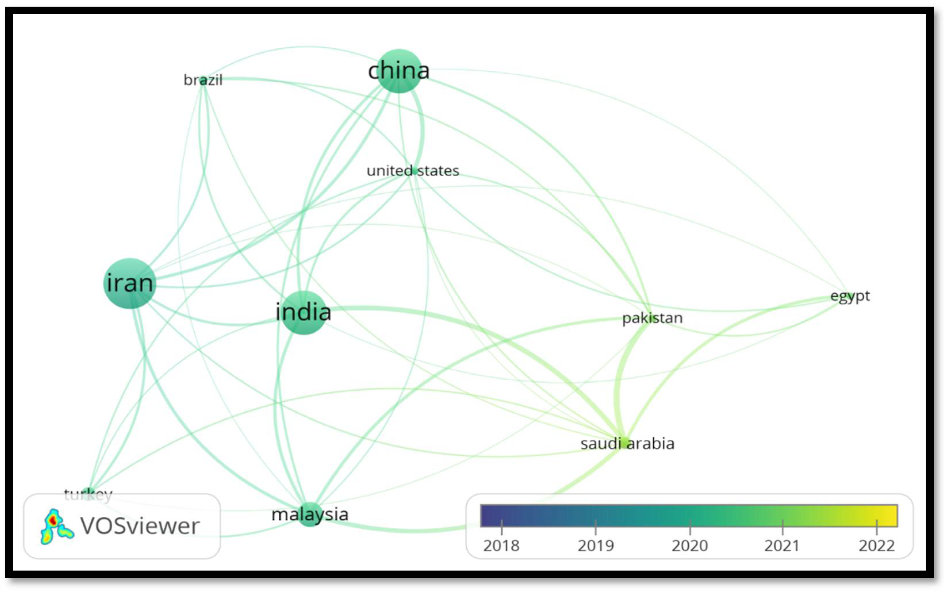
Egypt	41	398

lists the top ten nations based on the volume of publications containing the keywords “response surface methodology and wastewater treatment” that were published in the SCOPUS database between 2018 and 2022. Figure 8 also shows the Visualization Network map of the most popular nations from 2018 to 2022 for the keywords “response surface methodology and wastewater treatment,” along with the relationships between them.

4.4. Application of ANN

Treatment of wastewater is a complex nonlinear system characterized by significant random disturbance, time fluctuation, and uncertainty. Current wastewater treatment plant planning and operations are based mostly on experiments, which leads to significant inaccuracies. In-depth studies have been conducted on the system for years, and several mechanism models have been proposed, but due to complexity and uncertainty, real-time control has not yet been achieved. 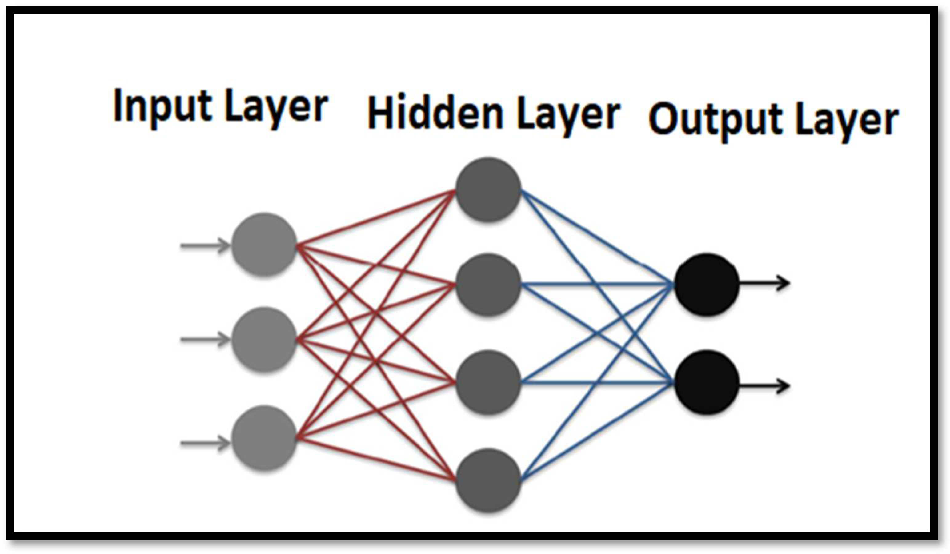Artificial neural networks (ANN) have been the focus of a great deal of study [116,117] due to their capacity to provide approximations to complicated and nonlinear equations. A neural network (ANN) is a kind of information processing system that takes its cues from the study of biological brain processing. Biological neural networks are composed of many individual neurons that are non-linear and densely coupled. To facilitate its logical parallelism, an ANN organizes its neurons into layered structures. In serial operations, information is sent from one layer to another [118]. An ANN’s fundamental structure typically consists of three different levels: an input layer, where data are supplied to the ANN; a hidden layer or layers, where data are processed; and an output layer, where the findings of the ANN are shown. Adjustable rules specify the relative relevance of weights for input. The ANN is constructed by applying weights between neurons and a transfer function that regulates the formation of the output. During training, the ANN assigns relative significance to the weights and fine-tunes them using iterative methods [119].

Using water temperature, SS (suspended solid) concentration, influent COD concentration, NH3-N, MLSS, MLVSS, and SV30 (volume ratio after 30 min settlement), Yang et al. [120] proposed a stable and sensitive dynamic neural network model for predicting effluent quality and potential real-time adjustment of wastewater treatment operations.

As a means of training a well-designed neural network, Liu [121] employed analog data input and output from EFOR software based on activated sludge mathematical models, and then modified the input and compared it to the output. The findings suggested that the neural network might be used for dynamic modeling of biological nitrogen and phosphorus elimination. In order to predict effluent TP and TN from the carrousel oxidation ditch system in a wastewater treatment plant, Chen et al. [122] used an RBF neural network. Principal component analysis and cluster analysis were helpful in data mining during the model-building process, and preprocessing the data was essential in lowering the prediction error rate. With TN 94% accuracy and TP 70% accuracy in effluent parameter predictions, the neural network has an excellent performance in tests and can adapt to different scenarios. According to the results of the correlation coefficient test, TN was 0.95 and TP was 0.89.

Based on the multiple neural networks, Yu et al. [123] suggested an effluent quality prediction model. The input space is partitioned into numerous subspaces using subtractive clustering, and matching models are constructed using a neural network. After that, the models are integrated using principal component regression to get rid of the high degree of correlation between them and boost the model’s precision and stability (PCR). Additionally, a modified objective function and weighted feedback correction are used to enhance the model’s generalization capacity and prediction accuracy of the high measured value. The effluent from a wastewater treatment facility is tested for NH3-N ammonia nitrogen using the suggested approach, and the findings are promising.

Effluent from an SBR may be used to calculate BOD content using a soft sensing approach suggested by Liu et al. [124], which is based on the radial basic function (RBF). The SBR analysis led us to choose TOC, DO SS, and response time as input variables, and TOC as the desired outcome. Then, using the established correlation between TOC and BOD5, BOD5 was acquired by conversion. We trained an RBF neural network and found that its simulation may be utilized to calculate BOD5 for controlling the wastewater treatment process in real-time

To predict BOD5 and COD in treated wastewater drainage, Xu and Pan [125] used a sophisticated model including a support vector machine (SVM) and features between BOD5 and COD. This approach to SVM parameter optimization uses a particle swarm optimization algorithm, which has superior search abilities and was proposed to address the issue of parameter selection in SVM. The parameters of the control system for wastewater treatment are then collected using soft sensing.

For sequential wastewater treatment operations, Wang et al. [126] provided a complete assessment on the soft-sensing of water quality in a wastewater treatment process (WWTP) using artificial neural networks (ANNs). They primarily offered issue formulation for water quality soft-sensing, typical soft-sensing models, practical soft-sensing examples, and a discussion of soft-sensing model performance.

Simultaneous determination of Au and Pd concentration in wastewater was performed using BP neural network-spectrophotometry approach, as described by Zheng et al. [127]. To improve its solubility and sensitivity to test Fe, Ni, and Cu in wastewater, Mingjin [128] created wavelet packets with analysis-simple recurrent neural network (Elman) spectrophotometry using 5-Br-PADAP as a colorizing agent in the presence of nonionic surfactant.

Since the physical phenomena for As (III) and As (VI) removal by individual bacterial Biomass [8] and mixed dried biomass [7] is complex, the prediction of As (III) and As (V) adsorption using an artificial neural network (ANN) model is involved. An ANN model, based on 128 sets of experimental data, was developed to simulate the way the human brain works. The ratio of input neurons to those in the hidden layer to those in the output layer was 5-7-1. Of the batch data, 75% was set aside for the learning process, 10% for the testing phase, and 15% for the validation. There was very little mean squared error and a very high degree of correlation (R2 = 0.9959) between the projected output vector and the experimental data (MSE; 0.3462). The suggested model’s anticipated results matched the batch work within a tolerable margin of error. An ANN model, based on batch experimental data, was developed to simulate the human brain’s processing capabilities. An equal number of neurons (5-7-1) were distributed throughout the input, hidden, and output layers. It was decided that 75% of the batch data would be used for instruction, 10% for experiments, and 15% for verification. Predicted results from the suggested model were found to be in fair agreement with batch experiments. Meanwhile, during testing and training, we looked at the network’s mean squared error (MSE) and mean error to gauge its performance. However, the training phase was crucial in demonstrating the network model’s capacity to anticipate responses to batches of data. For this reason, it is advised to observe both the mean squared error (MSE) and the mean error during the testing and validation processes, since both metrics are uniquely suited to assessing the model’s efficacy. After 188 iterations, the optimal output vector for a specific set of experimental data input was found, with a minimal MSE of 0.6131. Furthermore, it was found that the mean error (M) and mean square error (MSE) for the training data were 0.1091 and 0.6131, respectively, whereas the corresponding values for the testing data were 0.0767 and 0.3462. In terms of statistical indicators (correlation coefficient), values of 0.9909 and 0.9959 were attained for the training data and the testing data, respectively.

Even though there have been several studies on the use of neural networks in wastewater treatment, most of the techniques are still only used in the lab. There is a need for further research into using neural networks for full and high-quality control of wastewater treatment. The integration of neural networks with other control methods is an intriguing area to investigate due to the networks’ superior research capabilities and inherent flaws. The use of ANN is regarded as a successful approach owing to its versatility in simulation, estimation, and modeling. The significance of ANN is that it is structurally consistent and can learn from previous data. Furthermore, the main advantage of ANN over RSM is that it does not require a prior specification of the best fitting function and has universal approximation functionality, i.e., it can approximate nearly all types of nonlinear functions, including quadratic functions, whereas RSM is only useful for quadratic approximations [129,130,131]. Although ANN has gained popularity for its usage in a variety of engineering domains, several studies for modeling and improving adsorption processes have used this technique [132,133].

In addition, the top ten nations are ranked in

Table 6. Top 10 countries according to the number of articles published from 2018 to 2022 in the SCOPUS database for “artificial neural networks and wastewater treatment” Keywords.

Country	Documents	Citations	Total Link Strength
China	100	1203	28
Iran	98	1370	24
India	85	673	31
United States	42	543	29
Turkey	26	278	6
Malaysia	24	283	17
Saudi Arabia	23	189	24
Spain	22	247	5
South Korea	20	265	18
Egypt	19	254	10

according to the total number of articles containing the keywords “artificial neural networks and wastewater treatment” that are expected to be added to the SCOPUS database between the years 2018 and 2022. Figure 9 also provides an illustration of the Visualization Network map of the top nations published in the SCOPUS database from 2018 to 2022 for the keywords “artificial neural networks and wastewater treatment”, as well as the link between these countries.

5. Conclusions

The Monod, Contois, response surface methodology (RSM), and artificial neural networks (ANN) models were used in this research to explore wastewater treatment processes. Despite this, the study also revealed mathematical modeling for biological wastewater treatment. The Monod and Contois model will be used common assumptions, in bioprocess engineering, to imitate the specific growth rate. Furthermore, the artificial neural networks (ANN) and response surface methodology (RSM) models are used for wastewater treatment. This review suggested that the specific microorganism growth rates were determined by the Contois growth model and optimizing and predicting the wastewater treatment process were obtained with high accuracy by artificial neural networks (ANN). As a consequence, the Contois and ANN models capture the individual growth rate and biological wastewater treatment better than other models. Further experimental tests are required in the future to prove the accuracy of this model for predicting microbial growth and wastewater treatment processes.