Comparison of CLDAS and Machine Learning Models for Reference Evapotranspiration Estimation under Limited Meteorological Data

Abstract

The accurate calculation of reference evapotranspiration (ET₀) is the fundamental basis for the sustainable use of water resources and drought assessment. In this study, we evaluate the performance of the second-generation China Meteorological Administration Land Data Assimilation System (CLDAS) and two simplified machine learning models to estimate ET₀ when meteorological data are insufficient in China. The results show that, when a weather station lacks global solar radiation (R_s) data, the machine learning methods obtain better results in their estimation of ET₀. However, when the meteorological station lacks relative humidity (RH) and 2 m wind speed (U₂) data, using RH_CLD and U_2CLD from the CLDAS to estimate ET₀ and to replace the meteorological station data obtains better results. When all the data from the meteorological station are missing, estimating ET₀ using the CLDAS data still produces relevant results. In addition, the PM–CLDAS method (a calculation method based on the Penman–Monteith formula and using the CLDAS data) exhibits a relatively stable performance under different combinations of meteorological inputs, except in the southern humid tropical zone and the Qinghai–Tibet Plateau zone.

1. Introduction

Reference evapotranspiration (ET₀) is an important consideration when estimating crop evapotranspiration [1] and comprises essential data for planning and designing farmland water conservancy projects [2]. It plays a vital role in accurately estimating water resource management, regional water balance, drought assessment and climate change [3]. Currently, the Penman–Monteith (FAO-56 PM) method recommended by the Food and Agriculture Organization of the United Nations (FAO) is the standard calculation method for ET₀. This approach, which integrates energy balance with aerodynamic theory, is highly applicable to various geographic and climatic contexts [4], but requires air temperature (T), relative humidity (RH), solar radiation (R_s) and wind speed (U) data, as well as other meteorological factors. However, the distribution of meteorological stations in China is uneven, making it difficult to obtain accurate and complete meteorological data in many regions. Therefore, using limited meteorological data to obtain high-precision ET₀ has attracted much attention.

Due to the growth of machine learning algorithms in recent decades, many researchers have used meteorological data to estimate ET₀ based on machine learning and have developed models with great accuracy. In addition, machine learning is popular because of its ability to handle massive datasets and compute results quickly. As increasing amounts of data are provided to the system, machine learning models can produce more accurate results over time through self-learning, without requiring new codes and algorithms. At present, there are three main types of machine learning algorithm with high fitting accuracy: (1) kernel function algorithms, such as support vector machine (SVM) and the kernel-based arps decline model (KNEA); (2) tree integration algorithms, such as random forest (RF), categorical boosting (CatBoost) and extreme gradient boosting (XGBoost); and (3) neural network algorithms, such as generalized regression neural networks (GRNNs) and extreme learning machine (ELM). In relation to the semi-arid regions in Iran, Tabari et al. (2012) [5] used a SVM and an adaptive neuro-fuzzy inference system (ANFIS) to estimate ET₀, and the prediction results were superior to those of the empirical models. Wu and Fan (2019) [6] applied the KNEA and SVM to predict daily ET₀ in different regions of China, and the results showed that both SVM and KNEA had sound prediction effects. Feng et al. (2017) [7] conducted an ET₀ forecast study of humid regions in southwestern China, showing that random forest (RF), based on temperature and radiation data, had a good forecasting effect. The potential of a new machine learning approach by which to employ gradient boosting on decision trees with categorical feature support was examined by Huang et al. (2019) [8], and the results demonstrated that, in humid regions of China, the CatBoost algorithm had an extremely significant potential for ET₀ estimation. Liu et al. (2021) [9] studied how to improve the adaptability and accuracy of machine learning to simulate ET₀ in Jiangxi Province, and found that Gaussian process regression (GPR) and limit gradient boosting (CatBoost) models had higher prediction accuracy. Wang et al. (2017) [10] and Zhang et al. (2018) [11] used 15 different combinations of meteorological factors, such as maximum temperature (T_max), minimum temperature (T_min), wind speed and relative humidity, and the RF and ELM machine learning methods. They compared these with the traditional temperature-based Hargreaves method to predict ET₀, and it was found that the accuracy of the RF and ELM models was better than that of the Hargreaves method in different situations. Feng et al. (2017) [12] conducted ET₀ modeling at six meteorological stations in the Sichuan Basin, China. Their findings revealed that both temperature-based GRNN and ELM performed better than the Hargreaves method. Thongkao et al. (2022) [13] selected five calculation models, including random forest (RF) and M5 model tree (M5), to estimate the b factor in the calculation process. The research results showed that the support vector regression with the radial basis function kernel (SVR-rbf) performed best among the five models, followed by M5, RF, support vector regression with the polynomial function (SVR-poly), and random tree (RT).

In addition, the data from meteorological stations in some areas are not comprehensive, and these missing meteorological data will affect the estimation of ET₀. However, in recent years, many scholars have begun to use limited meteorological element data to calculate ET₀ based on machine learning methods and have achieved high accuracy. Ferreira et al. (2019) [14] used a SVM and an ANN to estimate ET₀ in Brazil under limited meteorological data, and the results indicated that both techniques produced acceptable prediction outcomes. Bakhtiari et al. (2016) [15] evaluated the ability of three machine learning models, including support vector machine (SVM), to calculate ET₀ in the case of limited meteorological data in order to study the reference evapotranspiration in semi-arid areas of Iran. The findings indicated that the machine learning approach performed better than the empirical model. Chia et al. (2017) [16] used an ANFIS method to estimate the ET₀ in eastern Malaysia with limited meteorological data, and the results demonstrated that the ANFIS model was capable of providing precise forecasts.

Reanalysis datasets have also been developed simultaneously and have been frequently utilized in water-resource management research and other fields in recent years [17]. The most cutting-edge massive data assimilation systems and excellent databases are used with reanalysis data. This comprises a full range of reanalysis data that have been acquired through quality assurance and assimilation of observation data from multiple sources (ground, ship, radio sounding, wind balloon, aircraft, and satellite). The data not only contain various elements and have a large range, but also have a long extension period and a high resolution. Datasets from global atmospheric reanalysis can offer the necessary inputs for estimating ET₀ [18].

The application of reanalysis data in water-resource management research has the following two advantages [19]: (i) data continuity over a long period of time, whether at a global or local level, and (ii) open availability of data to the public for free via specialized web platforms that prepare these data for use in common formats, reducing the time-consuming processes needed to acquire and homogenize weather station data from various service providers. The spatial distribution of meteorological stations in China is not uniform, making it difficult in some rural areas to collect observation data in respect of various climate variables. This data scarcity is supplemented by reanalysis datasets, which are highly accurate and have a high spatial resolution. They are widely used in hydrological modeling and have been effectively employed by numerous authors to indicate surface climate variables’ spatiotemporal variability [20,21,22].

Reanalysis data have been used to predict and compare evapotranspiration in different regions. Based on climate forecast reanalysis data, Woldesenbet et al. (2021) [23] calculated the ET₀ in the Omo-Gibetta watershed and obtained promising forecasting results. Srivastava et al. (2015) [24] found that the medium-term ERA predicted ET₀ more accurately than the estimation of ET₀ of the National Center for Environmental Prediction/National Center for Atmospheric Research (NCEP/NCAR). Pelosi et al. (2020) [25] also contrasted two reanalysis datasets for ET₀ estimation in southern Italy. Tian and Martinez (2012) [26] calculated ET₀ in south-eastern United States using the NCEP reanalysis dataset. Song et al. (2015) [27] evaluated the spatiotemporal properties of reference evapotranspiration in Shaanxi Province using the NCEP reanalysis data and generated projections for the future. The Poyang Lake basin’s ET₀ was estimated by Liu et al. (2019) [28] using the CMIP5 model. The results show that the ET₀ calculated from the NCEP reanalysis data has a good correlation, and the accuracy is significantly improved after deviation correction, making it suitable for estimating future ET₀ of Poyang Lake basin. Martins et al. (2016) [29] evaluated ET₀ inside the Iberian Peninsula; the goal was to apply an NCEP/NCAR hybrid reanalysis product and a gridded dataset to estimate ET₀, and the results show that the reference evapotranspiration estimated using the mixed reanalysis has a high correlation with the measured data at the station (root mean square error, RMSE = 0.49 mm/day). Raziei (2021) [30] estimated monthly ET₀ for 43 weather stations spread over Iran through using NCEP/NCAR reanalysis together with a gridded dataset, and the results demonstrate that the mixed reanalysis calculation of ET₀ has a greater effect than the majority of ET₀ calculations based on research station observations. Milad and Mehdi (2022) [31] used the reanalysis product ERA5 to obtain more accurate results for daily and monthly ET₀ estimates under limited data. With the continuous advancement of numerical weather models and computational and data assimilation techniques, the accuracy of satellite-derived atmospheric and ground data, and the geographical and temporal resolution and dependability of reanalysis data have all steadily improved over time. However, unlike this study, the above studies generally refer to a small catchment area and a short time-step computational approach.

The more mature land surface data assimilation systems available today include the US Global Land Data Assimilation System (GLDAS), the North American Land Data Assimilation System (NLDAS) and the Korean Land Data Assimilation System (KLDAS) [32]. In 2017, the China Meteorological Administration (CMA) completed its second-generation Land Data Assimilation System (CLDAS), covering East Asia [33,34]. In China, CLDAS is the sole real-time service system for assimilation of land surface data. To merge data from diverse sources, including ground observation, satellite observation, and numerical model outputs, it combines fusion and assimilation technologies [28]. The system’s output comprises high temporal and spatial resolution land-surface driving products, such as temperature, air pressure, specific humidity, wind speed, precipitation, solar shortwave radiation and soil moisture, which could be utilized in the monitoring of agricultural drought, the assessment of climate system models, mountain and flood geological disaster meteorological services, and the provision of fine spatial grid accurate data. Some of these elements, such as surface soil moisture [35], surface soil temperature [36] and near-surface air temperature [37], have been assessed but have not yet been used to calculate ET₀ for major land areas in China and to conduct a comprehensive and detailed assessment. The evaluation of ET₀ is a crucial component of the study of climate change, serving as a useful guide and having practical value for comprehending regional ecological changes and advancing sustainable development [38].

In conclusion, there is confusion regarding whether to use reanalysis data or machine learning to calculate ET₀ when meteorological data are insufficient. Therefore, in this study, we aimed to evaluate whether the CLDAS data or a machine learning simplified model is more suitable for estimating ET₀ when meteorological data from 43 meteorological stations in China are insufficient, and to develop a new product that might deliver precise ET₀ values for regions without weather observation data.

2. Materials and Methods

2.1. Introduction to CLDAS

The CLDAS is a mesh fusion reanalysis product covering the entire Asian region (0–65° N, 60–160° E), with a spatial resolution of 0.0625° × 0.0625° (the spatial geometric distance between grid points is 9 km) and a minimum time resolution of 1 h. The meteorological variables included are 2 m air temperature, 2 m specific humidity, 10 m wind speed, surface pressure, precipitation and shortwave radiation [18].

After strict checking, nearly 3000 national meteorological stations and nearly 40,000 regional automatic meteorological stations provide the basis for the CLDAS ground observation data. At the same time, CLDAS products integrate a variety of reanalysis products, including ECMWF numerical analysis/prediction products, GFS numerical analysis/prediction products, the National Satellite Meteorological Center FY2 precipitation estimation products (nominal disk map), and the East Asia Multisatellite Integrated Precipitation Data Products (EMSIP). The digital elevation (DEM) data of CLDAS products are obtained from the global 30 m spatial resolution terrain data products that are jointly measured by NASA and NIMA of the Ministry of Defense. These products perform well in their respective fields [18,39].

The above explanations and information were taken from the China Meteorological Data Sharing Network (URL: https://data.cma.cn/, accessed on 1 May 2021). In order to calculate ET₀, five meteorological factors, including temperature, global solar radiation, relative humidity and wind speed, were used in this study. The height of wind speed data was 10 m, which needed to be converted, while the height of other meteorological variable data was 2 m. The data span was from 2017 to 2020.

In order to verify the performance of ET₀, as calculated by the CLDAS reanalysis products, measured data from 43 ground meteorological stations of the CMA were collected, including maximum and minimum temperature at 2 m, global surface radiation, relative humidity at 2 m, and wind speed at 10 m (which must be converted to wind speed at 2 m). The weather stations are divided into seven climate zones, and the specific distribution is shown in Figure 1. The names of the climate zones are shown in

Table 1. Names of the seven climate zones.

Zones	Area Names
Ⅰ	Northwest desert zone
Ⅱ	Inner Mongolia grassland zone
Ⅲ	Northeast humid and semi-humid temperate zone
Ⅳ	Humid and semi-humid warm temperate zone
Ⅴ	Humid subtropical zone
Ⅵ	Humid tropical zone
Ⅶ	Qinghai–Tibet Plateau zone

, and see

Table 2. Basic geographic and meteorological information of 43 meteorological stations.

Zone	Station ID	Station Number	Latitude	Longitude	Altitude	Rs	Tmax	Tmin	RH	U2	ET0
			(m)	(m)	(m)	(MJ/m2d)	(℃)	(℃)	(%)	(m/s)	(mm/d)
Ⅰ(NWC)	1	51,076	47.4	88.1	736.9	15.1	10.9	−1.3	58.2	1.7	2.6
Ⅰ	2	51,573	42.6	89.1	37.2	15.3	21.8	8.6	39.8	0.9	3.2
Ⅰ	3	51,709	39.3	75.6	1290.7	15.6	18.5	6.0	49.9	1.3	3.2
Ⅰ	4	51,828	37.1	79.6	1374.7	16.1	19.3	7.4	41.2	1.5	3.4
Ⅰ	5	52,203	42.5	93.3	737.9	17.1	18.2	3.1	43.4	1.4	3.2
Ⅰ	6	52,681	38.4	103.1	1368.5	16.6	16.3	1.7	44.5	2.0	3.2
Ⅱ(IM)	7	53,068	43.4	111.7	965.9	17.3	12.0	−2.2	47.3	3.0	3.3
Ⅱ	8	53,487	40.1	113.2	1069.0	15.4	14.1	0.8	52.2	2.1	2.8
Ⅱ	9	53,614	38.3	106.1	1112.7	16.3	16.2	3.6	55.0	1.5	2.9
Ⅲ(NEC)	10	50,468	50.2	127.3	166.9	12.8	6.7	−4.8	66.4	2.3	1.9
Ⅲ	11	50,873	46.5	130.2	82.2	12.4	9.4	−2.1	66.4	2.4	2.1
Ⅲ	12	50,953	45.5	126.4	143.0	13.0	10.2	−0.9	65.0	2.5	2.3
Ⅲ	13	54,161	43.5	125.1	238.5	13.6	11.3	0.8	62.9	2.8	2.4
Ⅲ	14	54,292	42.5	129.3	178.2	12.9	12.2	−0.2	64.6	1.9	2.1
Ⅲ	15	54,342	41.5	123.3	45.2	13.5	14.1	3.2	63.6	2.1	2.4
Ⅳ(NC)	16	53,772	37.5	112.3	779.5	14.4	17.2	4.3	58.5	1.6	2.7
Ⅳ	17	53,963	35.4	111.2	535.0	13.5	19.6	7.4	64.6	1.4	2.7
Ⅳ	18	54,324	41.3	120.3	176.0	14.1	16.1	2.8	51.7	2.1	2.9
Ⅳ	19	54,511	39.5	116.2	54.7	14.3	18.1	7.4	56.2	1.8	2.9
Ⅳ	20	54,527	39.1	117.1	3.8	13.9	18.1	8.3	61.2	1.9	2.8
Ⅳ	21	54,823	36.4	116.7	57.8	13.5	19.6	10.5	56.9	2.2	3.2
Ⅳ	22	57,083	34.4	113.4	111.3	13.3	20.4	9.8	64.4	1.9	2.9
Ⅴ(CC)	23	56,385	29.3	103.2	3048.6	12.6	7.7	0.5	85.6	2.3	1.7
Ⅴ	24	56,651	26.5	100.2	2394.4	17.0	19.5	8.0	62.6	2.4	3.4
Ⅴ	25	56,739	25.0	98.3	1648.7	15.2	21.6	10.7	77.3	1.2	2.7
Ⅴ	26	56,778	25.0	102.4	1896.8	15.0	21.1	10.7	71.4	1.6	2.9
Ⅴ	27	57,461	30.4	111.1	134.3	10.8	21.6	13.6	75.3	1.0	2.3
Ⅴ	28	57,494	30.4	114.1	27.0	12.2	21.4	13.2	76.9	1.4	2.5
Ⅴ	29	57,816	26.4	106.4	1074.3	10.2	19.6	12.1	77.4	1.7	2.3
Ⅴ	30	57,957	25.2	110.2	166.2	11.3	23.3	16.0	74.9	1.8	2.7
Ⅴ	31	57,993	25.5	114.7	124.7	12.3	24.2	16.3	74.9	1.2	2.7
Ⅴ	32	58,208	32.1	115.4	57.9	13.0	20.4	11.9	76.1	2.0	2.6
Ⅴ	33	58,238	31.9	118.5	12.5	12.6	20.6	11.9	75.1	1.9	2.5
Ⅴ	34	58,321	31.5	117.2	36.5	12.2	20.6	12.4	75.3	1.9	2.5
Ⅴ	35	58,457	30.2	120.1	43.2	11.7	21.2	13.4	76.3	1.6	2.5
Ⅴ	36	58,606	28.4	115.6	45.7	12.3	21.9	14.9	76.1	1.8	2.7
Ⅴ	37	58,847	26.1	119.2	85.4	12.2	24.6	17.0	75.3	1.9	2.9
Ⅵ(SC)	38	59,287	23.1	113.2	4.2	11.7	26.5	19.0	76.9	1.4	2.7
Ⅵ	39	59,316	23.2	116.4	7.3	13.9	25.5	19.0	79.5	1.8	3.0
Ⅵ	40	59,431	22.5	108.2	73.7	12.5	26.4	18.6	79.2	1.1	2.7
Ⅵ	41	59,758	20.0	110.2	18.0	14.0	28.1	21.6	83.2	2.0	3.2
Ⅶ(QTP)	42	52,866	36.4	101.5	2295.2	15.8	14.0	0.1	56.2	1.1	2.5
Ⅶ	43	56,137	31.1	97.0	3307.1	16.8	16.8	0.9	50.5	0.8	2.8

for basic geographic and meteorological information of the 43 meteorological stations.

2.2. Theories and Method

2.2.1. FAO-56 PM Model (PM–CLDAS Method)

According to the FAO56 PM equation [38], reference evapotranspiration ($E{T}_0$; mm/d) can be calculated as follows:

$$E{T}_0=\frac{0.408(R_n-G)+\gamma \frac{900}{T_a+273}U(e_s-e_a)}{\Delta +\gamma (1+0.34U)}$$

(1)

In the equation:

• $R_n$: the net radiation at the crop surface (MJ/(m²·d));
• $G$: the soil heat flux density (MJ/(m²·d));
• $T_a$: the mean daily air temperature at a 2 m height (°C);
• $U$: the wind speed at a 2 m height (m/s);
• $e_s$: saturation vapor pressure (KPa);
• $e_a$: actual vapor pressure (KPa);
• $\Delta$: the slope of the vapor pressure curve KPa/°C;
• $\gamma$: the air psychrometric constant (KPa/°C).

This study used the following steps to obtain the daily reanalysis variables (subscript CLD identification) in Equation (1): (a) the maximum and minimum values of 24 hourly T_maxCLD and T_minCLD values in the reanalysis temperature series were selected as daily T_maxCLD and T_minCLD; (b) daily RH_CLD was obtained by calculating the average of 24 RH values per day; (c) the 24-h cumulative value of the 12-h R_s was calculated as the daily R_sCLD value; and (d) the hourly wind speed in the reanalysis data was accumulated and averaged to obtain the 10 m wind speed U_10CLD, which was then converted to a height of 2 m using Equation (2) as follows [40]:

$$U_2=U_z\frac{4.87}{ln(67.8\mathrm{z}-5.42)}$$

(2)

In this paper, four grid points around the weather station were used to extract the CLDAS grid data, and then the inverse distance weight (IDW) method was used to interpolate the four grid data to the weather station. The formula is as follows:

$$V=\frac{{\displaystyle \sum _{i=1}^n\frac{v_i}{D_i^2}}}{{\displaystyle \sum _{i=1}^n\frac{1}{D_i^2}}}$$

(3)

In the equation:

• $V$: the inverse value;
• $v_i$: the value of the control point;
• $D_i^{}$: the weight coefficient.

Holman et al. (2014) [41] used publicly accessible meteorological data provided by Texas Gao to evaluate the accuracy of the GPR model in estimating ET₀ compared to the baseline least-squares regression model, and found that the accuracy of the GPR model is higher. Karbasi et al. (2018) [42] reported that the GPR model has higher prediction accuracy with the increase in time series. Chen et al. (2020) [43] used three machine learning models, including the GPR model, the XGBoost model and the CatBoost model, to estimate reference crop evapotranspiration in Jiangxi province in China. The results show that the GPR and CatBoost models have obvious advantages in simulation accuracy under the same input combination. Niu et al. (2022) [44] aimed to address the issue of the traditional Penman–Monteith method requiring many parameters and the complexity of calculating ET₀, and proposed a XGBoost algorithm based on supporting classification features to estimate ET₀. The results show that XGBoost model has the best estimation accuracy and stability, and can calculate ET₀ better than other machine learning models. Therefore, GPR and XGB machine learning methods were selected to estimate ET₀ in this study, and the details are shown below.

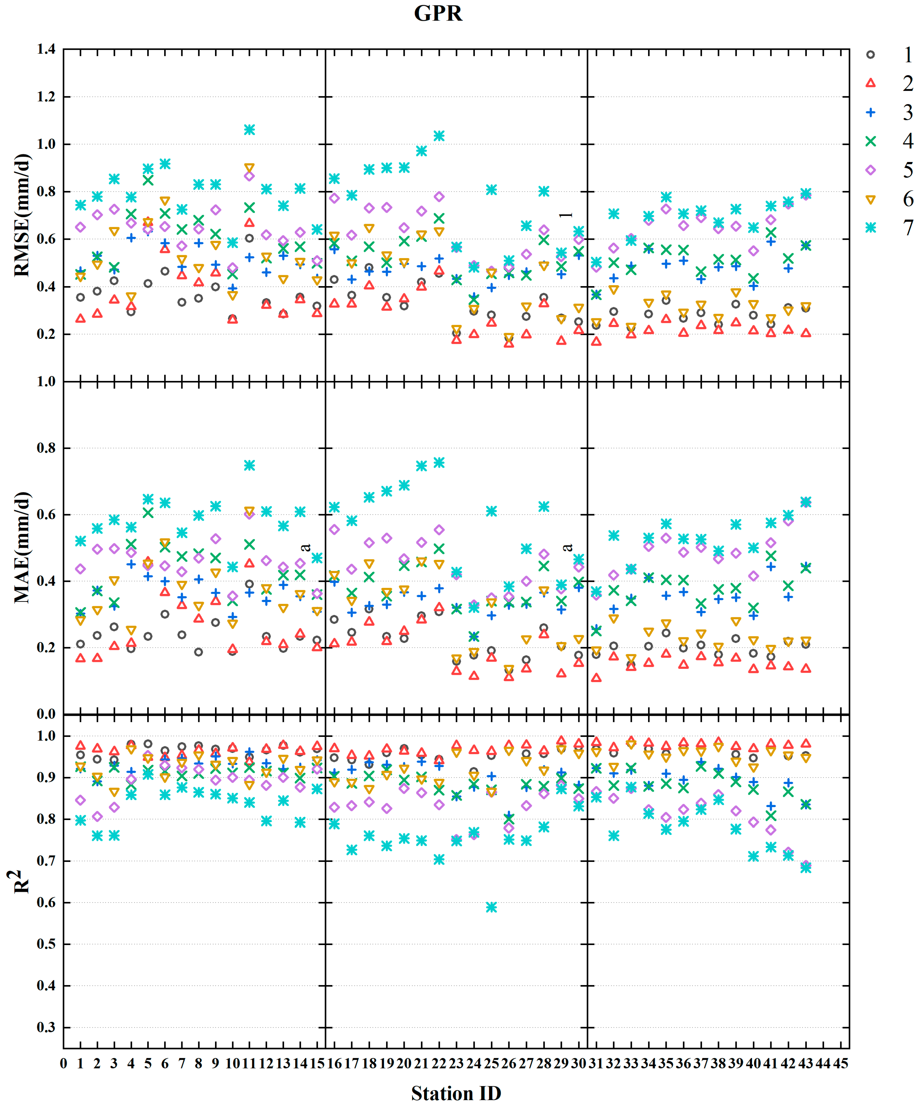
2.2.2. Gaussian Process Regression (GPR) Model

Rasmussen and Williams (2004) [45] defined GPR as a complex set of random variables with a joint Gaussian distribution. Kernel-based approaches can work together to solve flexible and applicable problems. Two functions are usually used to explain GPR: the mean and the covariance function. These are given by the following formulas:

$$\mathrm{f}\approx \mathit{GP}\left(m,k\right)$$

(4)

In the equation:

• $\mathit{f}$: the Gaussian distribution;
• $m$: the mean function;
• $k$: the covariance function.

The covariance value represents the correlation between the various outputs related to the input, and can determine the correlation between a single output and the input. The specific formula is as follows:

$$Cov\left(x_p\right)=C_f\left(x_p\right)+C_n\left(x_p\right)$$

(5)

In the equation:

• $C_f$: the functional part;
• $C_n$: the noise part of the system.

Gaussian process regression (GPR) is closely related to SVM, and is part of the kernel machine region in ML models. Kernel methods comprise sample-based learners. Instead of learning fixed parameters, the kernel remembers training data samples and assigns certain weights to them.

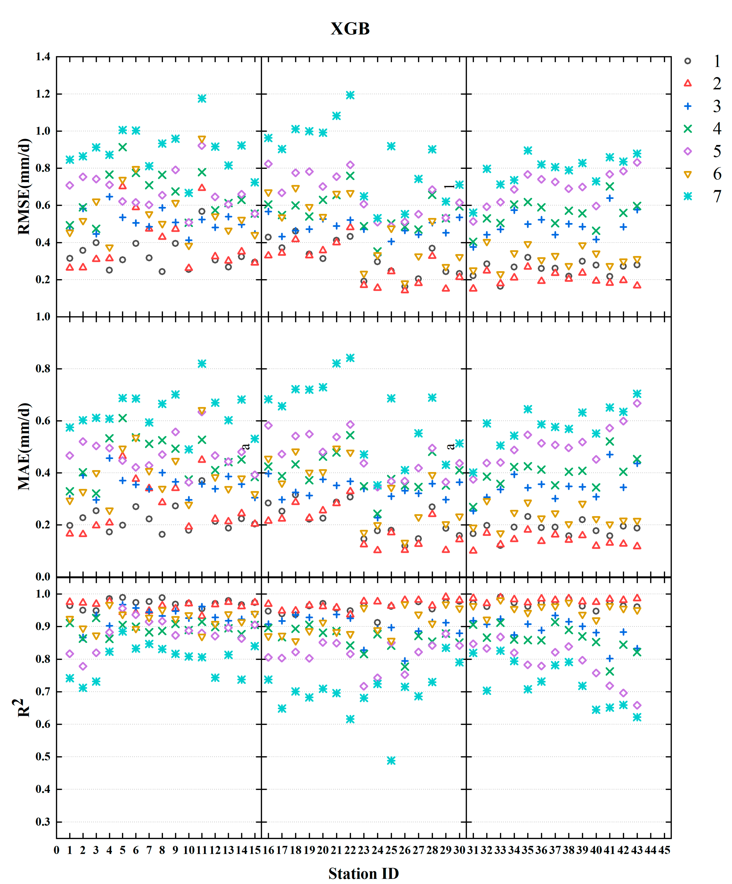
2.2.3. Extreme Gradient Boosting (XGBoost) Model

XGBoost is a new type of gradient boosting machine (GBM) that improves the handling of databases by optimizing the decision tree algorithm. It solves the overfitting problem through regularization and built-in cross-validation, improves computational accuracy, and maintains an optimal calculation speed. In addition, during the training period, the functions in the XGBoost model will be run and computed automatically, so they are widely used in feature extraction [46], classification [47] and estimation [48]. The XGBoost model is derived from “boosting,” which combines a set of predictions of all weak learners and trains strong learners through special training. Its formula is as follows:

$$f_i^{\left(t\right)}={\displaystyle \sum _{k=1}^t{f}_k}\left(x_i\right)=f_i^{\left(t-1\right)}+f_t\left(x_i\right)$$

(6)

In the equation:

$f_k\left(x_i\right)$ and $f_t\left(x_i\right)$: the predicted values of the $k$-th and $i$-th iterations of the XGBoost model;

$f_i^{\left(t\right)}$ and $f_i^{\left(t-1\right)}$: the predicted value of the $t$ and $t-1$ iterations of the $i$ sample;

$x_i$: the input variable ($k$ = [1,2,…,t], =[1,2,…,n]).

To prevent the overfitting problem without affecting the calculation speed of the model, the XGBoost model can derive the following formula:

$$Ob{j}^{\left(t\right)}={\displaystyle \sum _{i=1}^{n}l\left(f_i^{\left(\overline{t}\right)},f_i^{\left(t\right)}\right)}+{\displaystyle \sum _{i=1}^n\Omega \left(f_i\right)}$$

(7)

In the equation:

• $l$: the loss function;
• $Ob{j}^{\left(t\right)}$: the objective function;
• $f_i^{\left(\overline{t}\right)}$: the actual value of the $t$-th iteration of the $i$-th sample;
• $\Omega \left(f_i\right)$: the regular term of the objective function, whose equation is:

$$\Omega \left(f_i\right)=\beta T+\frac{1}{2}\lambda {\Vert \omega \Vert }^2$$

(8)

In the equation:

• $\beta$ and $\lambda$: regularization coefficients;
• $T$: the number of leaf nodes.

In terms of adjusting the parameters of these models, grid search method is used in XGB model. The presented statistical parameters (R², RMSE and MAE) are trained with 70% of the data, and the remaining 30% are verified. As for the machine learning model, this paper applies the same model to all stations.

2.2.4. Inputs of Meteorological Parameters

In this study, first of all, when the meteorological station data are missing, the CLDAS data are used to replace them, and eight different input combinations are set (the CLD subscripts represent the CLDAS data). When one measured meteorological factor is missing, combination 1 (T_max·T_min·R_s·U₂·RH_CLD), combination 2 (T_max·T_min·R_s·U_2CLD·RH) and combination 3 (T_max·T_min·R_sCLD·U₂·RH) are set. When two measured meteorological factors are missing, combination 4 (T_max·T_min·R_sCLD·U_2CLD·RH), combination 5 (T_max·T_min·R_sCLD·U₂·RH_CLD) and combination 6 (T_max·T_min·R_s·U_2CLD·RH_CLD) are set. When there are only temperature data, combination 7 (T_max·T_min·R_sCLD·U_2CLD·RH_CLD) is set. When all measured data are missing, combination 8 (T_maxCLD·T_minCLD·R_sCLD·U_2CLD·RH_CLD) is set. The input combination corresponding to the machine learning method is shown in

Table 3. Eight input combinations set by PM-CLDAS method and machine learning method according to missing data.

Input	CLDAS	GPR	XGB
	Combination	Combination
1	Tmax·Tmin·Rs·U2·RHCLD	Tmax·Tmin·Rs·U2
2	Tmax·Tmin·Rs·U2CLD·RH	Tmax·Tmin·Rs·RH
3	Tmax·Tmin·RsCLD·U2·RH	Tmax·Tmin·U2·RH
4	Tmax·Tmin·RsCLD·U2CLD·RH	Tmax·Tmin·RH
5	Tmax·Tmin·RsCLD·U2·RHCLD	Tmax·Tmin·U2
6	Tmax·Tmin·Rs·U2CLD·RHCLD	Tmax·Tmin·Rs
7	Tmax·Tmin·RsCLD·U2CLD·RHCLD	Tmax·Tmin
8	TmaxCLD·TminCLD·RsCLD·U2CLD·RHCLD	-

.

2.2.5. Statistical Indicators

Quantitative measures, including the coefficient of determination ($R^2$), root-mean-square error ($RMSE$) and mean absolute error ($MAE$), were used to evaluate the performance of the different combinations in estimating daily $E{T}_0$, as follows:

$$R^2=\frac{{\left[{{\displaystyle \sum }}_{i=1}^n\left(E{T}_{0i}-{\stackrel{-}{ET}}_{0i}\right)\left(E{T}_{0CLDi}-{\stackrel{-}{ET}}_{0CLDi}\right)\right]}^2}{{{\displaystyle \sum }}_{i=1}^n{(E{T}_{0i}-{\stackrel{-}{ET}}_{0i})}^2{{\displaystyle \sum }}_{i=1}^n{(E{T}_{0CLDi}-{\stackrel{-}{ET}}_{0CLDi})}^2}$$

(9)

$$RMSE=\sqrt{\frac{1}{n}{\displaystyle \sum }_{i=1}^n{\left(E{T}_{0i}-E{T}_{0CLDi}{}_i\right)}^2}$$

(10)

$$MAE=\frac{1}{n}{\displaystyle \sum }_{i=1}^n\left|E{T}_{0i}-E{T}_{0CLDi}\right|$$

(11)

In the equations:

$E{T}_{0i}$: the ET₀ calculated using meteorological station data;

$E{T}_{0CLDi}$: the ET₀ calculated using the CLDAS data;

${\stackrel{-}{ET}}_{0i}$: the average ET₀ calculated using meteorological station data;

${\stackrel{-}{ET}}_{0CLDi}$: the average ET₀ calculated using the CLDAS data;

$n$: the number corresponding to ET₀ data.

Higher R² values (closer to 1) or lower RMSE and MAE values indicate a better estimation performance of the CLDAS dataset.

3. Results

3.1. Estimation When One Type of Meteorological Data Is Missing

When the meteorological station data are relatively complete and the calculation of ET₀ lacks certain data except for temperature, the estimation performances of the three methods under combinations 1, 2, and 3 are shown in

Table 4. The PM–CLDAS method and two machine learning methods estimate the performance of ET₀ under combinations 1, 2, and 3.

Input/	RMSE mm/d	MAE mm/d	R2
Model
1
CLDAS	0.312	0.217	0.966
GPR	0.330	0.223	0.961
XGB	0.303	0.210	0.966
2
CLDAS	0.377	0.248	0.969
GPR	0.303	0.208	0.968
XGB	0.301	0.205	0.968
3
CLDAS	0.661	0.424	0.838
GPR	0.488	0.351	0.911
XGB	0.493	0.345	0.907

. Better performances are shown in bold (all the statistical parameters displayed here are the average values of the statistical parameters calculated for each site).

Under combination 1, when local meteorological RH data are missing, the CLDAS data RH_CLD are used to replace them to estimate ET₀. The three methods perform well, and the XGB method has good accuracy (R² = 0.966, RMSE = 0.303 mm/d, and MAE = 0.210 mm/d). The performance of the PM–CLDAS method is second, and the performance of the GPR method is relatively poor.

Under combination 2, when the local meteorological U₂ data are missing, the CLDAS data U_2CLD are used to replace them to estimate ET₀. The results calculated using the three methods have good correlation with the measured data (R² > 0.968), and the CLDAS performs relatively poorly in terms of RMSE and MAE (RMSE = 0.377 mm/d, and MAE = 0.248 mm/d).

Under combination 3, when the local meteorological R_s data are missing, the CLDAS data R_sCLD are used to replace them to estimate ET₀. The estimation performance drops significantly relative to combinations 1 and 2, and the PM–CLDAS method performs relatively poorly (R² = 0.838, RMSE = 0.661 mm/d, and MAE = 0.424 mm/d).

Overall, when we use the CLDAS data RH_CLD or U_2CLD instead of the measured data to estimate ET₀, accuracy and stability are high. However, when there is a lack of local meteorological R_s data, the estimated results drop significantly (by about 5%~13.5%), but there is still a certain degree of accuracy. Therefore, the accuracy of the CLDAS R_sCLD data is relatively low [39], which affects the estimation of ET₀. These results are similar to the results reported by Liu et al. (2009) [49] and Fan et al. (2019) [50]. This may be due to the immature radiation simulation mechanism of the CLDAS and the severe air pollution in the areas mentioned above, which pose certain challenges in respect of obtaining accurate simulations [18]. Therefore, we propose using the corresponding CLDAS data instead of local meteorological data to predict ET₀ when the local meteorological RH or U₂ data are missing; when the Rs data are missing, we can use machine learning methods to predict ET₀. Furthermore, we selected three meteorological stations in different climate zones and compared the ET₀ estimated by the three methods with the measured ET₀, as shown in Figure 2. It can still be found that the scattered points of combination 1 and combination 2 are more concentrated, and the estimate for combination 3 is even worse.

3.2. Estimation When Two Kinds of Meteorological Data Are Missing

When the data from the meteorological stations are relatively scarce, and the calculation of ET₀ lacks two kinds of data except temperature, the estimation performances of the three methods under combinations 4, 5, and 6 are shown in

Table 5. The PM–CLDAS method and two machine learning methods estimate the performance of ET₀ under combinations 4, 5 and 6.

Input/	RMSE mm/d	MAE mm/d	R2
Model
4
CLDAS	0.768	0.531	0.786
GPR	0.546	0.399	0.892
XGB	0.592	0.419	0.874
5
CLDAS	0.802	0.539	0.761
GPR	0.638	0.465	0.846
XGB	0.673	0.481	0.828
6
CLDAS	0.477	0.302	0.947
GPR	0.438	0.312	0.932
XGB	0.458	0.322	0.925

, and the better performances are shown in bold.

Under combination 4, when the local R_s and U₂ data are missing, and the CLDAS R_sCLD and U_2CLD data are used to replace them to estimate ET₀, the performance of the three methods decreases compared to the case where only one type of meteorological data is missing. The performance of the XGB and GPR methods is relatively better (R² > 0.874, RMSE < 0.592 mm/d, and MAE < 0.419 mm/d), but the performance of the PM–CLDAS method drops significantly (R² = 0.786). Under combination 5, when the local R_s and RH data are missing, and the CLDAS R_sCLD and RH_CLD data are used to replace them to estimate ET₀, the specific situation is the same as in combination 4. The performance of the XGB and GPR methods is relatively good (R² > 0.828), and the performance of the PM–CLDAS method has a significant decline (R² = 0.761). However, under combination 6, when the local U₂ and RH data are missing, and the CLDAS U_2CLD and RH_CLD data are used to replace them to estimate ET₀, the estimated performance is significantly improved compared to combinations 4 and 5, and second only to combinations 1 and 2. The PM–CLDAS method performs relatively well (R² = 0.947, RMSE = 0.477 mm/d, and MAE = 0.302 mm/d).

Overall, when we use CLDAS RH_CLD and U_2CLD data instead of local meteorological data to estimate ET₀, accuracy and stability are high. However, when the missing data involve R_s, the estimation results drop significantly (about 3.5%~19.6%) but still have accuracy. It can still be concluded that the accuracy of the CLDAS R_sCLD data is relatively low, which affects the estimation of ET₀, so we suggest that when local meteorological RH and U₂ data are missing, the corresponding CLDAS data are used instead to estimate ET₀. We also suggest using machine learning methods to estimate ET₀ when the lack of data involves R_s. Furthermore, we selected three meteorological stations in different climate zones and compared the ET₀ estimated using the three methods with the measured ET₀, as shown in Figure 3. It can still be found that the scattered points of combination 4 and combination 5 are more concentrated, and the estimate for combination 6 is even better.

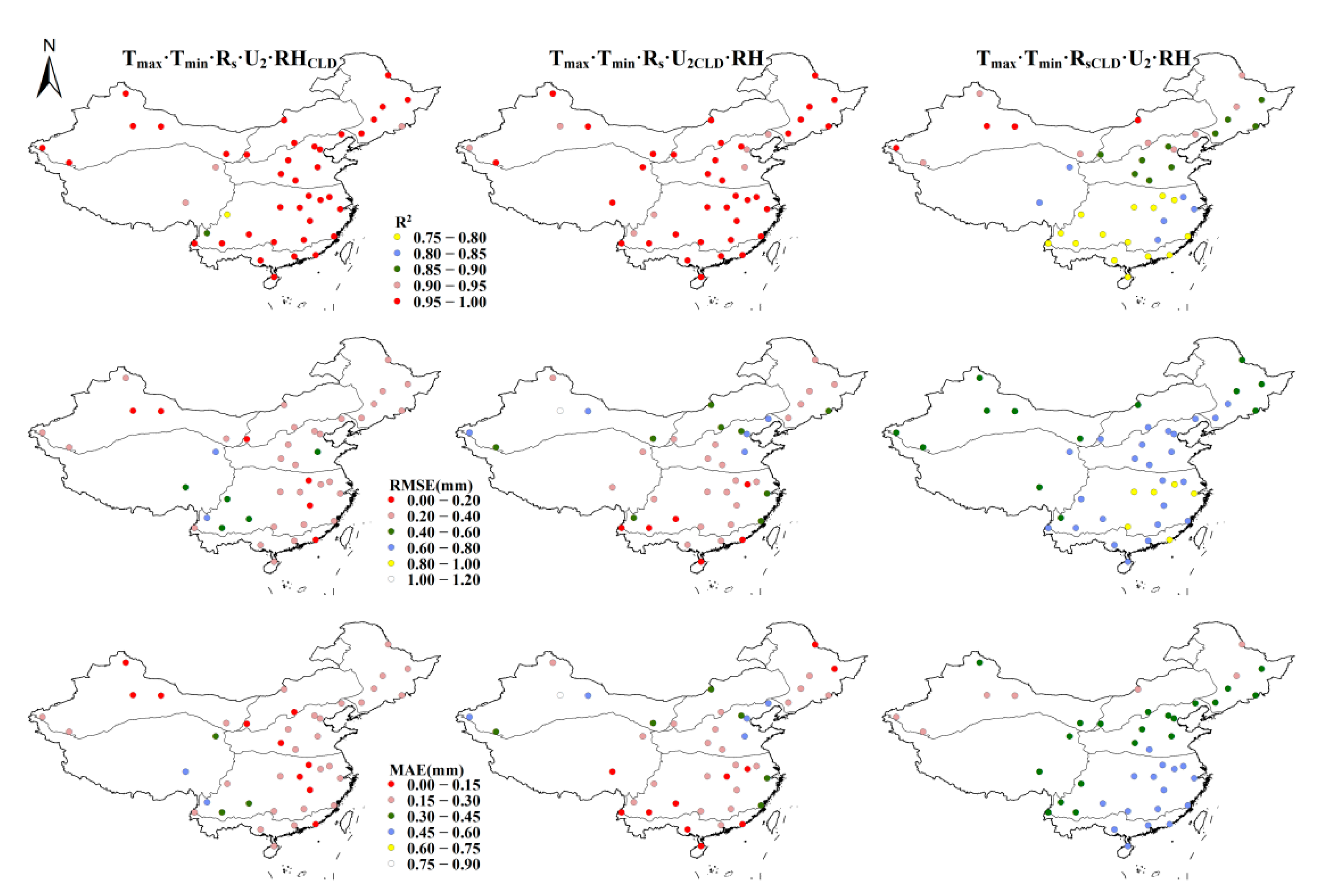
3.3. Estimation When Three Kinds of Meteorological Data Are Missing

When the meteorological station data are very scarce, and the calculation of ET₀ only involves the temperature data, the estimation performances of the three methods under combination 7 are shown in

Table 6. The PM–CLDAS method and two machine learning methods estimate the performance of ET₀ under combination 7.

Input/	RMSE mm/d	MAE mm/d	R2
Model
7
CLDAS	0.860	0.601	0.740
GPR	0.753	0.559	0.791
XGB	0.848	0.614	0.741

, and the better performances are shown in bold.

Under combination 7, when the local R_s, U₂ and RH data are missing, and the CLDAS R_sCLD, U_2CLD and RH_CLD data are used to replace them to estimate ET₀, the performance of the three methods decreases compared to the case where two meteorological data types are missing. The performance of the XGB (R² = 0.741) and CLDAS (R² = 0.740) methods is relatively worse. The GPR method performs better (R² = 0.791, RMSE = 0.753 mm/d, and MAE = 0.559 mm/d). Compared to combination 4, the estimated performance of the three methods decreases by about 5% under combination 7. Therefore, we propose the use of the machine learning method GPR to estimate ET₀ when only temperature data are available. In addition, we selected three stations and compared their estimated ET₀ with the measured ET₀, as shown in Figure 4.

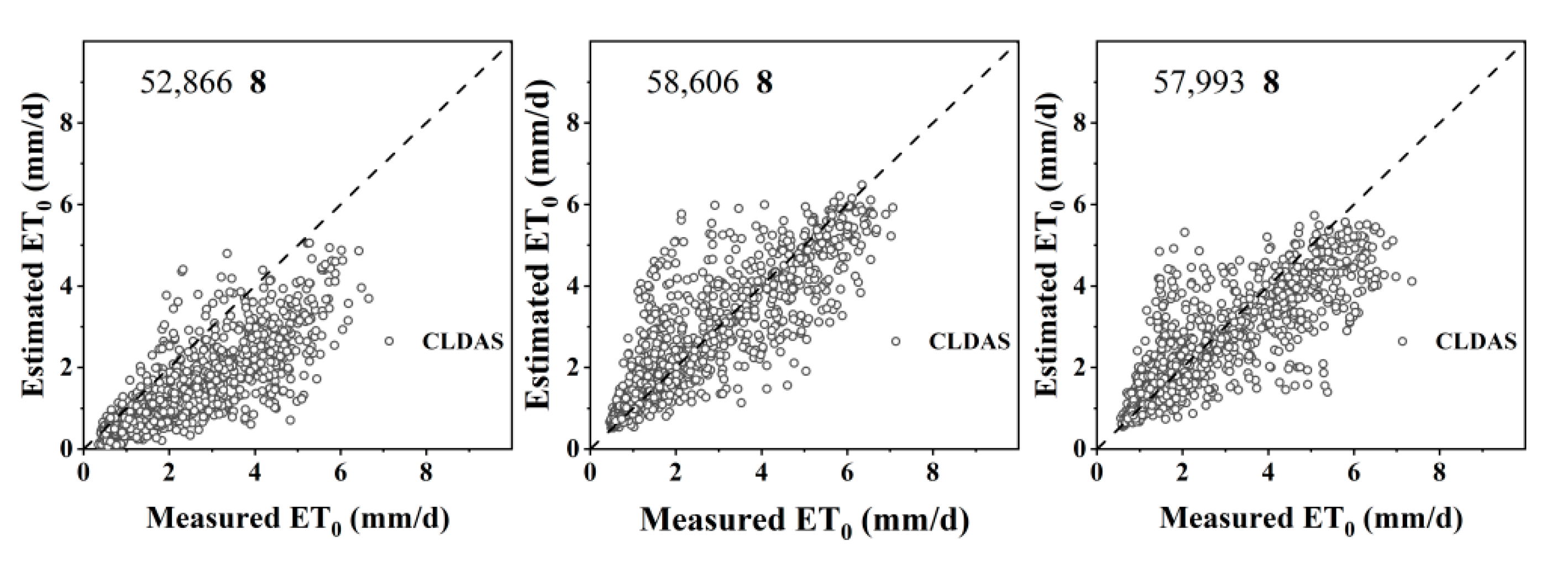
3.4. Estimation When All Meteorological Data Are Missing

In the actual situation, there are no meteorological stations in some areas. When the data for all meteorological factors are unavailable, the performance of estimating ET₀ is shown in

Table 7. The PM–CLDAS method and two machine learning methods estimate the performance of ET₀ under combination 8.

Input/	RMSE mm/d	MAE mm/d	R2
Model
8
CLDAS	0.963	0.678	0.701

. As can be seen from the table, when all CLDAS data are used instead, the performance is slightly lower than that of combination 7, but the overall performance is still good.

Overall, when we replace local meteorological data with CLDAS R_sCLD, U_2CLD and RH_CLD data to estimate ET₀, combination 7 (R² = 0.740, RMSE = 0.860 mm/d, and MAE = 0.601 mm/d) does not result in a significant decline in the accuracy of estimating ET₀ compared to combinations 4 and 5, but the estimated stability declines to a certain extent; therefore, combination 7 represents a dataset with a high-cost performance. When we use all CLDAS data to estimate ET₀, the results show that combination 8 (R² = 0.701, RMSE = 0.963 mm/d, and MAE = 0.678 mm/d) is not far behind combination 7; considering the difficulty in obtaining ET₀ using this method, the results of combination 8 to estimate ET₀ are entirely acceptable. Combination 8 is especially suitable for those areas where there are no weather stations temporarily. In addition, we selected three stations and compared their estimated ET₀ with the measured ET₀, as shown in Figure 5. All the statistical indicators of ET₀ estimated using the PM–CLDAS method and machine learning methods under different combinations are shown in Figure 6, Figure 7 and Figure 8.

3.5. Estimation by the PM–CLDAS Method in Different Climate Zones

When the data from the meteorological stations are relatively complete, and only one of the data types except temperature is missing, the PM–CLDAS method is used to calculate ET₀. The estimated ET₀ in the seven climate zones is shown in

Table 8. The PM–CLDAS method estimates the performance of ET₀ in seven climate zones under combinations 1, 2, and 3.

Zone	Tmax·Tmin·Rs·U2·RHCLD			Tmax·Tmin·Rs·U2CLD·RH			Tmax·Tmin·RsCLD·U2·RH
	RMSE mm/d	MAE mm/d	R2	RMSE mm/d	MAE mm/d	R2	RMSE mm/d	MAE mm/d	R2
Ⅰ	0.257	0.167	0.989	0.652	0.430	0.949	0.488	0.287	0.954
Ⅱ	0.263	0.161	0.985	0.431	0.275	0.966	0.578	0.328	0.918
Ⅲ	0.311	0.205	0.965	0.331	0.192	0.968	0.565	0.324	0.892
Ⅳ	0.305	0.204	0.974	0.508	0.351	0.949	0.688	0.417	0.884
Ⅴ	0.330	0.241	0.955	0.276	0.185	0.975	0.751	0.511	0.772
Ⅵ	0.241	0.178	0.973	0.206	0.132	0.982	0.768	0.560	0.694
Ⅶ	0.589	0.440	0.920	0.243	0.163	0.974	0.603	0.381	0.830
average	0.312	0.217	0.966	0.377	0.248	0.969	0.661	0.424	0.838

.

For combination 1 (T_max·T_min·R_s·U₂·RH_CLD), after replacing the missing local meteorological RH data with the CLDAS RH_CLD data, the PM–CLDAS performed better in zones 1–6 (R² > 0.955, RMSE < 0.330 mm/d, and MAE < 0.241 mm/d). Zone 7 was the next-best performer (R² = 0.920, RMSE = 0.589, and MAE = 0.440), and the overall performance in the seven zones was better (R² = 0.966). For combination 2 (T_max·T_min·R_s·U_2CLD·RH), after replacing the missing local meteorological U₂ data with the CLDAS U_2CLD data, the performance in all seven zones was good (R² = 0.969). It was the best in zone 6 (R² = 0.982) and the worst in zone 1 (R² = 0.949). For combination 3 (T_max·T_min·R_sCLD·U₂·RH), after replacing the missing local meteorological R_s data with the CLDAS R_sCLD data, the best performance was in zones 1 and 2 (R² > 0.918), followed by zones 3 and 4, and there was a relatively poor performance in the remaining zones 5–7 (R² < 0.830, RMSE > 0.603 mm/d, and MAE > 0.381 mm/d). The specific performance is shown in Figure 9.

When the data from meteorological stations are relatively scarce (two meteorological variables are missing), the performance of their estimated ET₀ in the seven climate zones is shown in

Table 9. The PM–CLDAS method estimates the performance of ET₀ in seven climate zones under combinations 4, 5, and 6.

Zone	Tmax·Tmin·RsCLD·U2CLD·RH			Tmax·Tmin·RsCLD·U2·RHCLD			Tmax·Tmin·Rs·U2CLD·RHCLD
	RMSE mm/d	MAE mm/d	R2	RMSE mm/d	MAE mm/d	R2	RMSE mm/d	MAE mm/d	R2
Ⅰ	0.762	0.509	0.914	0.628	0.393	0.926	0.737	0.504	0.940
Ⅱ	0.702	0.457	0.884	0.722	0.431	0.879	0.486	0.329	0.951
Ⅲ	0.659	0.429	0.851	0.738	0.466	0.815	0.443	0.289	0.940
Ⅳ	0.811	0.568	0.820	0.824	0.529	0.824	0.566	0.408	0.936
Ⅴ	0.812	0.570	0.710	0.875	0.611	0.671	0.387	0.294	0.955
Ⅵ	0.813	0.605	0.644	0.875	0.658	0.608	0.279	0.203	0.967
Ⅶ	0.645	0.445	0.800	0.871	0.620	0.695	0.542	0.452	0.938
average	0.768	0.531	0.786	0.802	0.539	0.761	0.477	0.302	0.947

.

For combination 4 (T_max·T_min·R_s·U_2CLD·RH_CLD), after replacing missing local meteorological U₂ and RH data with the CLDAS U_2CLD and RH_CLD data, there was a better performance in zones 1–3 (R2 > 0.851, RMSE < 0.762 mm/d, and MAE < 0.509 mm/d), and a poor performance in zones 4~7 (R² < 0.820, RMSE > 0.645 mm/d, MAE > 0.445 mm/d). The best performance was in zones 1 and 2 (R² < 0.884) and the worst performance was in zone 6 (R² = 0.644); overall, there was a mediocre performance in estimating ET₀ in the seven zones (average R² = 0.786). For combination 5 (T_max·T_min·R_sCLD·U₂·RH_CLD), after replacing the missing local meteorological R_s and RH data with the CLDAS R_sCLD and RH_CLD data, the performance in zones 1 and 2 was good (R² > 0.879), the performance in regions 3~7 was relatively average (R² < 0.824, RMSE > 0.738 mm/d, and MAE > 0.466 mm/d), and the worst performance was in zone 6 (R² = 0.608). For combination 6 (T_max·T_min·R_s·U_2CLD·RH_CLD), after replacing the missing local meteorological U₂ and RH data with the CLDAS U_2CLD and RH_CLD data, the overall performance was good (R² = 0.947, RMSE = 0.477 mm/d, and MAE = 0.342 mm/d). The specific performance is shown in Figure 10.

When the data from meteorological stations are very scarce, we set up two combinations. The performance of their estimated ET₀ in the seven climate zones is shown in

Table 10. The PM–CLDAS method estimates the performance of ET₀ in seven climate zones under combinations 7 and 8.

Zone	Tmax·Tmin·RsCLD·U2CLD·RHCLD			TmaxCLD·TminCLD·RsCLD·U2CLD·RHCLD
	RMSE mm/d	MAE mm/d	R2	RMSE mm/d	MAE mm/d	R2
Ⅰ	0.880	0.592	0.888	0.984	0.669	0.863
Ⅱ	0.797	0.522	0.853	0.918	0.600	0.810
Ⅲ	0.789	0.523	0.791	0.895	0.594	0.738
Ⅳ	0.889	0.621	0.783	0.978	0.683	0.742
Ⅴ	0.878	0.624	0.661	0.977	0.702	0.612
Ⅵ	0.880	0.665	0.588	0.936	0.704	0.546
Ⅶ	0.832	0.613	0.716	1.069	0.834	0.678
average	0.860	0.601	0.740	0.963	0.678	0.701

.

For combination 7 (T_max·T_min·R_sCLD·U_2CLD·RH_CLD), after replacing the missing local meteorological R_s, U₂, and RH data with the CLDAS R_sCLD, U_2CLD, and RH_CLD data, there was a relatively good performance in zones 1 and 2 (R² > 0.853), an average performance in zones 3 (R² = 0.791) and 4 (R² = 0.783), and a poor and unstable performance in zones 5–7 (R² < 0.716, RMSE > 0.832, and MAE > 0.613), in which zone 6 performed the worst. Combination 7 performed poorly in estimating ET₀ in the seven climate zones, with a significant drop in accuracy and stability compared to when lacking two local meteorological data types. For combination 8 (T_maxCLD·T_minCLD·R_sCLD·U_2CLD·RH_CLD), after replacing all the missing local meteorological data with all the CLDAS data, the performance in zones 1 and 2 was relatively good (R² > 0.810), and the performance in zones 3 (R² = 0.738) and 4 (R² = 0.742) was relatively average. The performance in regions 5~7 was significantly reduced (R² <0.678, RMSE > 0.936 mm/d, and MAE > 0.704 mm/d). The specific performance is shown in Figure 11.

4. Discussion

In this study, we found that the accuracy of ET₀ is very sensitive to the amount of data, which is similar to the findings of Ni et al. (2019) [51] et al.; its accuracy will decrease with the decrease in the number of input parameters. The reason for this phenomenon is that the XGBoost model uses a greedy algorithm. When the input data are not sufficient to explain the cause of all evaporation changes, the model will over-explain to a certain extent. The GPR model has higher requirements for data distribution. When the data distribution does not conform to the Gaussian distribution, the accuracy of the model will be affected. Therefore, the GPR model is not recommended as the prediction model for this region. In addition, the accuracy of each method is higher when the four meteorological factors T_max, T_min, RH and U₂ are input, and the results are similar to those of Cao et al. (2011) [52] and Mao et al. (2020) [4]. On the whole, ET₀ is positively sensitive to changes in air temperature, wind speed and solar radiation, and negatively sensitive to changes in relative humidity. Among these, ET₀ is the most sensitive to solar radiation [25], followed by relative humidity and 2 m wind speed, and ET₀ is the least sensitive to temperature changes. In addition, the modeling of global wind speed has always been challenging and often difficult to predict. Similar results have been obtained in reanalysis data, such as the ERA5 [53], NCEP/NCAR [30] and GLDAS [54]. This may be because the terrain change in some areas is very complex, and the roughness of the underlying surface will also challenge the prediction of wind speed. In addition, the prediction of the wind speed direction is very difficult [18]. Solar radiation is an important parameter of the ET₀ radiation term, which usually has a great impact on ET₀ [55,56]. Finally, Liu et al. [57] analyzed the cause of reference crop evapotranspiration in the Yunnan Guizhou Plateau, and the results show that solar radiation has the greatest effect on ET₀ at an annual scale.

As far as the results of estimating ET₀ are concerned, the overall results for the CLDAS are good, especially for air temperature data; these results are the same as those of Liu et al. (2021) [32], but the estimation accuracy is not as good as the machine learning methods in some cases. This is due to the instability of the accuracy of the CLDAS R_sCLD data [18], which has a particularly negative impact on the results when estimating ET₀; subsequent bias correction can be performed on the CLDAS data, which may improve the prediction results [58]. However, in the current situation, we do not recommend using the CLDAS data instead of local meteorological R_s data.

China’s administrative regions are divided into four levels: provinces, cities, counties and towns, of which the province is the highest level of administrative division. Various provinces/autonomous regions have formulated many relevant policies based on climate change, and these policies also have differences [59]. Therefore, separately controlling the data quality of the CLDAS from the perspective of each province will better improve the accuracy of the CLDAS data, which can help different provinces/autonomous regions select and apply the CLDAS data sets according to their own needs. At the same time, the division of provinces/autonomous regions in China is mostly based on natural geographical attributes, such as mountains and rivers, which are closely related to the division of climate [60]. Therefore, it is important to evaluate the dataset on a province-wide basis, provide a more detailed reference basis from an application point of view, and consider different types of environmental climate.

When using the CLDAS near-surface meteorological data to estimate ET₀, it is generally reliable in the plain area of China but has large fluctuations in complex terrain areas and high-altitude areas under some input combinations [61]. Overall, some individual stations have relatively high errors when they are located at high altitudes, in areas with complex terrain, and in areas with sparse observations. These stations are often located in areas with a complex topography and significant elevation changes, which can lead to problems with the representativeness of the stations (the Digital Terrain Model (DTM) map (elevation and slope) of the Qinghai–Tibet Plateau is shown in Figure 12); thus, more caution is required when using data from these areas [62,63]. However, we only assessed gridded datasets for a limited time and a limited number of meteorological stations, which may not accurately demonstrate the assessed characteristics of some climate states. In addition, the evaluation results of high-altitude stations are relatively poor. Therefore, how to correct the evaluation results of these stations, in addition to increasing the number of research stations, is a problem that needs further research.

We evaluated the performance of the CLDAS dataset in estimating ET₀ across China during the period 2017–2020. Not only the Penman–Monteith method but also other methods and different datasets can be used to calculate ET₀. Weiland et al. (2012) [64] compared six different methods using Climate Forecast System Reanalysis (CFSR) data and evaluated the results with Global Climate Research Unit (CRU) data, pointing out that the PM method was data-intensive and sensitive to inaccuracies in the input data. Five complete meteorological factors were required to calculate ET₀ and the estimation accuracy decreased with a decline in the number of input climatic factors; therefore, the recalibrated Hargreaves equation was recommended. Lang et al. (2017) [65] compared eight models in southwest China with the PM method and found that the Makkink and the Hargreaves–Samani methods can be good alternatives to the PM method. Therefore, the Hargreaves method has advantages in regions such as Africa, where the complete datasets of climatic variables are generally inaccessible [66].

5. Conclusions

In this study, we evaluated which of the CLDAS product or machine learning simplified model is more suitable to estimate ET₀ when meteorological data are insufficient in China. According to the number of missing meteorological data, eight combinations were set for comparative analysis. The results show the following.

In the case of missing meteorological data, where local meteorological U₂ or RH data are missing, it is recommended that U_2CLD or RH_CLD data from the CLDAS products are used to replace the data of the local meteorological station to estimate ET₀. When the R_s data are missing, the performance estimated by the PM–CLDAS method degrades significantly, and it is recommended that machine learning is used to estimate ET₀. Therefore, among the CLADS products, R_sCLD significantly affects the estimation accuracy of ET₀.

When two kinds of data, except temperature data, are missing, the performance of the three methods in estimating ET₀ decreases to varying degrees. Furthermore, we propose to use the corresponding CLDAS data instead of local meteorological data to estimate ET₀ in the absence of meteorological RH and U₂ data. Nevertheless, when the lack of data involves R_s, it is recommended that machine learning methods are used to estimate ET₀.

When multiple meteorological factor data are missing, it is recommended that machine learning methods are used to estimate ET₀ when there are only local temperature data. In addition, when all data are missing, it is recommended that the CLDAS data are used instead of local meteorological data to estimate ET₀, which estimation performance is acceptable.

In addition, we analyzed the estimation performance of the PM–CLDAS method in seven regions under different combinations. We concluded that the performance in zones 1–5 is relatively good, and the performance in zones 6~7 may fluctuate. To summarize, when the CLDAS data are used to estimate ET₀, the calculation results for T_maxCLD, T_minCLD, RH_CLD and U_2CLD are more accurate. However, the use of R_sCLD needs careful consideration in some zones.

References

1. Cui, Y.; Jia, L.; Fan, W. Estimation of actual evapotranspiration and its components in an irrigated area by integrating the Shuttleworth-Wallace and surface temperature-vegetation index schemes using the particle swarm optimization algorithm. Agric. For. Meteorol. 2021, 307, 108488. [Google Scholar] [CrossRef]
2. Zuo, D.P.; Xu, Z.X.; Li, J.Y.; Liu, Z.F. Spatiotem poral characteristics of potential evapotranspiration in the Weihe River basin under future climate change. Adv. Water Sci. 2011, 22, 455–461. [Google Scholar]
3. Huang, Y.C.; Cui, N.B.; Chen, X.Q.; Xu, H.R.; Zhang, Y.X. Simulation of Reference Crop Evapotranspiration in the Hilly Area of Central Sichuan Based on Different Machine Learning Models. China Rural. Water Hydropower 2020, 5, 13–20, 27. [Google Scholar] [CrossRef]
4. Mao, Y.P.; Fang, S.F. Research of Reference Evapotranspiration’s Simulation based on Machine Learning. J. Geo-Inf. Sci. 2020, 22, 1692–1701. [Google Scholar] [CrossRef]
5. Tabari, H.; Kisi, O.; Ezani, A.; Hosseinzadeh Talaee, P. SVM, ANFIS, regression and climate based models for reference evapotranspiration modeling using limited climatic data in a semi-arid highland environment. J. Hydrol. 2012, 444, 78–89. [Google Scholar] [CrossRef]
6. Wu, L.F.; Fan, J.L. Comparison of neuron-based, kernel-based, tree-based and curve-based machine learning models for predicting daily reference evapotranspiration. PLoS ONE 2019, 14, e0217520. [Google Scholar] [CrossRef] [Green Version]
7. Feng, Y.; Cui, N.B.; Gong, D.; Zhang, Q.; Zhao, L. Evaluation of random forests and generalized regression neural networks for daily reference evapotranspiration modelling. Agric. Water Manag. 2017, 193, 163–173. [Google Scholar] [CrossRef]
8. Huang, G.; Wu, L.; Ma, X.; Zhang, W.; Fan, J.; Yu, X.; Zhou, H. Evaluation of CatBoost method for prediction of reference evapotranspiration in humid regions. J. Hydrol. 2019, 574, 1029–1041. [Google Scholar] [CrossRef]
9. Liu, X.Q.; Dai, Z.G.; Wu, L.F.; Zhang, F.C.; Dong, J.H. Comparing the Performance of GPR, XGBoost and CatBoost Models for Calculating Reference Crop Evapotranspiration in Jiangxi Province. J. Irrig. Drain. 2021, 40, 91–96. [Google Scholar] [CrossRef]
10. Wang, S.; Fu, Z.; Ding, Y.; Wu, L.; Wang, K. Simulation of reference evapotranspiration based on random forest method. Trans. Chin. Soc. Agric. Mach. 2017, 48, 302–309. [Google Scholar] [CrossRef]
11. Zhang, H.J.; Cui, N.B.; Xu, Y.; Zhong, D.; Hu, X.T.; Gong, D.Z. Prediction for reference crop evapotranspiration in arid northwest China based on ELM. J. Drain. Irrig. Mach. Eng. 2018, 36, 779–784. [Google Scholar] [CrossRef]
12. Feng, Y.; Peng, Y.; Cui, N.; Gong, D.; Zhang, K. Modeling reference evapotranspiration using extreme learning machine and generalized regression neural network only with temperature data. Comput. Electron. Agric. 2017, 136, 71–78. [Google Scholar] [CrossRef]
13. Thongkao, S.; Ditthakit, P.; Pinthong, S.; Salaeh, N.; Elkhrachy, I.; Linh, N.T.T.; Pham, Q.B. Estimating FAO Blaney-Criddle b-Factor Using Soft Computing Models. Atmosphere 2022, 13. [Google Scholar] [CrossRef]
14. Ferreira, L.B.; da Cunha, F.F.; de Oliveira, R.A.; Filho, E.I.F. Estimation of reference evapotranspiration in Brazil with limited meteorological data using ANN and SVM–A new approach. J. Hydrol. 2019, 572, 556–570. [Google Scholar] [CrossRef]
15. Bakhtiari, B.; Mohebbi, D.A.; Qaderi, K. Estimation of daily reference evapotranspiration with limited meteorological data in selected Iran’s semi-arid climates. Iran-Water Resour. Res. 2016, 3, 131–144. [Google Scholar]
16. Chia, M.Y.; Huang, Y.F.; Koo, C.H. Reference evapotranspiration estimation using adaptive neuro-fuzzy inference system with limited meteorological data. In IOP Conference Series: Earth and Environmental Science, Proceedings of the 6th International Conference on Water Resource and Environment, Online Conference, 23–26 August 2020; IOP Publishing: Bristol, UK, 2020; Volume 612, p. 012017. [Google Scholar] [CrossRef]
17. Mahto, S.S.; Mishra, V. Does ERA-5 outperform other reanalysis products for hydrologic applications in India. J. Geophys. Res. Atmos. 2019, 124, 9423–9441. [Google Scholar] [CrossRef]
18. Wu, L.F.; Qian, L.; Huang, G.M.; Liu, X.G.; Wang, Y.C.; Bai, H.; Wu, S.F. Assessment of Daily of Reference Evapotranspiration Using CLDAS Product in Different Climate Regions of China. Water 2022, 14, 1744. [Google Scholar] [CrossRef]
19. Sheffield, J.; Goteti, G.; Wood, E.F. Development of a 50-year high-resolution global dataset of meteorological forcings for land surface modeling. J. Clim. 2006, 19, 3088–3111. [Google Scholar] [CrossRef] [Green Version]
20. Sheffield, J.; Ziegler, A.D.; Wood, E.F.; Chen, Y. Correction of the high-latitude rain day anomaly in the NCEP–NCAR reanalysis for land surface hydrological modeling. J. Clim. 2004, 17, 3814–3828. [Google Scholar] [CrossRef]
21. Srivastava, P.K.; Han, D.; Ramirez, M.A.R.; Islam, T. Comparative assessment of evapotranspiration derived from NCEP and ECMWF global datasets through Weather Research and Forecasting model. Atmos. Sci. Lett. 2013, 28, 4419–4432. [Google Scholar] [CrossRef]
22. Hwang, S.; Graham, W.D.; Geurink, J.S.; Adams, A. Hydrologic implications of errors in bias-corrected regional reanalysis data for west central Florida. J. Hydrol. 2014, 510, 513–529. [Google Scholar] [CrossRef]
23. Woldesenbet, T.; Elagib, N. Spatial-temporal evaluation of different reference evapotranspiration methods based on the climate forecast system reanalysis data. Hydrol. Process. 2016, 35, e14239. [Google Scholar] [CrossRef]
24. Srivastava, P.K.; Han, D.; Islam, T.; Petropoulos, G.P.; Gupta, M.; Dai, Q. Seasonal evaluation of evapotranspiration fluxes from MODIS satellite and mesoscale model downscaled global reanalysis datasets. Theor. Appl. Climatol. 2015, 124, 461–473. [Google Scholar] [CrossRef]
25. Pelosi, A.; Terribile, F.; D’Urso, G.; Chirico, G.B. Comparison of ERA5-Land and UERRA MESCAN-SURFEX reanalysis data with spatially interpolated weather observations for the regional assessment of reference evapotranspiration. Water 2020, 12, 1669. [Google Scholar] [CrossRef]
26. Tian, D.; Martinez, C.J. Forecasting Reference Evapotranspiration Using Retrospective Forecast Analogs in the Southeastern United States. J. Hydrometeorol. 2012, 13, 1874–1892. [Google Scholar] [CrossRef]
27. Song, Y.; Su, X.L.; Niu, J.P.; Cui, C.F. Temporal and spatial characteristics and forecasting of reference crop evaporation in Shaanxi. J. Northwest A F Univ.—Nat. Sci. Ed. 2015, 43, 225–234. [Google Scholar] [CrossRef]
28. Liu, Z.; Lu, J.; Huang, J.; Chen, X.; Zhang, L.; Sheng, Y. Prediction and trend of future reference crop evapotranspiration in the Poyang Lake Basin based on CMIP5 Models. J. Lake Sci. 2019, 31, 1685–1697. [Google Scholar]
29. Martins, D.S.; Paredes, P.; Raziei, T.; Pires, C.; Cadima, J.; Pereira, L.S. Assessing reference evapotranspiration estimation from reanalysis weather products. An application to the Iberian Peninsula. Int. J. Climatol. 2016, 37, 2378–2397. [Google Scholar] [CrossRef]
30. Raziei, T.; Parehkar, A. Performance evaluation of NCEP/NCAR reanalysis blended with observation-based datasets for estimating reference evapotranspiration across Iran. Theor. Appl. Climatol. 2021, 144, 885–903. [Google Scholar] [CrossRef]
31. Milad, N.; Mehdi, H. Reference crop evapotranspiration for data-sparse regions using reanalysis products—ScienceDirect. Agric. Water Manag. 2022, 262, 107319. [Google Scholar] [CrossRef]
32. Liu, Y.; Shi, C.X.; Wang, H.J.; Han, S. Applicability assessment of CLDAS temperature data in China. Trans. Atmos. Sci. 2021, 44, 540–548. [Google Scholar] [CrossRef]
33. Shi, C.X.; Pan, Y.; Gu, J.X.; Xu, B.; Han, S.; Zhu, Z.; Zhang, L. A review of multi-source meteorological data fusion products. Acta Meteorol. Sin. 2019, 77, 774–783. [Google Scholar] [CrossRef]
34. Xia, Y.; Hao, Z.; Shi, C.; Li, Y.; Meng, J.; Xu, T.; Wu, X.; Zhang, B. Regional and global land data assimilation systems: Innovations, challenges, and prospects. J. Meteorol. Res. 2019, 33, 159–189. [Google Scholar] [CrossRef]
35. Han, S.; Shi, C.X.; Jiang, L.P.; Zhao, T.; Jiang, Z.W.; Xu, B.; Li, X.F.; Zhu, Z.; Lin, H.J. The Simulation and Evaluation of Soil Moisture Based on CLDAS. J. Appl. Meteorol. Sci. 2017, 28, 369–378. [Google Scholar] [CrossRef]
36. Shan, S.; Shi, C.X.; Shen, R.P.; Bai, L. Evaluation of EAR70, CLDAS, and ERA-Interim Reanalysis Surface Soil Temperatures Across China. Meteorol. Sci. Technol. 2021, 49, 830–837. [Google Scholar] [CrossRef]
37. Wang, H.Y.; Wu, X.P.; Liu, K.L.; Liu, Y.Q. Spatial and temporal variation of land surface temperature in Taklamakan desert. Hubei Agric. Sci. 2022, 61, 152–159. [Google Scholar] [CrossRef]
38. Wang, H.; Huang, J.; Zhou, H.; Zhao, L.; Yuan, Y. An integrated variational mode decomposition and arima model to forecast air temperature. Sustainability 2019, 11, 4018. [Google Scholar] [CrossRef] [Green Version]
39. Huang, X.L.; Han, S.; Shi, C.X. Multiscale Assessments of Three Reanalysis Temperature Data Systems over China. Agriculture 2021, 11, 1292. [Google Scholar] [CrossRef]
40. Allen, R.G.; Pereira, L.S.; Raes, D.; Smith, M. Crop Evapotranspiration—Guidelines for Computing Crop Water Requirements, Irrigation and Drain—FAO Irrigation and Drainage; Paper No. 56; FAO: Rome, Italy, 1998. [Google Scholar]
41. Holman, D.; Sridharan, M.; Gowda, P.; Porter, D.; Marek, T.; Howell, T.; Moorhead, J. Gaussian process models for reference ET estimation from alternative meteorological data sources. J. Hydrol. 2014, 517, 28–35. [Google Scholar] [CrossRef]
42. Karbasi, M. Forecasting of multi-step ahead reference evapotranspiration using wavelet- Gaussian process regression model. Water Resour. Management. 2018, 32, 1035–1052. [Google Scholar] [CrossRef]
43. Chen, Z.Y.; Wu, L.F.; Liu, X.Q.; Wu, Z.R.; Dong, J.H. Prediction of pan evaporation of Jiangxi Province using GPR, CatBoost and XGBoost models. J. Water Resour. Water Eng. 2020, 11. [Google Scholar] [CrossRef]
44. Niu, M.L.; Li, H.; Li, X.X. A CatBoost Model for Simulating the Daily Reference Evapotranspiration in Greenhouse. Water Sav. Irrig. 2022, 1, 16–19. [Google Scholar] [CrossRef]
45. Williams, C.K.; Rasmussen, C.E. Gaussian Processes for Machine Learning (Adaptive Computation and Machine Learning). Int. J. Neural Syst. 2004, 14, 69–106. [Google Scholar] [CrossRef] [Green Version]
46. Jiang, S.F.; Wu, T.J.; Peng, X.; Li, J.Q.; Li, Z.; Sun, T. Data Driven Fault Diagnosis Method Based on XGBoost Feature Extraction. China Mech. Eng. 2020, 31, 8. [Google Scholar] [CrossRef]
47. Xu, Y.; Zhen, J.N.; Jiang, X.P.; Wang, J.J. Mangrove species classification with UAV-based remote sensingdata and XGBoost. Natl. Remote Sens. Bull. 2021, 25, 737–752. [Google Scholar] [CrossRef]
48. Guo, Y.L.; Li, L.T.; Chen, W.Q.; Cui, J.Q.; Wang, Y.L. Research on the Estimation of Winter Wheat Chlorophyll Content Based on Red Edge Spectral and XGBoost Algorithm. Infrared 2020, 41, 11. [Google Scholar] [CrossRef]
49. Liu, X.; Mei, X.; Li, Y.; Wang, Q.; Jensen, J.R.; Zhang, Y.; Porter, J.R. Evaluation of temperature-based global solar radiation models in China. Agric. For. Meteorol. 2009, 149, 1433–1446. [Google Scholar] [CrossRef]
50. Fan, J.; Wu, L.; Zhang, F.; Cai, H.; Zeng, W.; Wang, X. Empirical and machine learning models for predicting daily globalsolar radiation from sunshine duration: A review and case study in China. Renew. Sustain. Energy Rev. 2019, 100, 186–212. [Google Scholar] [CrossRef]
51. Ni, N.Q.; Li, G.; Cui, N.B.; Jiang, S.Z.; Tang, Q.; Liu, S.M.; Liao, G.L.; Wang, L.T. Sensitivity Analysis of Reference Crop Evapotranspiration in Southwest China in Recent 56 Years. Jiangsu Agric. Sci. 2019, 20, 298–305. [Google Scholar] [CrossRef]
52. Cao, W.; Shen, S.H.; Duan, C.F. Sensitivity Analysis of the Reference Crop Evapotranspiration during Growing Season in the Northwest China in Recent 49 Years. Chinese J. Agrometeorol. 2011, 32, 375–381. [Google Scholar] [CrossRef]
53. Li, T.J.; Cao, H.X. Research of the sensitivity of the reference crop evapotranspiration to main meteorological factors in the Guanzhong region. J. Northwest AF Univ. 2009, 37, 68–74. [Google Scholar]
54. Blankenau, P.A.; Kilic, A.; Allen, R. An evaluation of gridded weather data sets for the purpose of estimating reference evapotranspiration in the United States. Agric. Water Manag. 2020, 242, 106376. [Google Scholar] [CrossRef]
55. Petković, B.; Petković, D.; Kuzman, B. Neuro-fuzzy estimation of reference crop evapotranspiration by neuro fuzzy logic based on weather conditions. Comput. Electron. Agric. 2020, 173, 105358. [Google Scholar] [CrossRef]
56. Xia, X.S.; Zhu, X.F.; Pan, Y.Z. Influence of solar radiation empirical values on reference crop evapotranspiration calculation in different regions of China. Trans. Chin. Soc. Agric. Mach. 2020, 51, 254–266. [Google Scholar] [CrossRef]
57. Liu, Q.S.; Wu, Z.J.; Cui, N.B. Spatial-temporal distribution characteristics and attribution analysis of reference crop evapotranspiration in Yunnan-Kweichow Plateau. J. Drain. Irrig. Mach. Eng. 2022, 40, 302–310. [Google Scholar] [CrossRef]
58. Dong, C.Q.; Guo, Y.Y.; Zhang, L.; Hu, J.Y. Deviation Correction Method of Grid Temperature Prediction Based on CLDAS Data. J. Arid. Meteorol. 2021, 39, 847–856. [Google Scholar] [CrossRef]
59. Wang, D.L.; Yu, Q. Structural Adjustment of State Spaces: Functional Transformation and Change Logic of Administrative Division in China in the Past 70 Years. Adm. Trib. 2019, 26, 5–12. [Google Scholar] [CrossRef]
60. Zhao, B.; Wang, K.Y.; Wang, F.Y.; Liu, H.M. The characteristics and changing trend of administrative boundary above county level in China. Geogr. Res. 2021, 40, 2494–2507. [Google Scholar] [CrossRef]
61. Chen, F.; Yang, X.; Ji, C.; Li, Y.; Deng, F. Establishment and assessment of hourly high-resolution gridded air temperature data sets in Zhejiang, China. Meteorol. Appl. 2019, 26, 396–408. [Google Scholar] [CrossRef] [Green Version]
62. Mobilia, M.; Longobardi, A. Prediction of Potential and Actual Evapotranspiration Fluxes Using Six Meteorological Data-Based Approaches for a Range of Climate and Land Cover Types. Int. J. Geo-Inf. 2021, 70, 192. [Google Scholar] [CrossRef]
63. Huo, Z.L.; Shi, H.B.; Chen, Y.X.; Wei, Z.M.; Qu, Z.Y. Spatio-temporal variation and dependence analysis of ET0 in north arid and cold region. Trans. Chin. Soc. Agric. Eng. 2004, 6, 60–63. [Google Scholar] [CrossRef]
64. Weiland, F.C.S.; Tisseuil, C.; Durr, H.H.; Vrac, M.; Beek, L.P.H. Selecting the optimal method to calculate daily global reference potential evaporation from CFSR reanalysis data for application in a hydrological model study. Hydrol. Earth Syst. Sci. 2012, 16, 983–1000. [Google Scholar] [CrossRef] [Green Version]
65. Lang, D.; Zheng, J.; Shi, J.; Liao, F.; Ma, X.; Wang, W.; Zhang, M. A comparative study of potential evapotranspiration estimation by eight methods with FAO Penman–Monteith method in southwestern China. Water 2017, 9, 734. [Google Scholar] [CrossRef]
66. Trambauer, P.; Dutra, E.; Maskey, S.; Werner, M.; Pappenberger, F.; Beek, L.P.H.; Uhlenbrook, S. Comparison of different evaporation estimates over the African continent. Hydrol. Earth Syst. Sci. Discuss. 2014, 18, 193–212. [Google Scholar] [CrossRef]
Figure 1. Geographical distribution of 43 meteorological stations.
Sustainability 14 14577 g001
Figure 2. Comparison of the estimated ET0 and the measured ET0 of the three methods under combinations 1, 2, and 3.
Sustainability 14 14577 g002
Figure 3. Comparison of the estimated ET0 and the measured ET0 of the three methods under combinations 4, 5, and 6.
Sustainability 14 14577 g003
Figure 4. Comparison of the estimated ET0 and the measured ET0 of the three methods under combination 7.
Sustainability 14 14577 g004
Figure 5. Comparison of the estimated ET0 and the measured ET0 of the three methods under combination 8.
Sustainability 14 14577 g005
Figure 6. Statistical index of estimating ET0 using the XGB method under different combinations.
Sustainability 14 14577 g006
Figure 7. Statistical index of estimating ET0 using the GPR method under different combinations.
Sustainability 14 14577 g007
Figure 8. Statistical index of estimating ET0 using the PM–CLDAS method under different combinations.
Sustainability 14 14577 g008
Figure 9. The spatial distribution of estimated ET0 performance under combinations 1, 2, and 3.
Sustainability 14 14577 g009
Figure 10. The spatial distribution of estimated ET0 performance under combinations 4, 5, and 6.
Sustainability 14 14577 g010
Figure 11. The spatial distribution of estimated ET0 performance under combinations 7 and 8.
Sustainability 14 14577 g011
Figure 12. The DTM map (elevation and slope) of the Qinghai–Tibet Plateau.
Sustainability 14 14577 g012