Econometric Approaches That Consider Farmers’ Adaptation in Estimating the Impacts of Climate Change on Agriculture: A Review

Abstract

The question of whether and to what extent farmers can adapt to climate change has recently gained academic interest. This paper reviews contemporary econometric approaches that assess the impacts of climate change on agriculture and consider farmer adaptation, complementing previous methodological reviews with this distinctive adaptation perspective. The value of adaptation can be measured by comparing the differences between the long-term climate change effect and the short-term weather shock effect. However, this theoretical model has not yet been well supported by empirical evidence, as it is difficult to identify true adaptation, incorporating adaptation cost, and estimated adaptation rate. Quasi-natural experiments, cost-benefit analysis, and Bayesian models are effective tools to address these methodological drawbacks. Two methods dominate in the estimation of climate effects, but each has its own advantages. A good estimate provides a trade-off between the incorporation of farmers’ adaptive behavior and the reduction in omitted variables bias. Cross-sectional data models based on climate variability can capture farmers’ long-term adaptations but are prone to bias due to omitted variables. Panel data models are more effective at mitigating omitted variable bias by applying fixed effects, but do not consider farmers’ adaptative behavior to long-term climate change. To address this dilemma, several cutting-edge approaches have been developed, including integration with the weather and climate model, the long differences approach, and the long- and short-term hybrid approach. We found three key challenges, namely: (1) exploring adaptation mechanisms, (2) the CO₂ fertilization effect, and (3) estimating the distributional effects of climate impacts. We also recommend future empirical studies to incorporate satellite remote sensing data, examine the relationship between different adaptation measures, model farmers’ future climate expectations, and include adaptation costs.

1. Introduction

Over the last two decades, econometric methods have become increasingly popular in estimations of climate change’s impacts on agriculture [1,2,3,4,5,6,7]. However, previous studies have adopted numerous climatic indicators and the consequent impacts on agriculture vary considerably. For example, the projected impacts range from severe damage [2] to slightly positive effects [1]. Researchers widely acknowledge that the discrepancies in these findings largely depend on the extent of farmers’ adaptation to climate change [8,9]. Adaptation enriches theoretical and policy studies by clarifying the implications of climate change if adaptation occurs. Some adaptation measures may require large investments that farmers cannot afford. If the benefits of adaptation are fewer than the costs of adaptation, then the best option for farmers is to avoid the adjustment (Figure 1) [10]. In this case, the continued use of suboptimal farming methods may lead to future profit losses [9]. Thus, exploring the value of adaptation may inspire governments to weigh the costs and benefits of supporting adaptation activities.

Process-based crop models are widely used to simulate how crops grow in interaction with the environment and can provide reliable quantitative information about the effects of changing climatic factors on crop yields. Crop modes examine the effects of climatic factors on crop yields by precisely controlling all the elements required for crop growth (temperature, humidity, light, soil, fertilizer, etc.) in the simulation experiment [11]. The econometric approach uses a large amount of historical data to examine the relationship between climatic factors and agricultural production, while controlling for technological progress, economic factors and climate adaptation behavior [12]. The econometric approach assumes that, if agricultural production is profitable, rational farmers will take adaptive measures, such as changing land use and increasing irrigation inputs, to take full advantage of favorable climate resources and avoid unfavorable climate conditions. Compared to crop models, econometric studies may reach conclusions that are closer to the real world because they consider farmers’ adaptive behavior [13].

One of the most frequently used econometric approaches is the Ricardian method, introduced by Mendelsohn et al. [1], which relies on cross-sectional variation to measure the impacts of climate change on farmland productivity. The identification of long-term impacts arises from the assumption that farmers seek to maximize their agricultural outcomes under a certain climate and that each farmer should have enough time to adapt to a changing climate. A number of empirical results stemming from Ricardian model applications indicate that adaptation is influential and can even completely reverse the negative effects of warming on agriculture [13]. However, contrary to these findings, some evidence from emerging econometric approaches, such as panel data and long differences models, suggests that farmers do not adequately adapt to climate change [2,4,14]. The divergence between these empirical studies arises from the diverse model settings and the extent of adaptation that they can account for. Although the Ricardian model can analyze farmers’ long-term adaptation, it is susceptible to omitted variable bias (biased estimates of the adaptation value) [14]. The panel data and long differences models have control over unobservable omitted variables, but the identified adaptation measures can only be implemented in the short- or medium-term, thus effectively moderating the adverse effects of unanticipated weather shocks [9]. Using the envelope theorem, Hsiang [15] argues that panel data models can estimate long-term climate responses, as the value of long-term adaptation to climate change is zero. However, his model relies on some unrealistic assumptions: (1) agents always maximize profits, (2) climate change is stationary, (3) adaptation is continuous, and (4) adaptation has no associated costs.

In this context, the extent of farmers’ adaptation to climate change remains an empirical question that requires further methodological developments. First, the current models imply that the agricultural adaptation mechanism remains unchanged over time, and do not pay attention to the impact of agricultural structure transformation and agricultural technology progress. Second, the long differences model and Ricardian model estimate the total effects of all adaptation channels, but these approaches generally provide little information on how different adaptation types and levels play a role in mitigating the harmful, or exploiting the beneficial, effects of climate change. Third, in the analysis of the Ricardian model, product and factor prices are not directly controlled. Studies have shown that both product and factor prices are quite sensitive to climate shocks. Neglecting the role of prices will lead to biased results in the estimated climate impacts. Incorporating the Ricardian model into a general equilibrium model would provide a solution to this problem.

Several pieces of the literature have reviewed the quantification mechanisms of climate change’s impact using econometric approaches. For example, Ortiz-Bobea [16] provides an overview of the mixed statistical and biophysical approaches on modeling planting and harvesting decisions, irrigation and other input adjustments. Blanc and Schlenker [17] summarize the methodology of panel data model for estimating the impacts of climate change on crop yields or agriculture productivity. Kolstad and Moore [9] conduct an in-depth review with an emphasis on the costs of adaptation, which will depend on the rate of adaptation and the effectiveness of adaptation options. However, few studies provide a comprehensive overview of econometric approaches for estimating the impact of climate change under farmers’ adaptation and identify the knowledge gaps and future model development in this field.

The aim of this paper is to explore the major econometric approaches that integrated farmer adaptation, in terms of their strengths and weaknesses, to highlight the knowledge gaps and potential future model developments. We analyze the theoretical specification differences emerging in these approaches to determine why inconsistencies occurred in previous empirical results. This paper will contribute to a better understanding of the mechanisms involved in climate modeling for agricultural adaptation and provide researchers with an overview of state-of-the-art methodological tools, and its findings provide lessons for research on climate change adaptation in other fields.

The rest of this paper is organized as follows. In Section 2, we present a review approach. In Section 3, we establish a conceptual framework to model farmer adaptation. In Section 3, we review the econometric approaches to estimate the impact of climate change that consider farmer adaptation. In Section 4, we highlight the typical challenges in the analysis of climate–agriculture relationships and how to overcome them. Section 5 comprises the conclusions and key recommendations.

2. Review Approach

To explore the role of adaptation in estimating the climate’s impacts on agriculture, we performed a selective literature review. Papers included in our review had to meet the following criteria: (1) use classical econometric models (time series, cross-sectional and panel data models) to quantify the value of adaptation; (2) pioneer or improve econometric methodologies for quantifying the value of adaptation, rather than just applying the current model to a case; (3) have a high number of citations to ensure the reliability of methodology.

We first searched selected Web of Science databases for papers published within the last 30 years using the following keyword pairings: “climate change”, “agriculture”, “adaptation”, “impact”. These searches yielded a total of 3756 articles (Figure 2). Based on titles, we removed articles that were not addressing climate adaptation or that were not using econometric approaches. From the 456 articles remaining, we searched abstracts and removed papers that clearly did not meet our inclusion criteria (e.g., papers use classical econometric models (cross-sectional or panel data models) to quantify the value of adaptation), reducing the total to 397. From these, we removed those that did not meet all inclusion criteria defined above, based on a full reading. The search and exclusion process left us with 25 articles. Many articles were removed because they did not pioneer or improve methodologies for quantifying the value of adaptation, and merely focused on the application of econometric models. We displayed the evolution of econometric approaches that consider farmer adaptation in Figure 3.

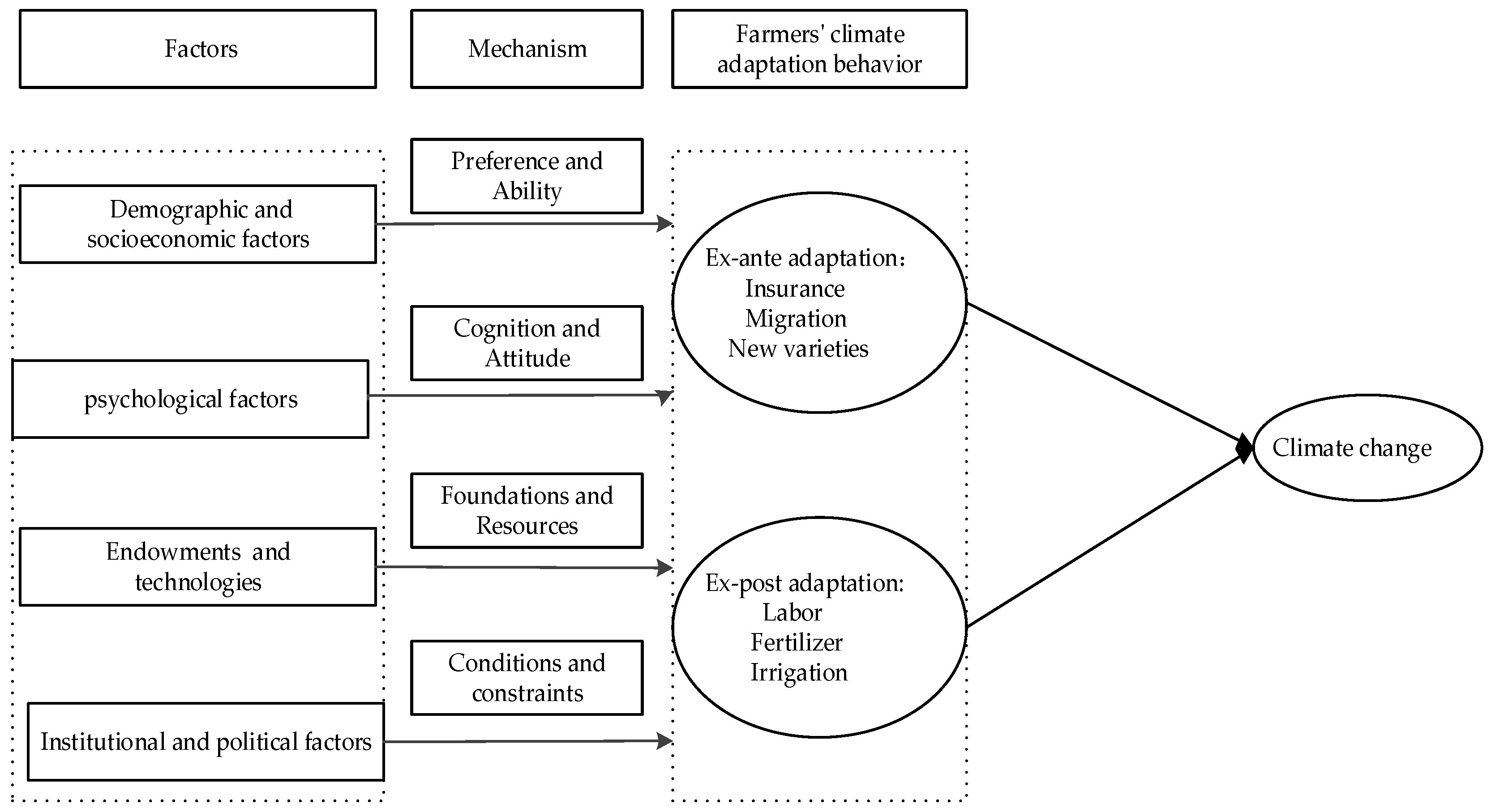
3. Conceptual Model of Climate Change Impacts on Agriculture Considering Farmer Adaptation

The econometric model used to estimate the impact of climate change on agriculture derives from the basic production function:

Y = f(X, Z).

Y: Agricultural output(ton).

X: a vector of climate-dependent choices including adaption choices and factor inputs, such as irrigation area(hectare) and fertilizer(kilogram).

Z: climate variables, such as temperature (°C) and precipitation(mm).

Assume that the prices of output Y and X are P and W, respectively; then, the profit π derived from producing agricultural product Y is:

π = P∙f [X, Z] − W∙X.

π: profit (USD).

Z: climate variables, such as temperature (°C) and precipitation (mm).

X: a vector of adaption choices and factor inputs, such as irrigation area(hectare) and fertilizer(kilogram).

and fertilizer.

P and W: the price vector of output Q and choice variables X.

Adaptation to climate change involves “the process of making adjustments to the actual or expected climate and its effects, in order to moderate its harm or exploit beneficial opportunities [12]”. In economics, farmers’ choices of adaptive behavior will be a rational optimization process. That is, a farmer will choose the optimal set of adaptation measures and input levels that can maximize his or her profits given the local climate [1]. Specifically, the optimization process for a farmer is to maximize:

$$\underset{\mathrm{X}}{\max }\mathsf{\pi }=\mathrm{P}·f\left[\mathrm{X},\mathrm{Z}\right]-\mathrm{W}·\mathrm{X}$$

(1)

π: profit (USD).

Z: climate variables, such as temperature (Celsius degree) and precipitation(mm).

X: a vector of adaption choices and factor inputs, such as irrigation, varieties

and fertilizer.

P and W: the price vector of output Q and choice variables X.

The necessary condition for the optimal solution of Equation (1) is ∂π/∂X = 0. The optimal climate adaptation choices and factor inputs would be a function of climate and price:

X* = x (Z, P, W).

X*: the optimal adaption and factor inputs demand.

Z: climate variables.

P and W: the price vector of output Q and choice variables X.

Substituting Equation (4) into Equation (1), the resulting output would be a function of climate and price:

y* = f [P, W, Z].

y*: the maximum output.

X*: the optimal adaption and factor inputs choices.

Z: climate variables.

P and W: the price vector of output Q and choice variables X.

Figure 2 further illustrates the relation between climate and profit. Assuming that the functional relationship between climate and profit is an inverted U-shape [4], under the different climatic conditions Z1 and Z2, farmers have two different optimal adaptation choices, X1 and X2, respectively, corresponding to two different profit functions.

If the adaptation measure X1 is not adjusted, when climate changes from Z1 to Z2, the farmer’s profit decreases from V0 to V2. Farmers may react to climate changes by switching the adaptation measure from X1 to X2, and the profit will decrease from V0 to V1. Thus, adjustment to the optimal adaption choices can mitigate the V1-V2 of loss from climate change (Figure 4).

Given the above conceptual framework, the estimated climate effect under farmers’ adaptation should be V1-V2. Climate econometrics has developed three approaches to consider the benefits of adaptation (

Table 1. Main characteristics of economic methodology measuring the benefit of adaptation.

Economic Methodology	Climate Variables	Sociodemographic and Orographic Variables	Main Problem
Comparing the cross-sectional variations in outcomes in different climatic zones	Cross-sectional weather average	Per capita income Population density Longitude Latitude Slope Soil quality	Omitted variable bias, such as irrigation and price [13], Unable to analyze specific crops [18], Unable to consider climate prediction information [19]
Comparing responses of outcome variables to high-frequency weather variation with to low-frequency weather variation	Decade-to-decade weather variation	Fertilizer Machine Labor	Underestimating the adaptation effect if high-frequency weather variation already incorporates some degree of adaptation effect [10], Omitted variable bias, such as technology and price
Comparing estimates derived from high-frequency weather variations across subsamples with different period	Seasonal/annual realizations of weather	Irrigation area soil quality	Unable to quantify adaptation effects of specific strategies, Bias due to measurement errors in weather variables [17]

Source: [9,13].

). The first approach is to compare the cross-sectional variations in outcomes (e.g., yield and profit) in different climatic zones. The approach assumes that, to maximize the benefits, farmers will adjust their production strategies to fully adapt to their local climate [9]. For example, farmers in different climatic zones adopt different crop varieties. The benefits of adopting new varieties under different historical climatic conditions can be measured by comparing crop yields or profit in different climatic zones.

The second approach will directly compare the responses of outcome variables to short-term weather shocks with long-term, gradual climate change. As gradual climate change is relatively long-term and predictable, this leaves enough time for farmers to respond. However, as weather shocks are unforeseen and random in most cases, farmers have only a very limited choice of response measures [13,20].

The third approach will compare the outcomes derived from high-frequency weather variation across subsamples over different periods. This approach argues that if farmers’ adaptation techniques continue to improve, then the sensitivity of agriculture to extreme heat should decrease over time [2,21,22].

However, it is challenging to statistically measure adaptation to climate change. The first challenge is to identify actual adaptation measures. For instance, Lobell [23] points out that some agronomic practices aimed at enhancing productivity are misclassified as adaptation measures. As technology upgrades would lead to the same yield gains under both warming and non-warming conditions, this practice does not moderate the yield losses caused by climate change. Thus, failing to exclude misclassified agronomic practices may exaggerate farmers’ potential to mitigate negative climate change effects through adaptation. Nonetheless, it is difficult to distinguish adaptation measures from other agricultural management activities, as agricultural measures cover adaptation to climate change and can often address many agricultural issues [24]. The investigation of location-specific genuine adaptation practices is, therefore, essential to identify true adaptation. Specifically, the researcher should first investigate whether the farmers have perceived the change in the local climate. Then, the researcher should investigate the benefits of specific adaptation measures that farmers have taken. Finally, the researcher can conduct a quasi-natural experiment to compare the differential impact of adaptation on adapters and non-adapters.

The second challenge is accounting for adaptation costs. Adaptation measures are not free and may require unaffordable investments in some cases. For example, Jagnani et al. [25] found that smallholder farmers will not change their inputs to respond to climate change, because they have financial constraints and cannot afford the cost of adaptation. Additionally, incorporating private adaptation costs in an empirical study is difficult, because the macro-information on these costs is unavailable. The cost of adaptation at the farm level must be collected as thoroughly as possible in future studies. Once information on the cost of adaptation is available, researchers can use cost-benefit analysis to measure the economic value of specific adaptation measures.

The third challenge relates to estimations of the adaptation rate, determining climate damage and adjustment costs to a large extent. Low adaptation rates result in adjustment costs [26]. This rate depends on an updated understanding of climate change [27]. However, it is difficult to observe how farmers update their beliefs about unobserved and nonstationary climate. People use realizations of weather to infer whether the climate is changing. Kelly et al. [26] and Moore [27] suggest that Bayesian statistical models can model how people update their beliefs about climate change by using sequential weather observations.

The fourth challenge is that theoretical models lack a micro-level farmer perspective to understand the mechanisms of adaptation. An analysis of the micro-perspective requires for the differences among individual farmers and the differences in adaptation behavior to climate change to be distinguished. We summarize four main influencing factors from the farmer’s perspective in Figure 3. These factors also differ in their mechanisms of influence regarding farmers’ choices to adapt. Demographic and socio-economic factors mainly influence farmers’ adaptation behavior by affecting their preferences and abilities. For example, older farmers have extensive experience in farming. They hold a broad knowledge about climate change and may know the necessity of climate adaptation [28]. Female farmers prefer conservative practices, and they are less willing to adopt new adaptation technologies [29]. Education can increase the likelihood of taking adaptive measures, as it makes farmers receive timely information and learn about improved technologies [30]. Among the psychological factors, perception and awareness of climate change are prerequisites for their adaptive behavioral choices. The stronger the farmers’ perception and knowledge of climate change, the more prominent their adaptive behaviors [31]. Capital and technology represent the material base and resource conditions possessed by farmers’ households. The human and social capital of households can improve the likelihood of adaptation to climate change by improving farmers’ access to information and technology [30]. Institutional and political factors are the conditions and real constraints that farmers face in their production. Clear land property rights will motivate farm households to adopt adaptation strategies to cope with climate change. Land-owning farmers are more likely to adopt new technologies to cope with the negative impacts of drought than land-leaseholders [32]. Future research should collect long-term data at the farmer level and distinguish differences in climate change adaptation among farmers with different characteristics, such as gender and cultural differences (Figure 5).

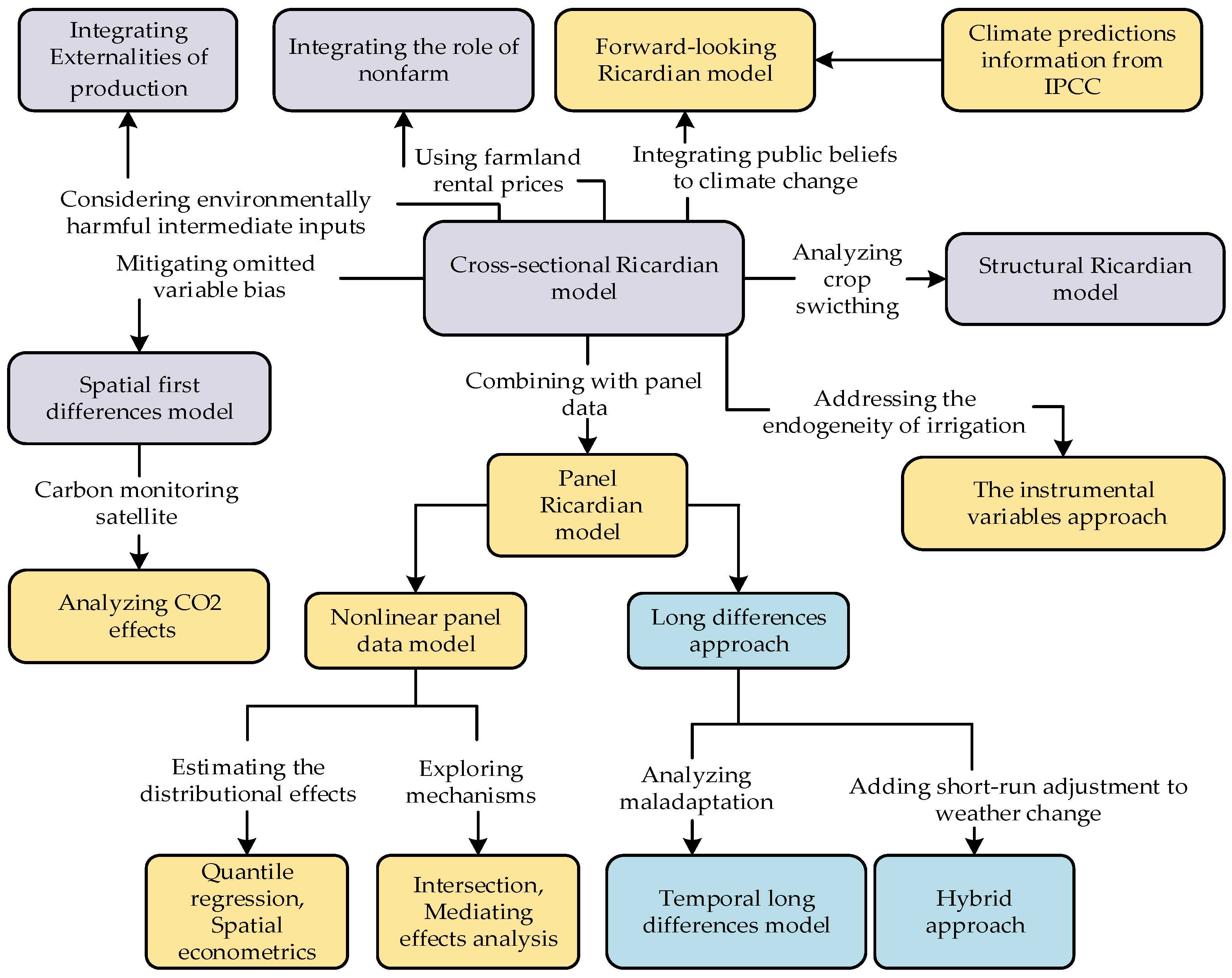
4. Econometric Approaches

Given the conceptual framework outlined above, short-term and long-term responses that depend on a specific setting are clearly all relevant to a full quantification of the role of adaptation. As various empirical methods describe the feasibility of estimating some or all of these responses, it is necessary to review some of the most common econometric approaches and the emerging techniques that combine short- and long-term variations in panel data to improve the quantification of climate change impacts (see

Table 2. Main characteristics of models quantifying the benefit of adaptation.

Model	Data	Crop Type	Adaptation	Environmental Conditions	Advantages	Disadvantages
Ricardian model	Land values, Long-term realizations of weather	No Specific crop	Long-term adaptation to climate change	Irrigation Soil quality No CO2 effects	Estimating long-term climate adaptation	Omitted variable bias Unable to consider price effects
Panel data model	Crop yields, farm profits, and total factor, seasonal/annual realizations of weather	Corn [2,3,4,33], Wheat [2,3], Cotton [2], Soybean [2,7,14], Barley [34], Banana [35]	Short-term to adaptation to weather change	CO2 effect Irrigation and soil quality are absorbed in the fixed effect	Estimating Short-term weather Adaptation, Robust to omitted variable bias	No long-term climate adaptation, Measurement errors in weather data
Hybrid approach	Crop yields, farm profits, and total factor, realizations of weather	Corn [4,20], Soybean [36], Barley [20]	Medium-term or long-term adaptation to climate change	Irrigation Soil quality No CO2 effect	Estimating long-term climate adaptation, Robust to Omitted variable bias	Unable to consider price effects, Unable to consider climate prediction information

Source: [9,13].

). Our examination of each technique involves an estimating equation, its ability to estimate adaptation, and its potential improvements.

4.1. Cross-Sectional Ricardian Model

Early studies exploit cross-sectional variations in average temperature and precipitation to estimate the long-term climate effects on agricultural outcomes across locations. For example, Mendelsohn et al. [1] propose a cross-sectional Ricardian model to determine the long-term equilibrium relationship between farmland value and climatic conditions. Their approach assumes that farmers adjust their cropping structure in response to local climate change to maximize profits. The adjustment benefits are eventually reflected in farmland value. Specifically, the cross-sectional Ricardian model can account for both intensive and extensive margin adaptation. It can be expressed as follows [1]:

$${\overline{\mathrm{V}}}_{it}=\mathsf{\alpha }+{\mathsf{\beta }\overline{\mathrm{Z}}}_{it}+{\mathsf{\gamma }\mathrm{X}}_{\mathrm{it}}+{\mathsf{\epsilon }}_{\mathrm{i}}$$

(2)

i: the location,

${\overline{\mathrm{V}}}_{it}$: the sum of the present value of land in the future,

${\overline{\mathrm{Z}}}_{it}$: the climate variables, including average temperature and average precipitation over the previous 30 years,

X: soil quality and socioeconomic variables,

ε_i: the error term,

α: the intercept term,

β: the marginal impacts of climate change,

γ: the marginal impacts of soil quality and socioeconomic variables.

A recent review shows that cross-sectional Ricardian studies examining climate impacts on agriculture have been carried out in over 40 countries [13]. Overall, it appears that, with a 2 °C increase in average global temperatures and a 7% increase in precipitation, Ricardian results predict an 8–12% decline in net farm revenue. The Ricardian approach has also been used to reveal that climate change impacts vary across regions. In this regard, warming benefits agriculture in cold regions, but undermines agriculture in warm regions.

Despite these advantages, the Ricardian model has the critical weakness of omitted variable bias. As the model cannot control some unobservable climate-related determinants of land value [13,18], various improvements were suggested to solve this problem. For instance, Massetti and Mendelsohn [37] adopted Hsiao’s two-step method to the Ricardian model, thus allowing for the estimation of climate impacts on farmland value to obtain both time-invariant (i.e., climate variables ${\overline{\mathrm{Z}}}_{it}$ in Equation (2)) and time-variant (i.e., control variable ${\mathrm{X}}_{\mathrm{it}}$ in Equation (1)) variables, using panel datasets. In the first stage, net revenue is regressed on time-varying variables by means of a fixed-effects method. In the second stage, the time-mean residuals obtained from the first stage are regressed on the climate variables. This approach mitigates omitted variable bias, because the fixed effects are controlled in the first stage.

Moreover, Drukenmiller and Hsiang [38] present the spatial first differences estimator to control the unknown omitted variables in the Ricardian model. This approach directly compares the outcomes in two neighboring counties. Intuitively, neighboring counties are more likely to share some characteristics, such as soil quality, farming system, and agricultural policy. By restricting comparisons to neighboring counties, this estimator can explicitly control for the omitted variable bias. The model can be expressed as [38]:

$${\mathrm{V}}_{\mathrm{i}}-{\mathrm{V}}_{\mathrm{i}-1}=\mathsf{\beta }\left({\mathrm{Z}}_{\mathrm{i}}-{\mathrm{Z}}_{\mathrm{i}-1}\right)+\mathsf{\gamma }\left({\mathrm{X}}_{\mathrm{i}}-{\mathrm{X}}_{\mathrm{i}-1}\right)+\left({\mathsf{\epsilon }}_{\mathrm{i}}-{\mathsf{\epsilon }}_{\mathrm{i}-1}\right)$$

(3)

i and i − 1: the observations that are immediately adjacent to one another,

V: the sum of the present value of land in the future,

Z: the climate variables, including average temperature and average precipitation over 30 years,

X: the soil quality and socioeconomic variables,

ε_i: the error term,

β: the marginal impacts of climate change,

γ: measures the marginal impacts of soil quality and socioeconomic variables.

The spatial first differences model is effective in identifying neighboring counties with regular grid data, but it struggles to identify those relying on irregular maps.

In addition to improving measurement estimations, academic efforts have focused on modifying the farmland value variable. For instance, Moretti et al. [39] argue that the externalities of agricultural production, such as agricultural pollution and natural resource depletion, are capitalized into farmland value and would bias the estimates in the Ricardian model. They propose incorporating sustainable land value into the Ricardian model to account for the impacts of environmentally harmful intermediate inputs. Moreover, Ortiz-Bobea [40] find that climate change has a significant impact on newer farmland value, probably due to rising non-farming roles, such as the increasing recreational demand for land in cooler areas. He claims that farmland rental prices can be added to correct the bias of omitting non-farm variables. Finally, Severen et al. [19] state that, with the rising awareness of future climate change risks, as evidenced by public opinion surveys, climate change forecasts can be capitalized into farmland value. They develop a forward-looking Ricardian model to test whether global climate projections would bias the model’s estimates. Their results show that ignoring future climate expectations overestimates climate damage by 50%.

4.2. Panel Data Model

A significant step forward in the climate econometrics literature began with the use of time-series variations for identification in a panel data context. The key advantage of the panel data approach lies in its ability to include fixed effects in model specifications and the possibility for researchers to control any confounding factors, whether time-invariant or local-invariant [17]. The specific econometric model is as follows [14]:

$${\mathrm{V}}_{\mathrm{it}}={\mathsf{\lambda }}_{\mathrm{i}}+{\delta }_t+{\mathsf{\alpha }\mathrm{W}}_{\mathrm{it}}+{\mathsf{\gamma }\mathrm{X}}_{\mathrm{it}}+{\mathsf{\epsilon }}_{\mathrm{it}}$$

(4)

i: the location,

t: the year,

V_it: the farm profits,

λ_i: the fixed effects that capture unobservable economic, geographic, and policy differences between locations,

δ_t: the year fixed effects, capturing year-to-year price fluctuations and technological advances,

W_it: the weather variables, including average annual temperature and average precipitation,

X_it: other control variables, including soil quality, per capita income, and population density,

α: the marginal impacts of annual weather fluctuations,

γ: measures the marginal impacts of soil quality and socioeconomic variables.

Based on U.S. county-level data, Deschense and Greenstone [14] predict that climate change would result in a 25–30% drop in farm profits by the end of the 21st century. The main reason for the controversy over Deschense and Greenstone’s [14] prediction is the panel data model’s inability to capture farmers’ long-term adaptation to climate change. Using a fixed-effects model is equivalent to taking the deviation from the respective mean of each considered variable. In fact, farmers have very limited response measures against short-term weather shocks [13].

More recently, some authors have raised further concerns about the possibility of identifying adaptation through panel data econometrics. Huang and Sim [41] suggest that replacing county fixed effects with state-by-year fixed effects can capture farmers’ long-term adaptations to climate change. Using panel data from U.S. counties, they compared the results of the two effects and found that U.S. farmers’ long-term adaptation can offset two-thirds of the adverse climate effects. The rationality of their approach is justified, because short-term weather fluctuations are the same across counties within a state. Thus, state-by-year fixed effects can absorb short-term weather fluctuations, thus leaving within-state inter-county climate differences as the remaining form of climate variation.

Some scholars establish that adding farmers’ expectations of future climate to the panel data model can be used to model their forward-looking perspectives [22,42]. In the case of a continuous climate change trend, farmers can take forward-looking adaptation measures, such as adjusting sowing dates or crop choices, by relying on their former climate expectations. Wang et al. [22] and Sharder [42] propose a conceptual model to reflect the process:

$$y_{it}=\alpha +{\beta }_1{w}_{it}+{\beta }_2{E}_{i,t-1}\left(w_{it}\right)+{\mu }_{it}$$

(5)

i: the location,

t: the year, yit is the yield,

w_it: the current realization of weather at place i,

E_i,t−1(w_it): individual i’s expectations of future weather based on accumulated knowledge of previously realized weather in year t − 1,

β₁: the direct effect of realized weather on yield,

β₂: the ex-ante adaptation benefit.

Shrader [42] uses ENSO forecast information to characterize farmers’ expectations of future climate change, and his results show that the effect of expected weather on agricultural output is three times greater than the effect of realized weather. Importantly, his study suggests that Equation (2) underestimates the total effects of weather, because realized weather does not account for the value of forward-looking adaptation.

Panel data models have been widely applied to both food and cash crops (See Table 2). Climate change in most regions of the world explains more than 60% of the variation in the production of corn, rice, wheat and soybeans. Most of these regions are high-yielding global food regions, such as the Midwest region of the United States [2], the corn-growing belt of China [4], and the major wheat-producing regions of France [34]. In most of the countries of Eastern and Western Europe, the effect of temperature variation on wheat yield is more important, and this finding was confirmed in previous regional and global studies. This is due to the fact that Eastern European countries have a continental climate, which leads to a greater amplitude of temperature [14]. Temperature variation is an important climatic factor explaining wheat yield variability in these regions. In most African countries, the effect of precipitation variability on maize yield fluctuations is most pronounced in relation to ENSO variations [43]. Changes in temperature have a relatively important effect on maize yields. This is because, in many arid areas of the U.S. Great Plains, the water needed to grow corn comes from irrigation, so temperature is the main influence. In the U.S. corn and soybean harvesting regions, temperature changes explain 37% and 38% of the variation in corn and soybean yields, respectively [2].

4.3. Hybrid Approach

To tackle the Ricardian model’s omitted variable bias and the panel model’s possible failure to capture long-term adaptation, Burke and Emerick [4] developed a long differences approach that seeks to exploit temporal variations in long-term climate to fully account for adaptation. To understand how this approach captures long-term adaptations, it is assumed that two multiyear periods are denoted by a and b, with each spanning n years, while i denotes the region. The next step is to calculate the mean values of the dependent variable Y (yield) and the independent variable X (weather) in the a and b periods. These considerations can be represented as follows:

$${\overline{Y}}_{ip}=\frac{1}{n}{\displaystyle \sum }_{t\in P}{Y}_{it}$$

(6)

$${\overline{Y}}_{ip}=\frac{1}{n}{\displaystyle \sum }_{t\in P}{Y}_{it}$$

(7)

where p = a or b, and $\overline{{\mathrm{Y}}_{\mathrm{ip}}}$ and $\overline{{\mathrm{X}}_{\mathrm{ip}}}$ are the average yield and average weather in the a or b periods, respectively.

Then, the two periods are differentiated, and time-invariant variables are dropped [4]:

$${\overline{Y}}_{ia}-{\overline{Y}}_{ib}=\alpha +{\beta }_{LD}\left({\overline{X}}_{ia}-{\overline{X}}_{ib}\right)+{\epsilon }_i$$

(8)

where β_LD identifies the yield response to long-term climate change. The general idea behind the long differences approach stems from the gradual changes in the climate that allow for averaging across long timespans to offer the possibility of inciting adaptation behaviors, because people only adjust their choice when environmental changes are predicted to be persistent and slow.

Considering that the panel data model captures limited forms of climate adaptation, Burk and Emerick [4] suggest that comparing the estimates from the long differences approach and the panel data model, respectively, can identify the extent of the long-term adaptation. The equation used to quantitatively assess the extent of adaptation is as follows [4]:

$$A=1-\frac{{\beta }_{LD}}{{\beta }_{Panel}}$$

(9)

where β_LD represents the coefficients of climate variables from the long differences approach and β_panel reflects the coefficients of weather variables from the panel data model. A is the extent of long-term adaptation, implying the extent to which long-term adaptation offsets negative short-term weather shocks. Applying this approach to corn yields in the U.S., Burk and Emerick [4] found that U.S. farmers’ adaptation mitigated 21% of the negative effect of extreme heat on corn yield. Similarly, Chen and Gong [6] note that Chinese farmers’ adaptation mitigated 37.9% of this negative effect on total agricultural productivity. Their conclusions indicated that long-term farmer adaptation can only mitigate the adverse impacts of climate change to a limited degree.

In some studies, the comparison between the long differences approach and the panel data model, regarding their performance in identifying farmers’ long-term adaptation, faces two empirical problems. First, as these two models differ in terms of model specification and data type, a comparison of their estimated results cannot fully capture the adaptation value. Second, while the panel data model may partially include some adaptation to short-term weather fluctuations, the long differences approach underestimates the value of adaptation [9]. To resolve these issues, a hybrid approach was developed to jointly estimate long-term climate impacts and short-term weather impacts with a single equation [20,44]. The specific econometric equation is similar to the following [20,44]:

$$V_{\mathrm{it}}={\beta }_1{\mathrm{W}}_{\mathrm{it}}+{\beta }_2{W}_{it}^2+{\beta }_3{\left(W_{it}-{\overline{W}}_{it}\right)}^2+{\lambda }_t+{\mu }_{\mathrm{it}}$$

(10)

i and t: the location and the time,

${\lambda }_t$: the year fixed effects that capture year-to-year price fluctuations and technological advances,

V_it: the farm profit or yield,

W_it: the weather variables,

${\overline{W}}_{it}$: the climate variables that vary across locations.

It is assumed that the long-term climate response function is the outer envelope of the short-term weather response function, with a tangent point at $W_{it}={\overline{W}}_{it}$.

Once again, omitted variable bias is a problem for this approach. The location fixed effects cannot be added to Equation (8), as this would remove the climate differences ${\overline{W}}_{it}$ between different locations. Bento et al. [45] propose an alternative approach, where the location fixed effects are included to consider the tendency of long-term climate trends at a particular location to change over a larger period of time. This can be represented as [45]:

$$V_{\mathrm{it}}={\beta }_1{(\mathrm{W}}_{\mathrm{it}}-{\overline{W}}_{ip})+{\beta }_2{\overline{W}}_{ip}+{\alpha }_i+{\lambda }_s+{\mu }_{\mathrm{it}}$$

(11)

i and t: the location and the time,

p: a larger aggregation of t (e.g., t is the year and p is the decade),

s: a larger aggregation of t than p,

${\alpha }_i$: the location fixed effects,

${\lambda }_s$: the time fixed effects,

V_it: the farm profit or yield,

W_it, ${\overline{W}}_{it}$and ${\overline{W}}_{ip}$: the weather variables, the climate variables that vary across time and the climate variables,

β₁: the short-term effects of weather deviations from climate change,

β₂: identifies the long-term effects.

Here, the adaptation value can be measured as the difference between β₁ and β₂.

The reliance on the assumption of perfect adaptation is a potential problem in this hybrid approach. Perfect adaptation means that long-term climate responses are consistently better than short-term weather responses. However, this is not common in agriculture. First, some short-term adaptation strategies are not feasible in the long term, such as pumping groundwater, as this measure is unsustainable in the long term due to groundwater depletion [4]. Second, farmer adaptation may be limited, due to socioeconomic factors, including credit constraints [46], a lack of information on climate change [47], cultural barriers, technology unavailability [48], and institutional barriers [49]. These limitations generally prevent farmers from having a higher adaptation capacity and, therefore, influence their adoption of relevant measures.

Third, maladaptation may also occur in the long-term, referring to agricultural systems becoming increasingly vulnerable to climate change due to the implementation of some adaptation measures. The short-term response curve can become flatter than the long-term curve, suggesting that farmers would rather suffer greater losses in the long-term after the application of adaptation measures. To detect maladaptation, Lobell et al. [50] interact the time variable with soil moisture (an index of agricultural drought) in the panel data model to test the sensitivity of U.S. corn to drought changes over time. Their results show that U.S. corn is becoming increasingly vulnerable to climate change, with the sensitivity of corn to soil moisture increasing by 55% from 1999 to 2018. Similarly, by combining periods and climate variables, Yu et al. [51] developed a flexible long differences approach to estimate the time evolution relationship between yield and heat. Their results reveal that maladaptation contributed to U.S. corn and soybean’s growing sensitivity to heat.

As the long-difference model requires decades of extensive spatial data, it is only applied in U.S. and Chinese agriculture at present. Burke and Emerick [4] find that U.S. corn producers have a very limited ability to adjustment to climate change using long-difference analysis. In contrast, Cui [36] examined the relationship between crop acreage changes and long-term weather changes in various regions of the U.S. He found that climate change leads to crop substitution, and that climate change can explain 10–35% of the increase in soybean and corn acreage in the U.S. in recent decades, with some areas that were dry and cold becoming suitable for corn and soybean growth and experiencing a large increase in acreage due to climate change. This rise in acreage in areas that were previously dry and cold is due to climate change. Climate change may change the comparative advantage of U.S. regional cropping. In cooler regions, rising temperatures make growing corn and soybeans profitable, and farmers switch from less profitable spring wheat to corn and soybeans. However, in warmer regions, warmer temperatures inhibit corn and soybean growth more severely than the more heat-tolerant winter wheat and sorghum. Therefore, farmers will plant less corn and soybeans in warmer regions under future climate change scenarios.

Here, we discuss the impact of the regions’ characteristics on the model’s implementation. First, the implementation of the Ricardian model is constrained by the local political and social environment. The Ricardian approach relies on strict assumptions of well-functioning land and credit markets. In developing countries, a large proportion of small-scale, poor farmers are subject to credit constraints [52]. In addition, exploitation, uncertainty about land tenure, and violent conflict can impede the good functioning of land markets. With the failure of either of these two markets, Ricardian analysis is not a valid tool for quantifying the impact of climate change on agriculture. Second, the long differences model and Ricardian models are based on a cross-sectional analysis and cannot simulate changes in the dynamics of agricultural structure; therefore, a shift in the regional food production structure can affect the models’ implementation [53]. For example, by increasingly specializing in commodities with low climatic sensitivity, a region should reduce its overall climatic sensitivity. U.S. commodity programs were focused on Midwestern agriculture and largely oriented toward supporting some climate-sensitive crops [54]. Third, the country’s educational attainment affects the implementation of the model. The more educated farmers are more knowledgeable about both climate-adaptation-related technologies [4]. Agriculture is not adapting to the climate, most likely because farmers in these areas are less educated and cannot master the adaptation technologies. Therefore, it is necessary to examine the role of education level in the model analysis.

5. Methodological Challenges in Valuing Adaptation

In this section, we review some of the methodological challenges and provide some possible solutions for the researcher.

5.1. Estimating the Distributional Effects of Climate Impacts

In early studies based on the Ricardian model, all counties are pooled in a regression to make a strong assumption regarding the spatial invariance of climate impacts [55]. For example, confining the sample to rain-fed areas in the U.S., Schlenker et al. [56] observed that climate change could lead to a shortage in surface water and a subsequent 50% drop in farmland value by the end of the 21st century. This problem arises from the aggregation bias of spatial data. Specifically, it is impossible for aggregated county data to adequately account for variations in the local climate and other relevant variables that characterize each farm, such as adaptation capacity and technology [57,58]. Exploring the distributional effects of climate impacts helps to understand whether any apparent differences in the warming effects between regions are caused by divergences in underlying exposure to harmful temperatures or by variations in responsiveness at a given temperature level.

Hsiang et al. [46] propose a theoretical framework to examine the distributional effects of climate impacts, according to which climate damage can be expressed as the following function [46]:

$$\mathrm{D}=\mathrm{f}\left(\mathrm{e},\mathrm{x}\right)$$

(12)

D: the climate damage,

e: the state of the climate at a given time in a given region, such as temperature and precipitation,

X: the economic and social attributes, such as institutions and available adaptation technology.

Economic and social attributes, and the state of the climate, interact and work together to determine the marginal effects of climate impacts. Hsiang et al. [46] argue that climate change has important distributional implications for two main reasons: (1) the nonlinear effects of climate (e.g., hotter regions usually have a more unfavorable baseline climate and tend to be located in the steeper part of the loss function), and (2) the interaction between economic and social attributes and climate (e.g., hotter countries tend to have lower incomes, poorer policies, and less available technology).

Nonlinear weather terms, such as quadratic temperature and precipitation terms, were included to explore the nonlinear effects of climate. In this regard, Kolstad and Moore [9] contend that a nonlinear panel data model can capture farmers’ long-term adaptation, because the estimated marginal effects of weather differ in hot and cold climates. As heat experience enhances adaptation to high temperatures, Butler and Huybers [3] developed a heterogeneous marginal effects panel model to explore whether hot regions can agriculturally adapt to extreme heat better than cold regions. This model is set up as follows [3]:

$$Y_{it}={\alpha }_i+{\beta }_{1}GD{D}_{it}+\left({\beta }_2+{\beta }_{3}ln{\overline{KDD}}_i+{\mathsf{\eta }}_i\right)KD{D}_{it}+{\mu }_{it}$$

(13)

i: the county,

t: the year,

Y_it: the yield,

GDD: the cumulative beneficial temperature,

KDD: reflects the cumulative harmful heat,

$\overline{\mathrm{KDD}}$: the average cumulative harmful heat in county i over the years,

μ_it and η_i: the error terms,

α_i: the fixed effects,

β₁, β₂, and β₃: the coefficients of GDD_it, KDD_it, and the interaction term, respectively.

Equation (14) implies that the marginal effects of KDD_it on Y_it are as follows:

$$\frac{\partial Y_{it}}{\partial KD{D}_{it}}={\beta }_2+{\beta }_{3}ln{\overline{KDD}}_i+{\eta }_i$$

(14)

Equation (13) suggests that if β₃ > 0, the marginal effects of KDD are smaller in hot regions than in cold regions. Butler and Huybers [3] ran this regression for U.S counties from 1981 to 2008 and found that corn grown in warmer areas shows a lower sensitivity to extreme heat than when grown in colder areas. They conclude that substantial adaptation often occurs across warm regions and that adaptation would mitigate 8% of the yield losses caused by a 2 °C rise in temperature. Nevertheless, their conclusions have been criticized. As Blanc and Schlenker [17] point out, farmers in the tropics face a trade-off between lower average yields and lower heat sensitivity.

Furthermore, the sub-sample analysis aims to understand how the climate impacts on agriculture differ conditionally based on socioeconomic factors. However, it has some potential problems with regards to sample-splitting. Cai and Dall’Erba [55] note that subgroups are defined based on the researcher’s a priori knowledge, rather than being justified from a statistical perspective. They found that adopting various irrigation ratios to define rain-fed and irrigated areas may lead to differences in the estimated climate impacts, summarized as group uncertainty. They believe that machine learning methods have significant advantages over econometrics in terms of data classification and advocate for the adoption of these methods in future research to analyze spatial heterogeneity. Malikov et al. [59] also highlight the infeasibility of the sample-splitting approach due to the loss of freedom in sampling and structural information in panel data.

A few classic econometric methods, in which the sample is not split, were developed to estimate the distributional effects of climate impacts. Quantile regression has received increasing attention at present. This approach is known to properly account for heteroskedasticity by allowing for different coefficients at varying dependent quantiles. In other words, a quantile regression approach, in which the heterogeneity of climate impacts is present, is useful when the effect of the covariates does not shift the entire conditional distribution, which is by a fixed amount. Accordingly, using Brazil farm-level data, DePaul [60] forms a quantile Ricardian model to explore how climate effects vary across the conditional quantile of land value, finding that warming is more detrimental to farms with high soil quality, because they need to pay greater adjustment costs. He argues that soil quality is a climate-related variable, as it determines agricultural output and changes with land value. In other words, the quantile Ricardian model can capture soil quality, a variable that is often omitted in empirical studies.

Moreover, Malikov et al. [59] created a panel quantile model in which time-varying coefficients are used to estimate whether agricultural output is sensitive to climate changes over time at different quantile levels. After analyzing the county-level panel data from the U.S., they noticed that the U.S. agriculture’s sensitivity to high temperatures decreases over time, especially in high-output areas. The reasons for this might include technological advances and farmers increased adaptive capacities. Their study also reveals that the panel data model with fixed coefficients may overestimate the adverse effects of climate change if the ways in which the relationship between climate and agriculture evolves over time are not taken into consideration.

When it comes to spatial econometrics, studies have frequently applied geographically weighted regressions to explore the spatial heterogeneity of climate impacts. This is a local spatial approach that uses neighboring datapoints to construct a local model and then estimates the coefficients of each local model to clearly present spatial heterogeneity [61]. Applying this approach to U.S. agriculture, Cai et al. [62] confirmed that global warming benefits cold regions, but harms hot regions. However, they also unmasked two shortcomings of geographically weighted regressions: (1) the optimal bandwidth choice influences the estimated coefficients, and (2) estimating too many coefficients leads to a loss of freedom.

More recently, novel approaches have been formulated to estimate the spatial heterogeneity of climate impacts. For example, the “mean observation OLS”, designed by Keane and Neal [21], allows for the estimated coefficients of climate impacts to vary with unit and time. The “generalized random forests” method, contrived by Stetter and Sauer [63], can account for complex variable interactions between weather, farm environment, and technology. These methods constitute a promising step forward in exploring the distributional effects of climate impacts.

5.2. Exploring Adaptation Mechanisms

Adaptation practices have diverse types and levels. Some reduced-form econometric models estimate the total effects of all adaptation channels, but these approaches generally provide little information on how different adaptation types and levels play a role in mitigating the harmful effects or exploit the beneficial effects of climate change. The requirement of a specific input for adaptation communication is an unacceptable shortfall when assessing the progress of adaptation-targeted policy interventions. In fact, there are several empirical approaches that can explore adaptation mechanisms.

The first approach involves specific adaptation measures interacting with climate variables, as this is conducive to understanding how these measures affect climate impacts on agricultural outcomes. In this regard, Zaveri and Lobell [64] interacted irrigation and extreme heat in a panel fixed effects model to identify the extent to which irrigation reduces Indian wheat’s sensitivity to heat. Their results demonstrate that, from 2000 to 2009, irrigation reduced the damage that high temperatures cause to wheat yield by 2.7% to 4.1%. Using a similar approach, Wang et al. [22] further employed period interaction terms to scrutinize the temporal evolution of the impacts of extreme temperature on Chinese corn and soybean through irrigation expansion. They determined that irrigation contributed to 31.5% and 32.3% of the decline in corn and soybean temperature sensitivity, respectively.

Both studies verify irrigation’s important function as an adaptation mechanism to mitigate heat sensitivity. Nevertheless, whether the role of irrigation is sustained in the future has been completely disregarded. Global warming increases surface water evaporation, inevitably increasing the cost of irrigation water. Thus, in future empirical studies, it is necessary to fully consider rising irrigation costs and the probability of groundwater depletion when quantifying the role of irrigation.

The second approach involves the mediating effects analysis, in which a mediating variable is added to the baseline model to test significant changes in the marginal effects of the climate. This mediating variable plays a greater role if the coefficient of estimated climate impacts significantly changes. Miao et al. [65] applied this approach to analyze how crop and input prices affect U.S. corn and soybean’s sensitivity to high temperatures. Accordingly, the adverse effects of climate change on both yields are significantly reduced by controlling farmers’ responsiveness to expected input and output prices. However, the inclusion of control variables in the model may result in biased coefficients for the climate’s impacts on agriculture, because climate differences actually influence these variables [9]. In fact, many control variables included in the model, such as irrigation, soil quality, and income, are susceptible to climate.

The instrumental variables approach is an effective way to tackle this problem [66,67,68]. Chatzopoulos and Lippert [68] use it to address the endogeneity of irrigation and farm type selection in the Ricardian model. There are two stages in their estimation process: (1) following the multinomial logit model to estimate the probability of a farmer choosing an adaptation measure under specific household characteristics and climatic conditions, and (2) using estimated probability as an instrument variable of adaptation measures. In addition, intra-annual weather fluctuations are regarded as an exogenous variable, as farmers have a limited choice of response measures to tackle weather shocks, which are unforeseen and random in most cases [17]. Nonetheless, the instrumental variables approach contains the powerful assumption that it is impossible to affect agricultural outcomes through any channels other than the considered one. Understandably, it is rather demanding to meet this assumption, and the treatment of intra-annual precipitation, as a strictly exogenous variable, has been criticized as changing relative crop prices [69].

5.3. CO₂ Fertilization Effect

Rising CO₂ concentrations can efficiently enhance crop photosynthesis and water use through fertilization. Agricultural systems’ increased resilience to climate change is not only the result of adaptation but may also be related to the CO₂ fertilization effect. For instance, Moore et al.’s [70] meta-analysis reveals that excluding CO₂ concentration in a 3 °C warming scenario would overestimate the adverse climate effects by 14% for rice and 25% for wheat. Unfortunately, almost all empirical studies ignore the CO₂ effect, probably leading to an overestimation of climate change’s adverse effects across the board. Accordingly, Mendelsohn and Massetti [13] acknowledge that the cross-sectional Ricardian model cannot control the CO₂ effect, because the CO₂ concentration does not vary across space.

Using the panel data model, Taylor and Schlenker [71] attempted to identify the crop yield’s response to rising CO₂ concentrations. Using OCO-2 satellite and Carbon-Tracker data, they noticed that, with every 1% increase in CO₂ concentration, U.S. corn and soybean yields increased by 0.5%, 0.6%, and 0.8%, respectively. They further controlled for environmental pollution, vegetation intensity, and some economic confounders in the model. Their approach relies on a long cycle so that CO₂ concentration reaches a uniform spatial distribution. Although it is possible to analyze the short-term CO₂ effect through the panel data model, a potential shortfall of the approach is the uncertainty regarding whether some agricultural output determinants associated with the CO₂ fertilization effect would bias the estimates. Additionally, as the timescale of Carbon-Tacker’s recorded data is only five years, it is unclear to what extent these relationships between yields and the CO₂ fertilization effect can be extrapolated in the long term under climate change. Hence, it is important to obtain longitudinal panel data on the CO₂ fertilization effect.

Finally, existing studies focus on quantifying the CO₂ effect’s benefits for crop yields, but pay little attention to the negative impacts of CO₂ on crop quality [72]. Nonetheless, several pioneering efforts have been made in academia to quantify the impacts of climate change on crop quality. For example, Kawasaki and Uchida [73] statistically calculated the relative contribution of heat-triggered changes in Japanese rice yields and quality to farmer income, and divided their rice data into three classes, according to the quality and the share of each quality level in the total output. Their results demonstrate that extreme heat significantly affects rice quality and that changes in this quality affect farmer income far more than yield changes. A similar approach was applied to study apple [74] and wine quality [75]. Although not related to CO₂ concentration, these studies provide useful references for exploring the effect of this concentration on crop quality in future studies.

6. Conclusions and Future Work

This paper reviews the rapidly growing number of articles on how climate change impacts agriculture, especially from the perspective of farmer adaptation. Specifically, it summarizes the main empirical methods, the improvements, and the challenges in the field (Figure 6). In the first section, adaptation extent was characterized into no adaptation, intensive, and extensive margin adaptation. Theoretically, it is difficult to measure the value of adaptation because this process involves identifying true adaptation measures, considering the costs, and estimating the rate and exploration mechanism that influences farmers’ adaptation decisions.

In the second section, we compared the key contemporary econometric approaches for estimating the impacts of climate change on agriculture, while considering farmer adaptation perspectives. The cross-sectional Ricardian model can account for both intensive and extensive margin adaptation but is susceptible to omitted variable bias. Recent articles provide some suitable ways to address this issue, including the panel Ricardian model, the spatial first differences model, and correcting land-value variables. The panel data model solves the issue of omitted variables through the use of location and time fixed-effects but fails to incorporate farmer adaptation into the impact estimations. Adding farmers’ future climate expectations to the model can capture their forward-looking adaptation. The hybrid approach, designed to exploit panel data variations in both climate and weather, combines the strengths of the Ricardian and panel data methods. In addition to considering long-term farmer adaptation, this approach can mitigate omitted variable bias, but its perfect adaptation assumption is considered untenable. We also summarized the variables that should be considered in the empirical model (See

Table 3. Summary of the variables to be considered in the empirical model.

Outcome Variables	Climate Variables	Environmental Variables	Socio-Economic Variables
Crop quality Crop area Cropping frequency Livestock profit Cash crop yield Intermediate inputs	Other climate variables: wind speed, humidity, so lar radiation, etc. Weather Forecast Information Extreme weather: drought, heat and flooding, etc.	Greenhouse Gas Air pollution: ozone and PM2.5 Surface water supply Biodiversity	Agricultural Policies Price Effect Crop insurance and subsidies Costs of irrigation Land size Farmers’ education level Property rights of land

).

The third section describes the challenges in quantifying the value of adaptation and some suitable solutions. The first challenge lies in estimating the distributional effects of climate impacts. The differences in socioeconomic factors, baseline climate, and adaptation levels in different units can cause biases in spatial data. Therefore, it is necessary to reveal the spatial heterogeneity of climate impacts through a disaggregated analysis. Although the sub-sample analysis has become a standard method to analyze spatial heterogeneity in climate econometrics, it has potential drawbacks, including grouping uncertainty and freedom losses. Researchers are recommended to use quantile regression, spatial econometrics, and machine learning to flexibly address this problem.

The second challenge involves understanding adaptation mechanisms. Simplified formal econometric methods provide little information about the specific adaptations that play a role in this and offer few policy implications as a result. The interaction term model, the mediating effects analysis, and the instrumental variables approach serve to explore the adaptation mechanisms and can inform future empirical studies. The third challenge concerns incorporating the CO₂ effect. Ignoring this effect leads to an overestimation of the climate-related losses and obscures the value of adaptation. The spatial invariance of CO₂ concentration makes it infeasible to address this issue using cross-sectional models. As such, the panel data model is a viable way to identify the short-term CO₂ effect, but more academic efforts should be made to examine the long-term impacts, especially regarding crop quality.

A spatial correlation of samples, irrigation costs, and climate variable measurements are three important externalities that help to highlight knowledge gaps and potential model development. First, spatial correlation refers to the existence of interactions between samples in proximity to each other. For example, agricultural policies in one county can indirectly affect agricultural production in surrounding counties. Pest and disease general production are regional and not concentrated within a particular county. As variables that are spatially correlated (e.g., agricultural policies and pest and disease disasters) affect local crop growth and are also correlated with local climate, ignoring spatial correlation can also lead to biased model estimation results [17]. Spatial econometric methods are an effective tool to control for spatial correlation. Therefore, implementing land-value measurements in a panel spatial econometric model can better mitigate the bias of omitted variables in the Ricardian model. Second, rainfed and irrigated areas are divided into agricultural areas, and the precipitation variable can better measure the water supply to crops in the rainfed areas, but it is not reasonable to measure the water supply to crops in the irrigated areas. The price of water is not the same for rainfed and irrigated areas. Crop production in rainfed areas is essentially zero-cost for natural precipitation, while crop production in irrigated areas requires groundwater extraction at a higher cost. Water supply patterns and costs are different between the two types of areas, and land values are not measured in the same way. Therefore, future studies need to further integrate the cost of adaptation into land values [13]. Third, empirical studies usually measure climate using interval cumulative temperatures. This approach can examine the non-linear effects of temperature on yield, but the disadvantage is that it does not distinguish between crop growth stages and it is not possible to know from where the climate effects originate. Seasonal differences in climate change are also evident; for example, the increase in climate in China is greater in winter than in other seasons. Further research is needed to better model the effects of seasonal temperature changes on crops in the future.

We provide three central recommendations for future research based on our analysis. First, satellite remote sensing data enable empirical models to more accurately estimate the impacts of climate change on agriculture. Specifically, satellite remote sensing data record local information on specific crops, including crop-growth cycles, planting frequency, and crop distribution. Such information is useful to understand crop-level adaptation in economics. However, remote sensing data have some impeding external characteristics, such as being massive, heterogeneous, and multi-source, as well as some difficult internal characteristics, including being highly dimensional, multi-scale, and not smooth. Thus, as it is difficult to directly apply these data to econometric methods, the process requires collaborations with machine learning and geographic remote sensing scientists.

Second, the study of adaptation involves empirically examining farmers’ choices, based on one or more adaptation measure, without verifying the relationship between the different measures adopted by farmers. However, other adaptation measures can influence the outcome of the studied adaptation measure, meaning that there may be a complementary or alternative relationship between some of them. Unfortunately, most existing studies ignore the potential presence of such a relationship. Annan and Schlenker’s study [76], which reveals that the adoption of crop insurance overthrows other adaptation measures, is the sole exception. Examining the relationship between different adaptation measures has implications for the exploration of farmer adaptation mechanisms, which should be a focus of future research.

Third, empirical approaches should be better integrated with theoretical models that describe an agent’s expectations of a changing climate. Econometric models only measure the relationship between agriculture and historical climate trends. However, future climate trends may affect agriculture, as farmers’ choices partially depend on their climate expectations. In this regard, Kelly et al. [26] used a conceptual Bayesian model to simulate the effects of future climate shocks and observed that farmers are likely to acquire knowledge by learning about previous climate shocks to better cope with future climate change. In addition to past experience, TV programs, relevant training, and weather forecasting techniques give farmers increasing access to information about future climate fluctuations. Thus, the availability of information can be incorporated into new theoretical models.

References

1. Mendelsohn, R.; Nordhaus, W.D.; Shaw, D. The Impact of Global Warming on Agriculture: A Ricardian Analysis. Am. Econ. Rev. 1994, 84, 753–771. [Google Scholar]
2. Schlenker, W.; Roberts, M.J. Nonlinear Temperature Effects Indicate Severe Damages to U.S. Crop Yields under Climate Change. Proc. Natl. Acad. Sci. USA 2009, 106, 15594–15598. [Google Scholar] [CrossRef] [PubMed] [Green Version]
3. Butler, E.E.; Huybers, P. Adaptation of Us Maize to Temperature Variations. Nat. Clim. Chang. 2013, 3, 68–72. [Google Scholar] [CrossRef]
4. Burke, M.; Emerick, K. Adaptation to Climate Change: Evidence from Us Agriculture. Am. Econ. J.-Econ. Pol. 2016, 8, 106–140. [Google Scholar] [CrossRef] [Green Version]
5. Chen, S.; Chen, X.; Xu, J. Impacts of Climate Change on Agriculture: Evidence from China. J. Environ. Econ. Manag. 2016, 76, 105–124. [Google Scholar] [CrossRef]
6. Chen, S.; Gong, B. Response and Adaptation of Agriculture to Climate Change: Evidence from China. J. Dev. Econ. 2021, 148, 102557. [Google Scholar] [CrossRef]
7. Rising, J.; Devineni, N. Crop switching reduces agricultural losses from climate change in the United States by half under RCP 8.5. Nat. Commun. 2020, 11, 4991. [Google Scholar] [CrossRef]
8. Tan, L.; Zhou, K.; Zheng, H.; Li, L. Revalidation of temperature changes on economic impacts: A meta-analysis. Clim. Chang. 2021, 168, 7. [Google Scholar] [CrossRef]
9. Kolstad, C.D.; Moore, F.C. Estimating the economic impacts of climate change using weather observations. Rev. Environ. Econ. Policy 2020, 10, 199–234. [Google Scholar] [CrossRef]
10. Auffhammer, M. Quantifying Economic Damages from Climate Change. J. Econ. Perspect. 2018, 32, 33–52. [Google Scholar] [CrossRef] [Green Version]
11. Antle, J.M.; Stöckle, C.O. Climate impacts on agriculture: Insights from agronomic-economic analysis. Rev. Environ. Econ. Policy 2020, 112, 299–318. [Google Scholar] [CrossRef]
12. Dell, M.; Jones, B.F.; Olken, B.A. What Do We Learn from the Weather? The New Climate-Economy Literature. J. Econ. Lit. 2014, 52, 740–798. [Google Scholar] [CrossRef] [Green Version]
13. Mendelsohn, R.O.; Massetti, E. The Use of Cross-Sectional Analysis to Measure Climate Impacts on Agriculture: Theory and Evidence. Rev. Env. Econ. Policy 2017, 11, 280–298. [Google Scholar] [CrossRef] [Green Version]
14. Deschênes, O.; Greenstone, M. The Economic Impacts of Climate Change: Evidence from Agricultural Output and Random Fluctuations in Weather: Reply. Am. Econ. Rev. 2012, 102, 3761–3773. [Google Scholar] [CrossRef]
15. Hsiang, S.M. Climate Econometrics; National Bureau of Economic Research: New York, NY, USA, 2016. [Google Scholar]
16. Ortiz-Bobea, A. The empirical analysis of climate change impacts and adaptation in agriculture. Handb. Agric. Econ. 2021, 5, 3981–4073. [Google Scholar]
17. Blanc, E.; Schlenker, W. The use of panel models in assessment of climate impacts on agriculture. Rev. Environ. Econ. Policy 2017, 11, 258–279. [Google Scholar] [CrossRef]
18. Roberts, M.J.; Braun, N.O.; Sinclair, T.R.; Lobell, D.B.; Schlenker, W. Comparing and combining process-based crop models and statistical models with some implications for climate change. Env. Res. Lett. 2017, 12, 095010. [Google Scholar] [CrossRef]
19. Severen, C.; Costello, C.; Deschenes, O. A Forward-Looking Ricardian Approach: Do Land Markets Capitalize Climate Change Forecasts? J. Environ. Econ. Manag. 2018, 89, 235–254. [Google Scholar] [CrossRef] [Green Version]
20. Moore, F.C.; Lobell, D.B. Adaptation Potential of European Agriculture in Response to Climate Change. Nat. Clim. Chang. 2014, 4, 610–614. [Google Scholar] [CrossRef]
21. Keane, M.; Neal, T. Climate Change and Us Agriculture: Accounting for Multidimensional Slope Heterogeneity in Panel Data. Quant. Econ. 2020, 11, 1391–1429. [Google Scholar] [CrossRef]
22. Wang, D.; Zhang, P.; Chen, S. Adaptation to Temperature Extremes in Chinese Agriculture, 1981 to 2010. Available online: https://ssrn.com/abstract=3953612 (accessed on 5 June 2022).
23. Lobell, D.B. Climate Change Adaptation in Crop Production: Beware of Illusions. Glob. Food Secur. Agr. 2014, 3, 72–76. [Google Scholar] [CrossRef]
24. Huang, J.; Wang, Y.; Wang, J. Farmers’ Adaptation to Extreme Weather Events through Farm Management and Its Impacts on the Mean and Risk of Rice Yield in China. Am. J. Agr. Econ. 2015, 97, 602–617. [Google Scholar] [CrossRef]
25. Jagnani, M.; Barrett, C.B.; Liu, Y.; You, L. Within-Season Producer Response to Warmer Temperatures: Defensive Investments by Kenyan Farmers. Econ. J. 2021, 131, 392–419. [Google Scholar] [CrossRef]
26. Kelly, D.L.; Kolstad, C.D.; Mitchell, G.T. Adjustment Costs from Environmental Change. J. Environ. Econ. Manag. 2005, 50, 468–495. [Google Scholar] [CrossRef]
27. Moore, F.C. Learning, adaptation, and weather in a changing climate. Clim. Chan. Econ. 2017, 8, 1750010. [Google Scholar] [CrossRef] [Green Version]
28. Deressa, T.T.; Hassan, R.M.; Ringler, C.; Alemu, T.; Yesuf, M. Determinants of farmers’ choice of adaptation methods to climate change in the Nile Basin of Ethiopia. Glob. Environ. Chang. 2009, 19, 248–255. [Google Scholar] [CrossRef] [Green Version]
29. Tenge, A.J.; De Graaff, J.; Hella, J.P. Social and economic factors affecting the adoption of soil and water conservation in West Usambara highlands, Tanzania. Land Degrad. Dev. 2004, 15, 99–114. [Google Scholar] [CrossRef]
30. Gebrehiwot, T.; van der Veen, A. Farm level adaptation to climate change: The Case of Farmer’s in the Ethiopian Highlands. Environ. Manag. 2013, 52, 29–44. [Google Scholar] [CrossRef]
31. ArbuckleJr, J.G.; Morton, L.W.; Hobbs, J. Farmer beliefs and concerns about climate change and attitudes toward adaptation and mitigation: Evidence from Iowa. Clim. Chang. 2013, 118, 551–563. [Google Scholar] [CrossRef] [Green Version]
32. Yegbemey, R.N.; Yabi, J.A.; Tovignan, S.D.; Gantoli, G.; Haroll Kokoye, S.E. Farmers’ decisions to adapt to climate change under various property rights: A case study of maize farming in northern Benin (West Africa). Land Use Policy 2013, 4, 168–175. [Google Scholar] [CrossRef]
33. Cui, X.; Xie, W. Adapting agriculture to climate change through growing season adjustments: Evidence from corn in China. Am. J. Agr. Econ. 2022, 104, 249–272. [Google Scholar] [CrossRef]
34. Gammans, M.; Mérel, P.; Ortiz-Bobea, A. Negative impacts of climate change on cereal yields: Statistical evidence from France. Env. Res. Lett. 2017, 12, 054007. [Google Scholar] [CrossRef]
35. Varma, V.; Bebber, D.P. Climate change impacts on banana yields around the world. Nat. Clim. Chang. 2019, 9, 752–757. [Google Scholar] [CrossRef] [PubMed] [Green Version]
36. Cui, X. Climate change and adaptation in agriculture: Evidence from US cropping patterns. J. Environ. Econ. Manag. 2020, 101, 102306. [Google Scholar] [CrossRef]
37. Massetti, E.; Mendelsohn, R. Estimating Ricardian Models with Panel Data. Clim. Chang. Econ. 2011, 2, 301–319. [Google Scholar] [CrossRef]
38. Druckenmiller, H.; Hsiang, S. Accounting for Unobservable Heterogeneity in Cross Section Using Spatial First Differences; National Bureau of Economic Research: New York, NY, USA, 2018. [Google Scholar]
39. Moretti, M.; Vanschoenwinkel, J.; Van Passel, S. Accounting for Externalities in Cross-Sectional Economic Models of Climate Change Impacts. Ecol. Econ. 2021, 185, 107058. [Google Scholar] [CrossRef]
40. Ortiz-Bobea, A. The Role of Nonfarm Influences in Ricardian Estimates of Climate Change Impacts on Us Agriculture. Am. J. Agr. Econ. 2020, 102, 934–959. [Google Scholar] [CrossRef]
41. Huang, K.; Sim, N. Adaptation May Reduce Climate Damage in Agriculture by Two Thirds. J. Agr. Econ. 2021, 72, 47–71. [Google Scholar] [CrossRef]
42. Shrader, J. Expectations and Adaptation to Environmental Risks. Available online: https://escholarship.org/content/qt020740qq/qt020740qq.pdf (accessed on 5 June 2022). [CrossRef] [Green Version]
43. Schlenker, W.; Lobell, D.B. Robust negative impacts of climate change on African agriculture. Environ. Res. Lett. 2010, 5, 014010. [Google Scholar] [CrossRef]
44. Merel, P.; Gammans, M. Climate Econometrics: Can the Panel Approach Account for Long-Run Adaptation? Am. J. Agr. Econ. 2021, 103, 1207–1238. [Google Scholar] [CrossRef]
45. Bento, A.; Miller, N.S.; Mookerjee, M.; Severnini, E.R. A Unifying Approach to Measuring Climate Change Impacts and Adaptation; Working Paper 27247; National Bureau of Economic Research: New York, NY, USA, 2020. [Google Scholar]
46. Hsiang, S.; Oliva, P.; Walker, R. The Distribution of Environmental Damages. Rev. Environ. Econ. Policy 2019, 13, 83–103. [Google Scholar] [CrossRef]
47. Antwi-Agyei, P.; Dougill, A.J.; Stringer, L.C. Barriers to Climate Change Adaptation: Evidence from Northeast Ghana in the Context of a Systematic Literature Review. Clim. Dev. 2015, 7, 297–309. [Google Scholar] [CrossRef]
48. Nielsen, J.Ø.; Reenberg, A. Cultural Barriers to Climate Change Adaptation: A Case Study from Northern Burkina Faso. Glob. Environ. Chang. 2010, 20, 142–152. [Google Scholar] [CrossRef]
49. Ojo, S.; Mensah, H.; Albrecht, E.; Ibrahim, B. Adaptation to Climate Change Effects on Water Resources: Understanding Institutional Barriers in Nigeria. Climate 2020, 8, 134. [Google Scholar] [CrossRef]
50. Lobell, D.B.; Deines, J.M.; Tommaso, S.D. Changes in the Drought Sensitivity of Us Maize Yields. Nat. Food 2020, 1, 729–735. [Google Scholar] [CrossRef]
51. Yu, C.; Miao, R.; Khanna, M. Maladaptation of U.S. Corn and Soybeans to a Changing Climate. Sci. Rep. 2021, 11, 12351. [Google Scholar] [CrossRef] [PubMed]
52. Di Falco, S.; Veronesi, M.; Yesuf, M. Does adaptation to climate change provide food security? Microperspective from Ethiopia. Am. J. Agric. Econ. 2011, 93, 829–846. [Google Scholar] [CrossRef] [Green Version]
53. Barrett, C.B.; Ortiz-Bobea, A.; Pham, T. Structural transformation, agriculture, climate and the environment. SC Johns. Coll. Bus. Appl. Econ. Policy Work. Pap. Ser. 2021. [Google Scholar] [CrossRef]
54. Ortiz-Bobea, A.; Knippenberg, E.; Chambers, R.G. Growing climatic sensitivity of US agriculture linked to technological change and regional specialization. Sci. Adv. 2018, 4, 43–49. [Google Scholar] [CrossRef] [Green Version]
55. Cai, C.; Dall’Erba, S. On the Evaluation of Heterogeneous Climate Change Impacts on Us Agriculture: Does Group Membership Matter? Clim. Change 2021, 167, 14. [Google Scholar] [CrossRef]
56. Schlenker, W.; Hanemann, W.M.; Fisher, A.C. Will Us Agriculture Really Benefit from Global Warming? Accounting for Irri-gation in the Hedonic Approach. Am. Econ. Rev. 2005, 95, 395–406. [Google Scholar] [CrossRef]
57. Fezzi, C.; Bateman, I. The Impact of Climate Change on Agriculture: Nonlinear Effects and Aggregation Bias in Ricardian Models of Farmland Values. J. Assoc. Environ. Res. 2015, 2, 57–92. [Google Scholar] [CrossRef]
58. Burke, M.; Tanutama, V. Climatic Constraints on Aggregate Economic Output; National Bureau of Economic Research: New York, NY, USA, 2019. [Google Scholar]
59. Malikov, E.; Miao, R.; Zhang, J. Distributional and Temporal Heterogeneity in the Climate Change Effects on Us Agriculture. J. Environ. Econ. Manag. 2020, 104, 102386. [Google Scholar] [CrossRef]
60. DePaula, G. The Distributional Effect of Climate Change on Agriculture: Evidence from a Ricardian Quantile Analysis of Bra-zilian Census Data. J. Environ. Econ. Manag. 2020, 104, 102378. [Google Scholar] [CrossRef]
61. Brunsdon, C.; Fotheringham, S.; Charlton, M. Geographically Weighted Regression as a Statistical Model. Encyclopedia 2001, 10, 1–12. [Google Scholar]
62. Cai, R.; Yu, D.; Oppenheimer, M. Estimating the Spatially Varying Responses of Corn Yields to Weather Variations Using Geographically Weighted Panel Regression. J. Agr. Resour. Econ. 2014, 39, 230–252. [Google Scholar]
63. Stetter, C.; Sauer, J. Exploring the Heterogeneous Effects of Weather on Productivity Using Generalized Random Forests. In Proceedings of the 95th Annual Conference of the Agricultural Economics Society, Warwick, UK, 29–30 March 2021; pp. 29–30. [Google Scholar]
64. Zaveri, E.; Lobell, D.B. The Role of Irrigation in Changing Wheat Yields and Heat Sensitivity in India. Nat. Commun. 2019, 10, 4144. [Google Scholar] [CrossRef] [Green Version]
65. Miao, R.; Khanna, M.; Huang, H. Responsiveness of Crop Yield and Acreage to Prices and Climate. Am. J. Agr. Econ. 2016, 98, 191–211. [Google Scholar] [CrossRef] [Green Version]
66. Seo, S.N.; Mendelsohn, R. Measuring impacts and adaptations to climate change: A structural Ricardian model of African livestock management. Agri. Econ. 2008, 38, 151–165. [Google Scholar] [CrossRef]
67. Etwire, P.M.; Fielding, D.; Kahui, V. Climate change, crop selection and agricultural revenue in Ghana: A structural Ricardian analysis. J. Agric. Econ. 2019, 70, 488–506. [Google Scholar] [CrossRef]
68. Chatzopoulos, T.; Lippert, C. Endogenous Farm-Type Selection, Endogenous Irrigation, and Spatial Effects in Ricardian Models of Climate Change. Eur. Rev. Agric. Econ. 2016, 43, 217–235. [Google Scholar] [CrossRef]
69. Rosenzweig, M.R.; Wolpin, K.I. Natural” Natural Experiments” in Economics. J. Econ. Lit. 2000, 38, 827–874. [Google Scholar] [CrossRef]
70. Moore, F.C.; Baldos, U.L.C.; Hertel, T. Economic Impacts of Climate Change on Agriculture: A Comparison of Process-Based and Statistical Yield Models. Environ. Res. Lett. 2017, 12, 065008. [Google Scholar] [CrossRef]
71. Taylor, C.A.; Schlenker, W. Environmental Drivers of Agricultural Productivity Growth: CO2 Fertilization of US Field Crops; National Bureau of Economic Research: New York, NY, USA, 2021. [Google Scholar]
72. Toreti, A.; Deryng, D.; Tubiello, F.N.; Müller, C.; Kimball, B.A.; Moser, G.; Boote, K.; Asseng, S.; Pugh, T.A.M.; Vanuytrecht, E. Narrowing Uncertainties in the Effects of Elevated CO2 on Crops. Nat. Food 2020, 1, 775–782. [Google Scholar] [CrossRef]
73. Kawasaki, K.; Uchida, S. Quality Matters More Than Quantity: Asymmetric Temperature Effects on Crop Yield and Quality Grade. Am. J. Agr. Econ. 2016, 98, 1195–1209. [Google Scholar] [CrossRef]
74. Dalhaus, T.; Schlenker, W.; Blanke, M.M.; Bravin, E.; Finger, R. The Effects of Extreme Weather on Apple Quality. Sci. Rep. 2020, 10, 7919. [Google Scholar] [CrossRef] [PubMed]
75. Ashenfelter, O.; Storchmann, K. Climate Change and Wine: A Review of the Economic Implications. J. Wine Econ. 2016, 11, 105–138. [Google Scholar] [CrossRef]
76. Annan, F.; Schlenker, W. Federal Crop Insurance and the Disincentive to Adapt to Extreme Heat. Am. Econ. Rev. 2015, 105, 262–266. [Google Scholar] [CrossRef]
Figure 1. Impact of adaptation costs on adaptation level. In the current climate change, farmers’ baseline adaptation level should be ao (marginal benefit of adaptation MAB0 equals to marginal cost of adaptation MAC0). If faced with a sudden climate shock, such as drought or flood, farmers need a lot of capital investment to cope. the marginal cost of marginal adaptation will sharply increase (from MAC0 to MAC1). At this time, farmers’ optimal adaptation choice will be less adaptation level a1.
Sustainability 14 13700 g001
Figure 2. Search and exclusion process.
Sustainability 14 13700 g002
Figure 3. The evolution of econometric approaches that consider farmer adaptation. Purple represents the cross-sectional data model, orange represents the panel data model, and blue represents the emerging model. The starting box is the cross-sectional Ricardian model. Details of all models are reviewed in Section 4 and Section 5. Source:Authors, based on the literature review.
Sustainability 14 13700 g003
Figure 4. The relation between climate and profit under farmers’ adaptation (adapted from [4]).
Sustainability 14 13700 g004
Figure 5. Analytical Framework of Climate Adaptation Behaviors from Farmers’ Vision.
Sustainability 14 13700 g005
Figure 6. Methodological challenges and solutions in climate adaptation research.
Sustainability 14 13700 g006