How Do Rising Labor Costs Affect Green Total Factor Productivity? Based on the Industrial Intelligence Perspective

Abstract

In the context of the fading demographic dividend, rising labor costs present both opportunities and challenges to China’s green and sustainable development. This paper aims to investigate the impact of rising labor costs on the inter-provincial green total factor productivity (GTFP) of China and to explore the moderating effect of industrial intelligence. Both provincial panel data from 2010 to 2019 and the system GMM model, moderating effect model, and panel threshold model are used to empirically analyze the relationship between the three economic variables. The results show that: Firstly, during the sample period, China’s rising labor costs significant contribute to GTFP, and strengthening green technological progress (GTP) is the main delivery path, though it hinders the improvement of green technological efficiency (GTE). Secondly, industrial intelligence plays an enhanced positive moderating role in the path of labor costs affecting GTFP. Thirdly, grouped regressions show that the role of labor costs only emerges when industrial intelligence reaches a certain high level. Finally, taking industrial intelligence as a threshold dependent variable, labor costs have a non-linear, triple-threshold effect on GTFP. The promotion effect of labor costs increases the most when industrial intelligence exceeds the first threshold. On balance, as the level of industrial intelligence continues to increase, the promotion effect is stronger. The above empirical results are robust under the robustness test of replacement variables and estimation method. The results indicate that the innovation development effect of rising labor costs has to be built on the basis of industrial intelligence development.

1. Introduction

Since the reform and opening up, many regions in China have crossed the inflection point of the environmental Kuznets curve after a long period of sustained industrialization [1]. However, the production model relies on energy and the environment is difficult to completely change in a short period of time. The proposal of the “double carbon” (peaking carbon dioxide emissions before 2030 and achieving carbon neutrality before 2060) target has made it urgent to adjust factor structure and energy structure. Green total factor productivity (GTFP) is a widely used indicator by scholars to measure green sustainable development [2]. Compared with traditional total factor productivity (TFP), GTFP incorporates resource consumption and pollution emissions into the efficiency evaluation index system as factor input and undesired output, respectively. This is a measure of economic efficiency that incorporates pollution and environmental costs.

The structure of factor allocation is an important factor affecting GTFP. Low-cost labor and abundant natural resources have led to China’s crude industrial development model. The demographic dividend has made a remarkable contribution to China’s rapid economic growth, but this advantage is bound to come to an end in the future [3]. Labor costs in China are generally rising across industries, regions and skilled workers [4]. The average labor force wage in the urban non-private sector rose from 36,539 RMB in 2010 to 90,501 RMB in 2019. Aging population, university expansion, higher minimum wage, and rising insurance costs have all contributed to the rapid rise in labor costs in China. For emerging economies, rising labor costs can effectively reduce energy intensity by increasing total factor productivity [5]. At the same time, in the face of generally rising labor costs, some companies have begun to implement “machine substitution”, which has promoted industrial intelligence. According to the International Federation of Robotics (IFR), the number of robots installed in China’s manufacturing industry rose from 13,008 in 2010 to 106,000 in 2019. Although the adoption of robots in production does bring about new sources of pollution, the use of robots to replace human labor means increased energy efficiency and positive market selection effects, all of which contribute to green productivity [6]. Similar industrial intelligence technologies also include artificial intelligence, Internet of Things, blockchain and big data.

It is common for enterprises to face rising labor costs, but there are conditions for realizing intelligent production. Scale, financing constraints, industry attributes, and factor substitution elasticity would all affect the popularization of industrial intelligent production. So, how do changes in these two factors of production affect GTFP? Will the rising labor costs definitely stimulate and force China’s manufacturing industry to jump out of the comfort zone of comparative advantage and increase GTFP? If so, should this promotion be based on the development of industrial intelligence? This paper will answer the above questions both theoretically and empirically.

2. Literature Review

The research on the relationship between labor costs and total factor productivity can be divided into the following four aspects, according to the different manifestations of labor costs. Firstly, from the minimum wage perspective, micro evidence finds that minimum wage increases simultaneously accelerate market exit for low-productivity enterprises and limit market entry for potentially low-productivity enterprises, which raises total factor productivity [7]. Mayneris et al. [8] suggested that enterprises more affected by minimum wage hikes experience higher wage costs and that they also experience significant productivity gains that allow them to absorb cost shocks without changing profitability and limited unemployment. However, in the context of China’s crude development of heavy industry, the capital substitution labor effect of minimum wage increases generates environmental pollution pressures, and this negative effect outweighs the technological innovation effect of the pushback mechanism, resulting in a significant reduction in GTFP [9]. Nevertheless, minimum wage increases can also promote the adoption of intensive production technologies. For example, minimum wage increases significantly boosted industrial robot adoption after 2008 [10], and such robots embedded with artificial intelligence can significantly both improve energy efficiency and reduce carbon emission intensity by increasing productivity and optimizing factor structure [11,12]. Secondly, from the perspective of social security costs, social insurance premiums cause enterprises to increase investment in fixed assets while reducing the hiring of low-skilled labor, thus creating a capital-to-labor substitution effect [13]. The implementation of the Social Security Act has significantly increased the total factor productivity of enterprises by putting pressure on their social security costs, with an increase in the capital-labor ratio and innovation inputs being the basic mechanisms of action [14]. Thirdly, from the perspective of population aging, it can affect total factor productivity by changing factor allocation ratios. Wei et al. [15] developed a general equilibrium model that considers the interactions between key productive resources, which finds that in the long run population aging can lead to considerable reductions in emissions at a lower rate than aging. Hu and Cao [16] demonstrated that population aging and total factor productivity in manufacturing are in an “inverted U shaped”, with the impact mechanisms being higher labor costs and increased R&D investment, and China is currently in the positive impact zone. The more the workforce ages, the higher the density of use of automated production technologies such as industrial robots [17]. However, population aging raises the capital labor ratio with enterprise heterogeneity. Smaller and more financing-constrained enterprises’ factor structure changes rely mainly on reducing labor hiring [18]. Finally, from the viewpoint of wages, the implementation of the Labor Contract Law has increased the stickiness of wages and labor costs, leading to an increase in the possibility of “machine replacement” by enterprises [19]. Xiao and Xue [20] argued financing constraints as an important mechanism for enterprises to be able to internally absorb operating costs through technological innovation after wage increases. Enterprises lacking the advantage of financing constraints find it difficult to transform their production methods and thus improve total factor productivity.

The research of the determinants of GTFP is another branch of the literature related to the content of this paper. In terms of environmental regulation, adequate regulatory policies can stimulate enterprises to innovate and thus promote GTFP [21,22,23]. Enterprises with a stronger human capital base have a more pronounced role in forcing green technological progress in the face of environmental regulations [24]. However, overly severe environmental regulation policies can have a disincentive effect by increasing the burden on enterprises in the long run [25]. Chen et al. [26] indicated that environmental regulation does improve industrial GTFP, while it is difficult to promote industrial GTFP through the path of technological innovation, and the driving effect of independent R&D on industrial GTFP is obvious compared with technology introduction. Therefore, the overall relationship between environmental regulation and GTFP is “inverted U shaped” and “Porter’s hypothesis” is valid [27,28]. Furthermore, this relationship is more likely to exist for market-incentivized environmental regulations, while the relationship between voluntary agreement-based regulatory policies and GTFP exhibits a “U-shaped” characteristic [29]. In contrast, Wu et al. [30] found that the impact of market-incentivized policies also declined before rising based on a carbon emission measurement perspective. Qiu et al. [31] similarly argued that the relationship between environmental regulation and GTFP is “U shaped”, and China is still in the left half of the “U curve”. In terms of factor allocation, factor market distortions inhibit exports and foreign direct investment, which in turn hinders GTFP [32]. Specifically, the distortion of both labor and capital markets makes companies over-invest in energy, which is not conducive to green economic growth [33]. Moreover, fiscal vertical imbalances can lead to distortions in labor and capital prices, further impeding green economic growth [34]. The loss effect of the misallocation of land resources on GTFP of urban industries is second only to capital mismatch and shows a contiguous clustering feature in the spatial distribution pattern [35]. Marketization has promoted the improvement of GTFP in the manufacturing industry, and this effect is only reflected in private enterprises and foreign-funded enterprises, not those that are state-owned [36].

In summary, there is no conclusive evidence about the effect of labor costs on GTFP. This is because it is difficult to distinguish between the cost-increasing effect and the backward innovation effect. In this paper, we provide a new explanation: the boosting effect of labor costs on GTFP is based on the development of industrial intelligence. To demonstrate this view, we conduct an empirical analysis based on the data of 30 provinces in China from 2010 to 2019, using GMM, moderating effect and threshold models on the basis of measuring GTFP. The marginal contributions of this paper are: firstly, it is theoretically and empirically verified that the rising labor costs can enhance GTFP, and the technological progress effect plays a major role. Secondly, along with incorporating industrial intelligence into the analytical framework, it is found that industrial intelligence can positively moderate this promotion effect, which expands the mechanism of labor costs on GTFP in the existing literature. Thirdly, the threshold effect test further reveals that there is a gradually increasing positive regulation effect of industrial intelligence.

3. Theoretical Analysis and Hypothesis

3.1. Mechanisms of Labor Costs on GTFP

On the one hand, the scale and selection effects play a major role for enterprises with small production scales and high financing constraints. Firstly, a minimum wage hike significantly reduces business profitability [37]. The rising wage level gradually compresses production profits as SEMs often form a relatively stable capital-labor input ratio. Their inability to rapidly increase the scale of capital and carry out innovative activities is limited by financing constraints, hindering business operations and economic participation [38]. These enterprises, in turn, will shrink the size of their workforce, resulting in lower levels of output. Under the background of high-intensity environmental regulations, they will even directly go bankrupt and withdraw from the market. Secondly, rising labor costs not only accelerated the elimination of low-productivity enterprises in the market, but also restricted the entry of potentially low-productivity enterprises. A considerable share of SMEs belong to extensive enterprises with high pollution, high energy consumption and high emissions. Through this screening mechanism, companies with technological innovation capabilities strong enough to absorb the cost burden survive. In this way, both the reduction in the scale of production of a single enterprise and the reduction in the share of backward productivity enterprises in the industry are conducive to reducing pollutant emissions on an absolute scale and improving GTFP. However, this increase in GTFP is not sustainable. This is because reducing pollution emissions by reducing the scale of production and reducing the share of SMEs in production does not improve the factor structure.

On the other hand, the innovation and substitution effects work for enterprises with large production scales and low financing constraints. Firstly, enterprises have ample funds for innovation activities, and widespread wage inflation forces them to increase their R&D investment in response to the absolute increase in production costs. At the same time, along with high labor costs, high-productivity labor brings higher levels of human capital into the enterprises, complementing digital technology to strengthen innovation growth. Secondly, changes in relative factor prices allow enterprises to increase fixed capital investment and introduce advanced technologies to achieve the substitution of low-skilled labor. Although the increase in capital investment in the extensive heavy chemical industry is not conducive to low-carbon development, the elimination of excess capacity and the conversion of old and new kinetic energy, since China’s Supply-Side Structural Reform, has made factor substitution evolve into a knowledge-based economy. In addition, rising labor costs affect GTFP through industrial relocation effects. Rising manufacturing labor costs have significantly exacerbated China’s deindustrialization process, especially the direct outward migration of large international enterprises [39]. This facilitates the completion of the labor-driven to knowledge-driven industrial upgrading, and from this perspective, it is conducive to the improvement of GTFP. Therefore, this paper proposes the following hypothesis.

Hypothesis 1. 

Rising labor costs can promote GTFP.

3.2. The Moderating Effect Mechanism of Industrial Intelligence

On the one hand, industrial intelligence moderates the innovation effect. Firstly, industrial intelligence has a complementary effect on the path of labor costs forcing GTFP. The corporate innovation investment strategy caused by rising labor costs requires the organic combination of high-skilled labor and technology, especially the new generation of digital technologies based on artificial intelligence [40]. It is difficult for enterprises with a low level of industrial intelligence to absorb high-skilled labor, and even if they do, it is difficult to match the advanced technology. The technological upgrading and industrial transformation will be slowed down, and the improvement of GTFP will be limited. With the improvement of the level of industrial intelligence, the complementary effect of the “human-machine” will gradually be strengthened. Companies accelerate the process of converting the driving elements of production, which leads to a higher utilization of more intelligent, automated and green elements. Secondly, industrial intelligence plays a creative destruction role in the path of GTFP forced by labor costs. Diminishing profits motivate entrepreneurs to search for new “monopoly rents”, which can lead to the emergence of new products, services, businesses and ways of organization [41]. The deepening of industrial intelligence reinforces the change of old and new factors of production, implemented by entrepreneurs to cope with rising costs. For example, the application of automation and robots brings both employment substitution and creation effects [42,43]. This can lead to sufficient labor mobility and reallocation of factors of production. In the absence of such creative destruction, the rise in labor costs will more often than not lead to an increase in the cost of production alone, but hardly to the flow of factors of production, substitution and upgrading.

On the other hand, industrial intelligence moderates the substitution effect. The rising cost of labor brings about the substitution of capital for labor, which further affects GTFP. However, there are advanced and backward carriers of capital investment, and there are rough and intensive means of capital investment. When the level of industrial intelligence is low, capital investment is mostly based on low factor utilization and high material consumption, and the form of fixed assets is mostly in the form of common equipment introduction. Capital investment, at this point, has a small role in increasing GTFP. When the level of industrial intelligence is high, the direction of capital investment is more concentrated in the frontier areas of technology that match the existing production capacity of enterprises. In addition, a high level of industrial intelligence motivates enterprises to replace labor with capital. This is because enterprises obtain higher marginal returns thanks to advanced technology complementarity fully exploiting the human capital effect. Therefore, this paper proposes the following hypotheses.

Hypothesis 2. 

Industrial intelligence has a positive moderating effect in the path of labor costs’ impact on GTFP.

Hypothesis 3. 

The contribution of labor costs to GTFP increases non-linearly, and the positive moderating effect of industrial intelligence increases progressively.

4. Methodology and Data

4.1. Empirical Model

4.1.1. GMM Model

In order to test Hypothesis 1, we construct an economic model that takes GTFP as the dependent variable and labor costs as the core independent variable. To alleviate potential endogeneity issues, we included several control variables in the regression equation. Consistent with Wang et al. [44], considering the continuity and self-influence characteristics of GTFP, the previous GTFP period affects GTFP growth in the current period, so we also include the lagged period of GTFP in the model. The specific benchmark model is expressed as follows:

$$gtf{p}_{it}={\alpha }_0+{\alpha }_{1}gtf{p}_{i,t-1}+{\alpha }_{2}l{c}_{it}+{\displaystyle {\sum }_j{\beta }_{j}contro{l}_{jit}}+{\mu }_i+{\epsilon }_{it}$$

(1)

Where $gtfp$ and $lc$ denote the dependent and core independent variable for GTFP and labor costs of China, respectively. The control variables include trade openness, innovation, environmental regulation, urbanization, education, government intervention, and structural transformation, respectively. $i$ denotes the province; $t$ denotes the year; $\mu$ represents individual fixed effects and $\epsilon$ represents the random disturbance; ${\alpha }_1$ is the coefficient of a lagged period of GTFP and ${\alpha }_2$ is the main influence coefficient we estimate.

Model (1), the original equation, contains the lag term of the dependent variable, which causes the independent variable to be related to the random disturbance term, and other independent variables may also have such endogeneity problems. Using static estimation methods such as pool ordinary least squares, fixed effect and random effect would cause the estimators to be biased and inconsistent. Therefore, the generalized method of moments (GMM) model for dynamic panel models is required. Arellano and Bond [45] proposed the first-order difference GMM method (DIF-GMM). The basic idea is to, firstly, take the first-order difference of model (1) to eliminate the omitted variable bias caused by the unobserved cross-section individual effect and obtain model (2), the difference equation, as follows:

$$\mathsf{\Delta }gtf{p}_{it}={\alpha }_1\mathsf{\Delta }gtf{p}_{i,t-1}+{\alpha }_2\mathsf{\Delta }l{c}_{it}+{\displaystyle {\sum }_j{\beta }_j\mathsf{\Delta }contro{l}_{jit}}+\mathsf{\Delta }{\epsilon }_{it}$$

(2)

Secondly, estimates are made using a set of lagged explanatory variables as instrumental variables for the corresponding variables in the difference equation. Further, Arellano and Bover [46] argued that if the original equation in levels is added to the system, additional instruments can be brought to bear to increase efficiency. Blundell and Bond [47] found that DIF-GMM estimators are susceptible to weak instrumental variables and have a large downward finite sample bias. So, on this basis, they proposed the system GMM method (SYS-GMM). The basic idea is to combine the original equation and the difference equation to form a system of equations, and the model (3) is obtained as follows:

$$\{\begin{array}{l}gtf{p}_{it}={\alpha }_0+{\alpha }_{1}gtf{p}_{i,t-1}+{\alpha }_{2}l{c}_{it}+{\displaystyle {\sum }_j{\beta }_{j}contro{l}_{jit}}+{\mu }_i+{\epsilon }_{it}\\ \mathsf{\Delta }gtf{p}_{it}={\alpha }_1\mathsf{\Delta }gtf{p}_{i,t-1}+{\alpha }_2\mathsf{\Delta }l{c}_{it}+{\displaystyle {\sum }_j{\beta }_j\mathsf{\Delta }contro{l}_{jit}}+\mathsf{\Delta }{\epsilon }_{it}\end{array}$$

(3)

Then, the lag term of the variable is used as the instrumental variable of the corresponding variable of the difference equation, and the lag term of the difference variable is used as the instrumental variable of the corresponding variable of the level equation for estimation. Compared with DIF-GMM, SYS-GMM is not limited by the independence and homoskedasticity of the residual term and has better finite sample properties. Therefore, the two-step system GMM method is used in this paper.

4.1.2. Moderating Effect Model

In order to test Hypothesis 2, we introduce the moderating variable industrial intelligence. The industrial intelligence and its interaction term with labor costs are added into Equation (1) to examine the moderating role of industrial intelligence in the path of labor costs’ impact on GTFP. The specific model is expressed as follows:

$$gtf{p}_{it}={\alpha }_0+{\alpha }_{1}gtf{p}_{i,t-1}+{\alpha }_{2}l{c}_{it}+{\beta }_{1}i{i}_{it}+{\beta }_{2}i{i}_{it}\cdot l{c}_{it}+{\displaystyle {\sum }_j{\gamma }_{j}contro{l}_{jit}}+{\mu }_i+{\epsilon }_{it}$$

(4)

where $ii$ denotes the moderating variable industrial intelligence and ${\beta }_2$ is the moderating effect coefficient. Other variables have the same meaning as in Equation (1).

In terms of moderating effect, the causal effect of the explanatory variables on the explained variables can be largely confirmed if the estimated results have statistically significant differences between group coefficients [48]. In this paper, if ${\beta }_2$ is significantly non-zero, the causal effect of labor costs on GTFP is strengthened by partly excluding reverse causality and confounders. If ${\beta }_2$ is significantly greater than zero, it means that industrial intelligence has an enhanced linear moderating effect. Further, this paper adds the squared term of industrial intelligence and its interaction term with labor costs into Equation (2) to test whether there is a “U-shaped” or “inverted U-shaped” non-linear adjustment effect of industrial intelligence.

4.1.3. Threshold Model

If the above moderating effect is significantly positive, it proves the existence of a positive moderating effect of industrial intelligence. However, this positive effect indicates that the effects have the same slope at different stages of industrial intelligence development, while ignoring the potential positive heterogeneous slope moderation effect. The non-linear effect of the interaction term test, with the addition of the squared term, has symmetry around the inflection point and subjectivity, and can only identify the enhancement effect of first decrease and then increase or increase and then decrease, ignoring the gradual enhancement-type moderating effect. Therefore, in order to test Hypothesis 3, we drew on Hansen [49] to construct the following threshold effect model with industrial intelligence as the threshold variable. The panel threshold model is as follows:

$$\begin{array}{ll}gtf{p}_{it}=& {\alpha }_0+{\beta }_{1}l{c}_{it}\cdot I\left(i{i}_{it}\le {\gamma }_1\right)+{\beta }_{2}l{c}_{it}\cdot I\left(i{i}_{it}>{\gamma }_1\right)+\dots +{\beta }_{n}l{c}_{it}\cdot I\left(i{i}_{it}\le {\gamma }_n\right)\\ & +{\beta }_{n+1}l{c}_{it}\cdot I\left(i{i}_{it}>{\gamma }_n\right)+{\displaystyle {\sum }_j{\gamma }_{j}contro{l}_{jit}}+{\mu }_i+{\epsilon }_{it}\end{array}$$

(5)

where $lc$ is the threshold dependent variable; $ii$ is the threshold variable. $I(\cdot )$ is the indicator function, and the value is 1 when the condition in parentheses is satisfied, otherwise it is 0. Threshold value $\gamma$ divides the provincial sample into $n+1$ regimes with differences in labor costs coefficients. Other variables have the same meaning as in Equation (1). After obtaining $\widehat{\beta }(\gamma )$, the residual $\widehat{e}(\gamma )$ is further obtained, and finally the residual sum of squares $S(\gamma )={\widehat{e}}^{*}{(\gamma )}^{\prime }{\widehat{e}}^{*}(\gamma )$ is obtained. Minimize it to obtain the threshold value $\widehat{\gamma }$. Finally, the authenticity test of the threshold estimate and the significance test of the threshold effect are carried out.

4.2. Variables Selection

4.2.1. Dependent Variable

Referring to the existing research method, this paper selects the SBM (Slack-Based Measure) model and GML (Global Malmquist–Luenberger) index method to calculate GTFP [50,51]. The DEA method does not require a predetermined functional form of the model and can consider various inputs and outputs. Most of the early DEA models were radial models that could not be used to measure economic efficiency and included non-desired outputs such as pollution. Tone [52] proposed a non-radial, non-angular efficiency measurement model derived from the directional distance function (DDF), called the Slack-Based Measure (SBM) model. The SBM model not only takes into account non-desired outputs such as environmental pollution, but also introduces slack variables to more accurately portray the real economic situation of insufficient desired outputs and excessive input factors and non-desired outputs. The Global Malmquist–Luengerber (GML) index can effectively avoid the problems of intransitivity and infeasible solutions of productivity indices such as Malmquist and Malmquist–Luengerber [53].

The SBM-GML model requires the setting of input variables, desired output variables, and undesirable output variables, which are set out below. The input indicators are labor input, capital input and energy input. The expected output is measured by the Gross Domestic Product (GDP) of provinces. The undesired outputs are measured by carbon emissions, industrial SO₂, wastewater and general industrial solid waste. Labor input is measured by the number of employees. We use the perpetual inventory method (PIM) to calculate the capital input. The formula is $K_{it}=K_{i,t-1}\left(1-\delta \right)+I_{it}/P_{it}$, where $I_{it}$ is the regional fixed assets investment of $t$ year, $P_{it}$ is the regional fixed assets investment index of $t$ year, $\delta$ is the depreciation rate of fixed assets. We use primary energy sources (e.g., coal, oil and natural gas) to convert them into standard coal. Carbon emission measurement draws on the 2006 UN National Greenhouse Gas Guidelines for measuring CO₂ emissions. The GTFP calculated by the GML index method is dynamically variable. We further multiply the GML index cumulatively year by year to obtain the annual GTFP of each province. Meanwhile, the GML index can be decomposed into the green technology progress index and the green efficiency change index. The same method is used to obtain green technical efficiency (GTE) and green technical progress (GTP). The GTFP measurement index system is listed in

Table 1. GTFP measurement index system.

Variables	Unit	Mean	Std. Dev.	Min.	Max.
Labor	One million people	26.971	17.550	3.033	71.503
Capital	100 million yuan	54,899.430	42,600.030	2907.924	229,000
Energy	One million tons of standard coal	145.429	86.459	12.330	413.900
GDP	100 million yuan	15,299.600	12,634.570	715.410	63,297.200
Carbon emissions	One million tons	313.167	196.799	27	842.200
Industrial SO2	Ten thousand tons	45.249	36.091	0.088	162.865
Wastewater	Ten thousand tons	64,142.710	58,063.630	5066	322,000
Industrial solid waste	Ten thousand tons	11,134.420	9738.492	200.900	52,037

.

4.2.2. Independent Variable

Two main measures of labor costs exist: labor average wages and labor minimum wages [4,54,55]. The labor cost expressed in this paper focuses on industries that have potential pressure on the green development of the economy. Therefore, drawing on Bai and Yu [39], we express labor costs in terms of manufacturing per-capita wage levels adjusted for labor productivity. The calculation process is shown as follows:

$$l{c}_{it}=\frac{labo{r}_{it}}{productivit{y}_{it}}$$

(6)

where $lc$ denotes the real labor costs adjusted by labor productivity; $labor$ denotes the nominal labor costs, expressed as the average wage of employees in the urban manufacturing private sector in each province per year; $productivity$ denotes industrial labor productivity, expressed as real industrial output per capita.

4.2.3. Moderating Variable

Industrial intelligence has various manifestations, such as artificial intelligence, robots, and the Internet of Things. Drawing on Acemoglu and Restrepo [43], we use robot installation density to indicate industrial intelligence. The manufacturing sector accounts for a large share of overall industrial robot installation, with manufacturing robot installation in China accounting for about 75.8% of all industry installations in 2019. Therefore, industrial intelligence is measured by the density of industrial robot installations in the manufacturing sector. The calculation process is shown as follows:

$$i{i}_{it}=\frac{man{u}_{-}robo{t}_t\cdot w_{it}}{em{p}_{it}}$$

(7)

where, $ii$ and $man{u}_{-}robot$ denote the per capita manufacturing robot operational stocks in each province and all the national operational stocks, respectively. $w$ represents the weights, expressed as the share of the number of employees in the manufacturing industry in each province to the total number of employees in the country in that year, and $emp$ is the number of employees in each province each year. The higher the penetration rate of manufacturing robots, the higher the level of industrial intelligence.

4.2.4. Control Variables

In order to more precisely analyze the effects of labor costs on GTFP, we control the following variables. Trade openness ($open$): China’s carbon dioxide emissions are exacerbated by a growing trade surplus and large foreign direct investment [56], measured using the proportion of total imports and exports in GDP. Innovation ($rd$): innovation has a heterogeneous effect on GTFP under different types of innovation and different levels of environmental regulatory rigor [57], measured using the share of R&D expenditure in GDP. Environmental regulation ($er$): the literature review section shows the uncertainty of the impact of environmental regulation on GTFP [22,23,24,25], measured using the share of industrial pollution control completed investment in the proportion of secondary industry value added. Urbanization ($urb$): different levels of energy dependence mean that urbanization is not necessarily accompanied by industrialization [58], and there is a mixed impact of urbanization on GTFP [59], measured using the proportion of urban population in the total population. Education ($edu$): human capital measured by higher education and primary education has a facilitating and inhibiting effect on China’s GTFP, respectively [60], measured using average education years. Government intervention ($gov$): factor market distortions inhibit GTFP growth [32], and excessive government intervention could disrupt factor market prices, measured using the proportion of government financial spending in GDP. Structural transformation ($st$): there is a negative and positive relationship between industrial structure upgrading and industrial structure optimization and China’s CO₂ emissions, respectively [61], measured using the share of secondary GDP in the tertiary GDP.

4.3. Data Description

Given the availability and reliability of data, this paper selects a panel data of 30 provinces (excluding Hong Kong, Macao, Taiwan and Tibet) from 2010 to 2019. The data sources of this paper are China Statistical Yearbook, China Labor Statistical Yearbook, China Science and Technology Statistical Yearbook, China Environmental Statistical Yearbook, China Energy Statistical Yearbook, Annual Statistic Report on Environment in China, the statistical yearbooks of provinces and the International Federation of Robotics (IFR). The descriptive statistics of each variable are shown in

Table 2. Descriptive statistics of variables.

Variables	Obs.	Mean	Std. Dev.	Min.	Max.
gtfp	300	1.187	0.513	0.639	4.75
gte	300	0.969	0.286	0.45	2.979
gtp	300	1.265	0.46	0.36	2.986
lc	300	3330	1010	1456	6965
ii	300	1.926	3.646	0.002	36.161
open	300	0.276	0.313	0.013	1.51
rd	300	0.011	0.006	0.002	0.032
er	300	0.003	0.003	0.000	0.025
urb	300	0.569	0.126	0.338	0.896
edu	300	9.083	0.930	6.764	12.782
gov	300	0.388	0.197	0.136	1.055
st	300	0.711	0.319	0.411	2.031

.

It can be seen that the mean values of the dependent variables, independent variable and most of the control variables are larger than the standard deviation, which are consistent with the statistical characteristics of normal distribution. The mean value of the moderating variable is smaller than the standard deviation, and the difference between the minimum and maximum values is large, with a left-skewed distribution, indicating that the level of industrial intelligence is generally not high.

5. Results and Discussion

5.1. Baseline Regression Results

The consistency of the system GMM estimators requires two basic tests. One is whether there is second-order autocorrelation in the random error term. The other is whether the instruments are valid.

Table 3. Baseline regression results.

Variables	(1)	(2)	(3)	(4)	(5)	(6)
	$\mathit{g}\mathit{t}\mathit{f}\mathit{p}$	$\mathit{g}\mathit{t}\mathit{f}\mathit{p}$	$\mathit{g}\mathit{t}\mathit{e}$	$\mathit{g}\mathit{t}\mathit{e}$	$\mathit{g}\mathit{t}\mathit{p}$	$\mathit{g}\mathit{t}\mathit{p}$
$lnlc\left(realwage\right)$	0.207 ***		−0.107 ***		0.418 ***
	(0.019)		(0.028)		(0.054)
$lnlabor\left(nominalwage\right)$		0.224 ***		−0.119 ***		0.499 ***
		(0.019)		(0.030)		(0.045)
$\ln open$	0.035 **	0.033 **	−0.074 ***	−0.080 ***	0.047 ***	0.061 ***
	(0.016)	(0.016)	(0.016)	(0.016)	(0.014)	(0.011)
$\ln rd$	−0.092 ***	−0.088 ***	0.049 **	0.046 **	−0.189 ***	−0.191 ***
	(0.021)	(0.021)	(0.020)	(0.020)	(0.034)	(0.034)
$\ln er$	−0.062 ***	−0.061 ***	−0.002	−0.001	−0.069 ***	−0.072 ***
	(0.008)	(0.009)	(0.003)	(0.003)	(0.006)	(0.004)
$\ln urb$	0.156 **	0.151 **	0.583 ***	0.579 ***	−0.259 ***	−0.324 ***
	(0.064)	(0.064)	(0.075)	(0.075)	(0.091)	(0.079)
$\ln edu$	0.251 ***	0.251 ***	0.099	0.082	−0.013	−0.038
	(0.038)	(0.039)	(0.078)	(0.081)	(0.026)	(0.027)
$\ln gov$	−0.049	−0.062	0.057 **	0.061 **	−0.389 ***	−0.429 ***
	(0.041)	(0.041)	(0.025)	(0.025)	(0.041)	(0.031)
$\ln st$	−0.103	−0.081	0.131 *	0.119 *	0.032	0.090
	(0.067)	(0.069)	(0.069)	(0.070)	(0.088)	(0.092)
$L.gtfp$	1.137 ***	1.134 ***
	(0.038)	(0.040)
$L.gte$			0.869 ***	0.868 ***
			(0.006)	(0.006)
$L.gtp$					0.667 ***	0.646 ***
					(0.034)	(0.013)
$constant$	−3.124 ***	−2.756 ***	1.738 ***	1.571 ***	−5.674 ***	−5.373 ***
	(0.340)	(0.305)	(0.439)	(0.388)	(0.701)	(0.497)
$\mathrm{N}$	270	270	270	270	270	270
$Sargan test$	0.999	0.999	0.999	0.999	1.000	1.000
$\mathrm{AR}\left(2\right)$	0.824	0.801	0.817	0.809	0.289	0.272

Note: * p < 0.1, ** p < 0.05, *** p < 0.01, standard errors are in parentheses.

presents the empirical results of the benchmark model (1) based on the two-step system GMM method. The results show that, firstly, the AR (2) test for each column has a more than 10% confidence level, indicating that we cannot reject the null hypothesis that there is no second-order autocorrelation. Secondly, all columns of Sargan’s test has a more than 10% confidence level, indicating that we cannot reject the null hypothesis that the instrumental variables are invalid.

To increase the robustness of the results, in Table 3, the independent variable in columns (1), (3) and (5) is real wages, while the independent variable in columns (2), (4) and (6) is nominal wages. Firstly, for labor costs, both coefficients for the real wages in column (1) and for the nominal wages in column (2) are significantly positive at the 1% confidence level. It suggests that the rise in labor costs significantly contributes to GTFP growth holding the control variables constant. An increase in real wage by 1% would increase GTFP by 0.21%, while an increase in nominal wage by 1% would increase GTFP by 0.22%. This result initially supports Hypothesis 1. Secondly, both coefficients in columns (3) and (4) are significantly negative at the 1% confidence level. It suggests that rising labor costs can inhibit GTE. This may be because rising wages do not necessarily mean higher labor productivity, and that the effective match between labor and enterprises decreases, leading to a mismatch of labor with different skills between industries. Thirdly, the results of columns (5) and (6) indicate that rising wage levels significantly contribute to GTP. The innovation and substitution effects of rising labor costs on enterprises can enhance technology, which is consistent with the previous theoretical analysis. In terms of the magnitude of the coefficients, the promoting effect on GTP is greater than the inhibiting effect on GTE, indicating that the effect of labor cost on GTFP is mainly achieved through the path of promoting GTP. In addition, the one-period lagged dependent variables are all significantly positive at the 1% confidence level, suggesting that it is necessary to control for them and that there are self-promoting effects of GTFP, GTE and GTP.

5.2. Moderating Effect Regression Results

This section will empirically analyze the moderating effect of industrial intelligence on the labor costs’ impact on GTFP and its decomposition according to model (2).

Table 4. Moderating effect results.

Variables	(1)	(2)	(3)	(4)	(5)	(6)
	Linear			Non-Linear
	$\mathit{g}\mathit{t}\mathit{f}\mathit{p}$	$\mathit{g}\mathit{t}\mathit{e}$	$\mathit{g}\mathit{t}\mathit{p}$	$\mathit{g}\mathit{t}\mathit{f}\mathit{p}$	$\mathit{g}\mathit{t}\mathit{e}$	$\mathit{g}\mathit{t}\mathit{p}$
$\ln lc$	0.619 ***	−0.221 ***	0.678 ***	0.065	−0.194	0.258 *
	(0.094)	(0.056)	(0.085)	(0.112)	(0.201)	(0.150)
$\ln ii$	−1.404 ***	−0.266 *	−1.233 ***	0.115	−0.438	0.207
	(0.224)	(0.157)	(0.215)	(0.596)	(0.697)	(0.676)
$\ln lc\times \ln ii$	0.172 ***	0.038 *	0.156 ***	−0.010	0.057	−0.015
	(0.028)	(0.021)	(0.026)	(0.071)	(0.081)	(0.080)
$\ln i{i}^2$				0.005	−0.119 **	0.027
				(0.069)	(0.056)	(0.069)
$\ln lc\times \ln i{i}^2$				0.002	0.015 **	−0.001
				(0.008)	(0.006)	(0.008)
$\ln open$	0.113 ***	−0.053 *	0.126 ***	−0.014	−0.104 **	0.136 ***
	(0.028)	(0.031)	(0.016)	(0.024)	(0.051)	(0.035)
$\ln rd$	−0.016	0.148 ***	−0.224 ***	−0.079	0.163	−0.239 ***
	(0.048)	(0.033)	(0.034)	(0.051)	(0.106)	(0.055)
$\ln er$	−0.057 ***	0.018 **	−0.046 ***	−0.037 ***	0.006	−0.020 **
	(0.007)	(0.007)	(0.007)	(0.010)	(0.011)	(0.010)
$\ln urb$	−0.738 *	0.161 **	−0.561 ***	0.493 ***	0.212	−0.048
	(0.386)	(0.078)	(0.193)	(0.188)	(0.159)	(0.211)
$\ln edu$	0.070	0.185 **	−0.161 ***	0.232	0.497 **	−0.698 ***
	(0.050)	(0.087)	(0.042)	(0.233)	(0.239)	(0.212)
$\ln gov$	−0.231 ***	0.104	−0.542 ***	−0.105 **	0.099	−0.391 ***
	(0.076)	(0.064)	(0.089)	(0.048)	(0.092)	(0.079)
$\ln st$	0.169	0.052	−0.165	−0.034	0.141	−0.023
	(0.193)	(0.095)	(0.143)	(0.112)	(0.145)	(0.189)
$L.gtfp$	0.815 ***			0.985 ***
	(0.078)			(0.067)
$L.gte$		0.758 ***			0.744 ***
		(0.021)			(0.051)
$L.gtp$			0.457 ***			0.511 ***
			(0.052)			(0.040)
$constant$	−5.640 ***	2.865 ***	−6.822 ***	−1.053	2.457	−2.560 *
	(0.847)	(0.675)	(0.760)	(1.038)	(1.852)	(1.488)
$\mathrm{N}$	270	270	270	270	270	270
$Sargan test$	1.000	1.000	1.000	1.000	1.000	1.000
$\mathrm{AR}\left(2\right)$	0.783	0.372	0.633	0.309	0.386	0.199

Note: * p < 0.1, ** p < 0.05, *** p < 0.01, standard errors are in parentheses.

reports the estimation results for model (2) based on the two-step system GMM method. Columns (1), (2) and (3) test for a linear moderating effect, while columns (4), (5) and (6) test for a non-linear moderating effect. Firstly, column (1) shows that the coefficient of interaction between labor costs and industrial intelligence is significantly positive at 1% significance, and the direction remains consistent with the coefficient of labor cost in the benchmark regression. This result suggests that industrial intelligence significantly enhances the contribution of labor costs to GTFP, showing an enhanced moderating effect. The p-values of interaction terms in column (4) are all more than 10%, indicating that there is no non-linear moderating effect of industrial intelligence. Therefore, without the deepening development of industrial intelligence, the contribution of rising labor costs to GTFP is limited. This supports Hypothesis 2. Meanwhile, coefficient heterogeneity at different levels of industrial intelligence also reinforces the causal influence of labor costs on GTFP. This again supports Hypothesis 1. Secondly, columns (2) and (5) show that there is a “U-shaped” moderating effect of industrial intelligence between labor cost and GTE. Specifically, when the degree of industrial intelligence is low, it has a positive reinforcing effect on the negative relationship between labor costs and GTE; when the degree of industrial intelligence is high, it has a negative weakening effect on the negative relationship between labor costs and GTE. Thirdly, the results of columns (3) and (6) suggest that the moderating effect of industrial intelligence on GTP is similar to that of GTFP.

From the perspective of total marginal effect, this paper further analyzes the impact of industrial intelligence on the relationship between labor costs and GTFP, GTE and GTP. According to columns (1) and (3), the total marginal effect of $\ln lc$ on GTFP and GTP could be expressed as $0.619+0.172\times ii$ and $0.678+0.156\times ii$ respectively. This means that an increase in industrial intelligence by 1% would increase the total marginal effect by 0.172% and 0.156%, respectively. Similarly, column (5) shows that the total marginal effect of $\ln lc$ on GTE could be expressed as $0.015\times i{i}^2+0.057\times ii-0.194$. Moreover, the effect is positive if, and only if, industrial intelligence is above 2.167 (the other solution, −5.967, is discarded because industrial intelligence cannot be less than 0). Further, about a 96.3% value of $\ln ii$ is less than 2.167, indicating that with the deepening of industrial intelligence, labor costs inhibit GTE growth.

5.3. Grouped Estimation Regression Results

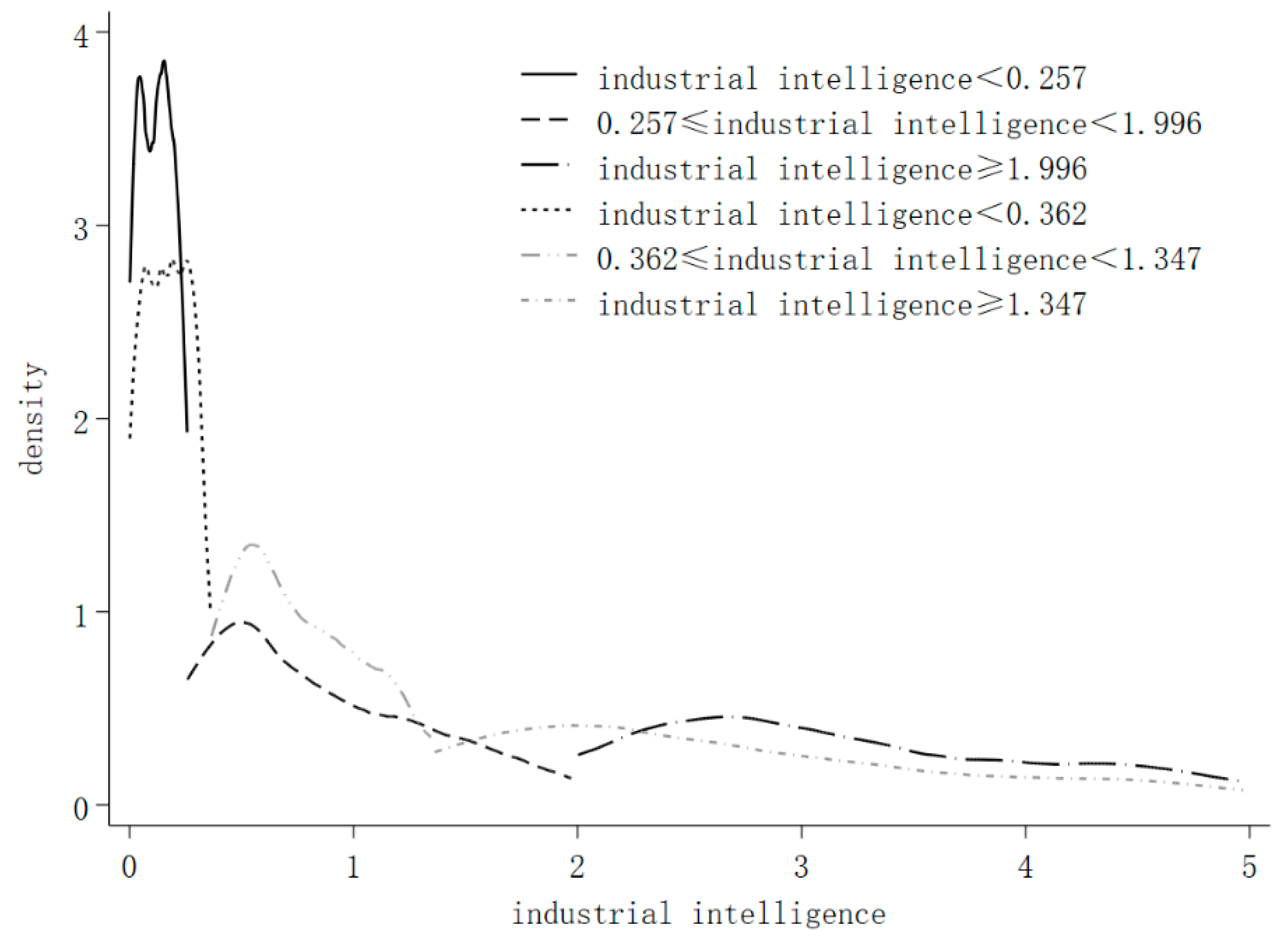
The above results indicate that as the level of industrial intelligence increases, on balance, labor cost promotes GTPF. Furthermore, this paper explores whether the impact of labor costs on GTFP is non-linear at different stages of industrial intelligence. In order to test the existence of this characteristic, the sample is divided into ‘low-level’, ‘middle-level’ and ‘high-level’ groups according to quantile values of industrial intelligence for grouped regression estimation in this paper. To test the robustness of the results, two grouping criteria are used: 25% quantile and 75% quantile as well as 33% quantile and 66% quantile. The former corresponds to the intervals [0.002, 0.257], [0.257, 1.996] and [1.996, 36.161], and the latter corresponds to the intervals [0.002, 0.362], [0.362, 1.347] and [1.347, 36.161]. Figure 1 shows the kernel density in different intervals of industrial intelligence. It can be seen that the shape of the kernel density among the intervals gradually flattens and the peak is increasingly not concentrated in a small area as the level of industrial intelligence rises. This indicates that the higher the level of industrial intelligence, the greater the gap between the provinces’ industrial intelligence development. Some provinces have a high level of industrial intelligence development, while some provinces have a very low level.

Table 5. Grouped estimation results.

Variables	(1)	(2)	(3)	(4)	(5)	(6)
$\ln lc$	−0.348	0.075 ***	1.423 ***	0.106 *	0.005	0.770 ***
	(0.269)	(0.014)	(0.289)	(0.055)	(0.042)	(0.137)
$\ln open$	−0.026	−0.003	0.324 ***	−0.063 ***	−0.071 ***	0.103
	(0.065)	(0.007)	(0.062)	(0.023)	(0.010)	(0.064)
$\ln rd$	−1.484	−0.007	−0.169	−0.090 *	0.088 ***	0.233 **
	(1.280)	(0.022)	(0.285)	(0.047)	(0.014)	(0.100)
$\ln er$	0.016	−0.015 ***	−0.054	−0.001	0.001	−0.105 ***
	(0.021)	(0.004)	(0.040)	(0.008)	(0.005)	(0.031)
$\ln urb$	0.915	−0.008	1.660	0.196	0.101 *	−0.231
	(0.622)	(0.050)	(1.369)	(0.210)	(0.053)	(0.846)
$\ln edu$	−0.131	−0.064	1.337 **	0.163	−0.028	0.375 ***
	(0.176)	(0.039)	(0.571)	(0.129)	(0.022)	(0.139)
$\ln gov$	0.633	−0.033	−0.065	−0.278 ***	−0.013	−0.106
	(0.741)	(0.028)	(0.162)	(0.048)	(0.036)	(0.068)
$\ln st$	−1.299	0.037	−1.417 ***	−0.044	0.236 ***	−0.026
	(1.463)	(0.047)	(0.459)	(0.101)	(0.046)	(0.273)
$L.gtfp$	−0.709	1.376 ***	0.619 ***	0.675 ***	1.032 ***	0.737 ***
	(0.986)	(0.059)	(0.201)	(0.090)	(0.115)	(0.063)
$constant$	−2.744	−1.065 ***	−12.375 ***	−1.302 **	0.418	−5.798 ***
	(4.967)	(0.184)	(2.857)	(0.546)	(0.311)	(1.045)
$\mathrm{N}$	54	141	75	73	95	102
$Sargan test$	1.000	0.999	1.000	1.000	0.999	1.000
$\mathrm{AR}\left(2\right)$	0.347	0.752	0.665	0.584	0.194	0.494

Note: * p < 0.1, ** p < 0.05, *** p < 0.01, standard errors are in parentheses.

reports the estimation results based on the above six intervals with the two-step system GMM method. Columns (1), (2) and (3) correspond to ‘low-level’, ‘middle-level’ and ‘high-level’ intervals of the first classification, respectively, and columns (4), (5) and (6) have a similar correspondence. In terms of coefficients direction, all coefficients of labor costs are positive except for column (1), which is consistent with the previous results. In terms of coefficient significance, the coefficients of labor cost in columns (1) and (5) are insignificant, while the coefficients are significantly positive at the 1% confidence level at the high development level stage, which again indirectly verifies the causal effect of labor costs on GTFP. In terms of coefficient size, overall, the coefficients keep getting larger as the stage of industrial intelligence development increases. The coefficients are the largest at the high development stage with 1.423 and 0.770, respectively, which are much larger than the marginal effect derived from the moderating effect. This indicates that the promotion effect of rising labor cost on GTFP is based on the development of industrial intelligence.

5.4. Threshold Model Regression Results

For the moderating effect, the non-linear effect using the squared term test has the disadvantage of left-right symmetry of the inflection point. For grouped regression estimation, the grouping criteria has the disadvantage of being subjective. Therefore, this section will empirically analyze the threshold characteristics according to model (3) by taking the industrial intelligence as the threshold variable and the labor costs as the regime-dependent variable. We use the bootstrap method to test whether the threshold effect is significant, and the number of threshold effects. The number of bootstraps is designed to be 300 times, and the number of grid points is 400.

The estimation results are shown in

Table 6. Threshold effect test and threshold results.

Dependent Variable	Type	Threshold Value	F Value	p Value	95% Confidence Intervals	BS Number
GTFP	Single Threshold	1.416	61.16 **	0.013	[1.380, 1.459]	300
	Double Threshold	1.494	86.37 **	0.013	[1.476, 1.513]	300
	Triple Threshold	2.018	48.84 ***	0.010	[2.001, 2.072]	300
GTE	Single Threshold	1.061	7.64	0.657	[1.060, 1.147]	300
	Double Threshold	1.197	0.21	1.000	[1.065, 1.202]	300
	Triple Threshold	1.494	5.02	0.627	[1.476, 1.513]	300
GTP	Single Threshold	0.267	93.76 ***	0.000	[0.154, 0.271]	300
	Double Threshold	1.575	38.16 **	0.033	[1.454, 1.577]	300
	Triple Threshold	2.001	27.81	0.350	[1.202, 2.018]	300

Note: ** p < 0.05, *** p < 0.01

. With GTFP as the dependent variable, industrial intelligence passed the testing of single threshold, double threshold, and triple threshold at 5%, 5%, and 1% confidence levels, respectively, indicating that there is a triple threshold. Three thresholds’ values (1.416, 1.494 and 2.018; 4.121, 4.455, and 7.523, respectively, after exponentiation) describe the non-linear relationship between labor costs and GTFP. These three thresholds divide the industrial intelligence into four intervals. Similarly, the p values are all more than 10% with GTE as the dependent variable, which means that there is no threshold effect. With GTP as the dependent variable, industrial intelligence passes the double threshold testing at a 5% confidence level, while the p value is more than 10% in the triple threshold testing, suggesting that a double threshold model is appropriate for the analysis. Two thresholds’ values (0.267; 1.575), which divide the industrial intelligence into three intervals, are described the non-linear relationship.

The threshold regression results are listed in

Table 7. Threshold model results.

Dependent Variable	Threshold Interval	Coefficient	Standard Error	p Value	95% Confidence Interval
GTFP	$\ln ii$ ≤ 1.416	0.453 ***	0.120	0.000	[0.216, 0.690]
	$1.416 < \ln ii$ ≤ 1.494	0.855 ***	0.128	0.000	[0.602, 1.108]
	$1.494 < \ln ii$ ≤ 2.018	0.479 ***	0.120	0.000	[0.243, 0.714]
	$\ln ii$ > 2.018	0.559 ***	0.121	0.000	[0.321, 0.797]
GTP	$\ln ii$ ≤ 0.267	0.452 ***	0.082	0.000	[0.291, 0.614]
	$0.267 < \ln ii$ ≤ 1.575	0.477 ***	0.081	0.000	[0.318, 0.636]
	$\ln ii$ > 1.575	0.530 ***	0.080	0.000	[0.371, 0.699]

Note: *** p < 0.01, control variables are controlled.

. Firstly, we test the non-linear effect of labor costs on GTFP. When $\ln ii$ is below 1.416, the coefficient of labor costs is 0.453; when $\ln ii$ is between 1.416 and 1.494, the coefficient is 0.855, showing a relatively large increase; when $\ln ii$ further rises to 2.018, the coefficient decreases to 0.479, but it is still greater than the lowest interval coefficient; when $\ln ii$ is greater than 2.018, the coefficient continues to rise to 0.559. The first threshold value of 1.416 corresponds to about an 88% quantile of industrial intelligence, indicating that the degree of industrial intelligence in most provinces is now still below the minimum threshold value. It is more right-skewed compared to the 66% quantile and 75% quantile in the previous grouped regressions. In 2019, there were 14 provinces with industrial intelligence greater than the first threshold, 11 provinces greater than the second threshold, and 6 provinces greater than the third threshold, namely Fujian, Guangdong, Zhejiang, Henan, Jiangsu and Shandong. There is a sudden increase in the coefficient in the second interval. The possible reason is that during this period, labor and the new generation of digital technologies are able to produce better complementary effects. In other words, the high-skilled and high-productivity human capital screened by the rising labor cost is matched with the new technology at this time. On balance, the labor costs coefficient still tends to rise, so the promotion effect of rising labor costs on GTFP is increasing with the deepening of industrial intelligence. It supports Hypothesis 3.

Secondly, we test the non-linear effect of labor costs on GTP. When industrial intelligence is below the threshold value of 0.267, the coefficient is 0.452; when the threshold interval rises between 0.267 and 1.575, the coefficient rises to 0.477, and when it crosses the threshold value of 1.575, the coefficient continues to rise to 0.530. All the above coefficients pass the 1% significance test. Therefore, this implies that there is also a progressively increasing positive moderating effect of industrial intelligence. The first threshold corresponds to about 64% of the quantile, implying that industrial intelligence plays a moderating role between labor costs and GTP earlier than GTFP.

5.5. Robustness Test

To enhance the robustness of the results, robustness tests are conducted in three ways. Firstly, drawing on the study of Chen et al. [26], this paper employs the directional distance function (DDF) and the Global Malmquist–Luenberger (GML) productivity index to re-measure GTFP (GTFP1) with the same input-output variables as above. Secondly, we use social insurance premiums ($lc1$) replacing wages to measure labor costs. Specifically, we select four employee insurance programs: medical insurance, pension insurance, work injury insurance and unemployment insurance, then add up the four per-capita social security fund incomes to represent social insurance premiums. Based on the above two variables, we re-estimate the models (1) and (2) using a two-step systematic GMM method. The estimation results are shown in column (1) to column (4) of Table 4. Thirdly, we change the estimation method. This paper uses a panel Tobit model for estimation, given that GTFP measured by SBM-GML has non-negative truncation characteristics and is a restricted dependent variable. Column (5) and (6) show the results. Comparing

Table 8. Robustness test results.

Variables	(1)	(2)	(3)	(4)	(5)	(6)
	Replacing GTFP		Replacing Labor Costs		Panel Tobit Estimates
$\ln lc$	0.040 ***	0.089 ***			0.615 ***	0.406 ***
	(0.008)	(0.013)			(0.105)	(0.142)
$\ln lc1$			0.096 ***	0.212 ***
			(0.021)	(0.049)
$\ln ii$		−0.219 ***		−0.141 ***		−2.216 ***
		(0.033)		(0.021)		(0.314)
$\ln lc\times \ln ii$		0.027 ***				0.290 ***
		(0.004)				(0.038)
$\ln lc1\times \ln ii$				0.056 ***
				(0.009)
$\ln open$	0.015 ***	0.017 **	0.012	−0.124 ***	−0.012	0.070
	(0.005)	(0.008)	(0.017)	(0.037)	(0.064)	(0.055)
$\ln rd$	0.003	0.003	0.089 ***	0.262 ***	0.290 ***	0.142
	(0.005)	(0.010)	(0.028)	(0.093)	(0.109)	(0.093)
$\ln er$	−0.013 ***	−0.009 ***	−0.064 ***	−0.022 **	−0.075 **	−0.016
	(0.001)	(0.002)	(0.010)	(0.011)	(0.037)	(0.033)
$\ln urb$	0.082 ***	−0.019	0.079	−0.164	−0.431	−0.196
	(0.020)	(0.035)	(0.119)	(0.257)	(0.303)	(0.252)
$\ln edu$	0.029 **	−0.004	0.128 **	−0.044	0.055	0.115
	(0.012)	(0.015)	(0.061)	(0.077)	(0.214)	(0.185)
$\ln gov$	0.021 **	−0.000	0.089	−0.149	−0.236 *	−0.018
	(0.009)	(0.013)	(0.057)	(0.093)	(0.128)	(0.116)
$\ln st$	−0.025 **	−0.007	−0.191 ***	0.089	0.470 ***	0.141
	(0.010)	(0.034)	(0.061)	(0.194)	(0.181)	(0.137)
$constant$	−0.323 ***	−0.581 ***	−0.220	0.249	−3.228 ***	−1.560
	(0.056)	(0.131)	(0.175)	(0.473)	(1.173)	(1.392)
N	270	270	270	270	300	300
$Sargan test$	0.999	1.000	1.000	1.000
$AR(2)$	0.250	0.340	0.420	0.190

Note: * p < 0.1, ** p < 0.05, *** p < 0.01, standard errors are in parentheses.

with Table 3 and Table 4, we find that the empirical results are consistent with those reported previously, proving that the results we achieved are robust.

6. Conclusions and Policy Recommendations

Based on a panel of 30 Chinese provinces from 2010 to 2019, this paper investigates the relationship between labor costs, industrial intelligence and GTFP by a two-step system GMM estimation model, moderating effect model and threshold regression models. The empirical results show that the rise of labor costs plays a significant promotional role in China’s GTFP. Moreover, rising labor costs have a dampening effect on GTE while promoting GTP; an increase in labor costs by 1% could increase GTP by about 0.499% while decreasing GTE by about 0.107%. This indicates that the mechanism of labor costs promoting GTFP is mainly to enhance GTP. The results also reveal that industrial intelligence has a positive moderating effect and can significantly strengthen the contribution of labor costs to GTFP and GTP while having a “U-shaped” moderating effect on GTE. Moreover, the boosting effect of labor costs is greater and more significant only when industrial intelligence is developed to a higher level. Furthermore, on balance, there is a significant enhanced positive non-linear characteristic between labor costs and GTFP with industrial intelligence as the threshold variable. At present, the level of industrial intelligence development in most provinces is below the first threshold value, indicating that the industrial intelligence base for green development brought about by rising labor costs still has great potential for development.

There are two viewpoints in the existing research: Firstly, the capital-substituted labor caused by rising labor costs has firm heterogeneity. The coping strategy of small and financially constrained firms is to reduce labor input. Secondly, it is difficult for companies with strong financing constraints to absorb high labor costs through technological innovation and thereby increase the TFP. Our conclusions are consistent with these views. It is relatively difficult for enterprises with small scales and strong financing constraints to quickly realize intelligent production. Then, the positive moderating effect of industrial intelligence on the innovation effect and the factor substitution effect will become very weak. The contribution of labor costs to GTFP will then be largely limited. On the contrary, large-scale enterprises with strong financing capabilities are more likely to realize intelligent production, and the effect of factor structure will be exerted to promote the continuous growth of GTFP, instead of facing rising labor costs in vain.

To better enable China’s rising labor costs to become more of a driving force for green transformation, this paper proposes the following countermeasures: (1) Active attention is paid to identifying the sources of rising labor cost factors. There are many reasons for the rise of labor costs, and the most consistent with the market law is that the increase of labor productivity drives up the price of labor factors. We should pay attention to the passive increase in labor costs caused by the aging population, the expansion of university enrollment and the “devaluation of education” and mitigate the labor market confusion caused by these factors. In addition, we should improve the matching of high human capital with high wage levels in order to maximize the innovation and complementary effects when labor costs rise. (2) Accelerating the process of industrial intelligence. In the face of the disappearance of the demographic dividend and the challenge of “de-industrialization”, we should seize the opportunity to develop a new generation of information and digital technology to force the innovation of manufacturing production technology, process organization re-engineering and value-chain upgrading. (3) Reasonably promoting the protection and transformation of innovation achievements. The promotion from technological innovation to green low-carbon production needs to go through a series of processes. On the one hand, legislative protection and R&D subsidies should be strengthened to give enterprises the social benefits of overflowing innovation results. On the other hand, we should give full play to the important role of industrial Internet platforms in interconnection, resource sharing and complementary collaboration.

References

1. Lee, S.; Oh, D.W. Economic growth and the environment in China: Empirical evidence using prefecture level data. China Econ. Rev. 2015, 36, 73–85. [Google Scholar] [CrossRef]
2. Huang, H.Y.; Mo, R.B.; Chen, X.Q. New patterns in China’s regional green development: An interval Malmquist–Luenberger productivity analysis. Struct. Change Econ. Dyn. 2021, 58, 161–173. [Google Scholar] [CrossRef]
3. Cai, F. The second demographic dividend as a driver of China’s growth. China World Econ. 2020, 28, 26–44. [Google Scholar] [CrossRef]
4. Li, H.B.; Li, L.; Wu, B.Z.; Xiong, Y.Y. The end of cheap Chinese labor. J. Econ. Perspect. 2012, 26, 57–74. [Google Scholar] [CrossRef]
5. Chen, F.W.; Tan, Y.L.; Chen, F.Z.; Wu, Y.Q. Enhancing or suppressing: The effect of labor costs on energy intensity in emerging economies. Energy 2021, 214, 118964. [Google Scholar] [CrossRef]
6. Zhang, Q.A.; Zhang, F.F.; Mai, Q. Robot adoption and green productivity: Curse or Boon. Sustain. Prod. Consum. 2022, 34, 1–11. [Google Scholar] [CrossRef]
7. Du, P.C.; Xu, S. Minimum wages, market evolution and productivity growth. Ind. Econ. Res. 2020, 90–101. (In Chinese) [Google Scholar] [CrossRef]
8. Mayneris, F.; Poncet, S.; Zhang, T. Improving or disappearing: Firm-level adjustments to minimum wages in China. J. Dev. Econ. 2018, 135, 20–42. [Google Scholar] [CrossRef] [Green Version]
9. Yang, L.G.; Liu, J.F.; Han, F. Research on the influence of minimum wage standard on green total factor productivity. Theory Pract. Financ. Econ. 2022, 43, 128–134. (In Chinese) [Google Scholar] [CrossRef]
10. Fan, H.C.; Hu, Y.C.; Tang, L.X. Labor costs and the adoption of robots in China. J. Econ. Behav. Organ. 2021, 186, 608–631. [Google Scholar] [CrossRef]
11. Li, Y.Y.; Zhang, Y.R.; Pan, A.; Han, M.C.; Veglianti, E. Carbon emission reduction effects of industrial robot applications: Heterogeneity characteristics and influencing mechanisms. Technol. Soc. 2022, 70, 102034. [Google Scholar] [CrossRef]
12. Zhao, P.Y.; Gao, Y.; Sun, X. How does artificial intelligence affect green economic growth?—Evidence from China. Sci. Total Environ. 2022, 834, 155306. [Google Scholar] [CrossRef] [PubMed]
13. Tang, J.; Feng, J. Do social security contributions affect the capital-labor ratio: Evidence from China. Econ. Res. J. 2019, 54, 87–101. (In Chinese) [Google Scholar]
14. Tan, C.X.; Lin, X.L. Research on the impact of social insurance pressure on enterprise total factor productivity: Evidence from the implementation of the “Social Insurance Law” in 2011. Mod. Ind. Econ. 2022, 15, 137–151. (In Chinese) [Google Scholar] [CrossRef]
15. Wei, T.Y.; Zhu, Q.; Glomsrød, S. A general equilibrium view of population ageing impact on energy use via labor supply. Sustainability 2017, 9, 1534. [Google Scholar] [CrossRef] [Green Version]
16. Hu, R.D.; Cao, J.B. The impact of population aging on total factor productivity of China’s manufacturing enterprises: Based on the empirical analysis of Shanghai and Shenzhen A-share listed manufacturing companies. West Forum 2021, 31, 100–111. (In Chinese) [Google Scholar] [CrossRef]
17. Acemoglu, D.; Restrepo, P. Demographics and automation. Rev. Econ. Stud. 2022, 89, 1–44. [Google Scholar] [CrossRef]
18. Xian, J.K.; Wang, W.; Lan, S. Would population aging cause capital to replace labor? South China J. Econ. 2022, 41, 43–62. (In Chinese) [Google Scholar] [CrossRef]
19. Liu, Y.Y.; Liu, B. Employment protection legislation, cost stickiness, and corporate response. Econ. Res. J. 2014, 49, 63–76. (In Chinese) [Google Scholar]
20. Xiao, W.; Xue, T.H. Rising labor costs, financial constraints and changing TFP of enterprises in China. China Ocean. J. World Econ. 2019, 42, 76–94. (In Chinese) [Google Scholar]
21. Zhang, Y.J.; Song, Y.; Zou, H. Transformation of pollution control and green development: Evidence from China’s chemical industry. J. Environ. Manag. 2020, 275, 111246. [Google Scholar] [CrossRef] [PubMed]
22. Mao, J.H.; Wu, Q.; Zhu, M.H.; Lu, C.P. Effects of environmental regulation on green total factor productivity: An Evidence from the yellow river basin, China. Sustainability 2022, 14, 2015. [Google Scholar] [CrossRef]
23. Li, D.; Hu, S.M. How does technological innovation mediate the relationship between environmental regulation and high-quality economic development? Empirical evidence from China. Sustainability 2021, 13, 2231. [Google Scholar] [CrossRef]
24. Song, M.L.; Peng, L.C.; Shang, Y.P.; Zhao, X. Green technology progress and total factor productivity of resource-based enterprises: A perspective of technical compensation of environmental regulation. Technol. Forecast. Soc. Change 2022, 174, 121276. [Google Scholar] [CrossRef]
25. Yuan, B.L.; Ren, S.G.; Chen, X.H. Can environmental regulation promote the coordinated development of economy and environment in China’s manufacturing industry?—A panel data analysis of 28 sub-sectors. J. Clean. Prod. 2017, 149, 11–24. [Google Scholar] [CrossRef]
26. Chen, C.F.; Lan, Q.X.; Gao, M.; Sun, Y.W. Green total factor productivity growth and its determinants in China’s industrial economy. Sustainability 2018, 10, 1052. [Google Scholar] [CrossRef] [Green Version]
27. He, L.Y.; Qi, X.F. Environmental regulation and green total factor productivity: Evidence from Chinese Industrial Enterprises. Econ. Perspect. 2022, 6, 97–114. (In Chinese) [Google Scholar]
28. Yuan, J.Q.; Zhang, D.Y. Research on the impact of environmental regulations on industrial green total factor productivity: Perspectives on the changes in the allocation ratio of factors among different industries. Sustainability 2021, 13, 12947. [Google Scholar] [CrossRef]
29. Cai, W.G.; Zhou, X.L. Dual effect of Chinese environmental regulation on green total factor productivity. Economist 2017, 27–35. (In Chinese) [Google Scholar] [CrossRef]
30. Wu, L.; Jia, X.Y.; Wu, C.; Peng, J.C. Impact of heterogeneous environmental regulation on green total factors productivity. China Popul. Resour. Environ. 2020, 30, 82–92. (In Chinese) [Google Scholar] [CrossRef]
31. Qiu, S.L.; Wang, Z.L.; Geng, S.S. How do environmental regulation and foreign investment behavior affect green productivity growth in the industrial sector? An empirical test based on Chinese provincial panel data. J. Environ. Manag. 2021, 287, 112282. [Google Scholar] [CrossRef] [PubMed]
32. Lin, B.Q.; Chen, Z.Y. Does factor market distortion inhibit the green total factor productivity in China? J. Clean. Prod. 2018, 197, 25–33. [Google Scholar] [CrossRef]
33. Bian, Y.C.; Wu, L.H.; Bai, J.H.; Yang, Y.Z. Does factor market distortion restrain the green economic growth? World Econ. Pap. 2021, 105–119. (In Chinese) [Google Scholar]
34. Zhao, N.; Li, X.J.; Li, G.Q. Fiscal vertical imbalance, factor price distortion and green TFP: Evidence from 266 China’s cities. Theory Pract. Financ. Econ. 2021, 42, 91–100. (In Chinese) [Google Scholar] [CrossRef]
35. Deng, C.X.; Zhao, H.; Xie, B.G.; Li, Z.W.; Li, K. The impacts of land misallocation on urban industrial green total-factor productivity in China. Acta Geogr. Sin. 2021, 76, 1865–1881. (In Chinese) [Google Scholar] [CrossRef]
36. Zhang, D.Y. Marketization, environmental regulation, and eco-friendly productivity: A Malmquist–Luenberger index for pollution emissions of large Chinese firms. J. Asian Econ. 2021, 76, 101342. [Google Scholar] [CrossRef]
37. Draca, M.; Machin, S.; Van Reenen, J. Minimum wages and firm profitability. Am. Econ. J. Appl. Econ. 2011, 3, 129–151. [Google Scholar] [CrossRef] [Green Version]
38. Motta, V. Lack of access to external finance and SME labor productivity: Does project quality matter? Small Bus. Econ. 2020, 54, 119–134. [Google Scholar] [CrossRef]
39. Bai, X.J.; Yu, Q.R. How does labor costs affect China’s industrialization? Financ. Trade Econ. 2019, 40, 132–145. (In Chinese) [Google Scholar] [CrossRef]
40. Xie, M.M.; Ding, L.; Xia, Y.; Guo, J.F.; Pan, J.F.; Wang, H.J. Does artificial intelligence affect the pattern of skill demand? Evidence from Chinese manufacturing firms. Econ. Model. 2021, 96, 295–309. [Google Scholar] [CrossRef]
41. Vermeulen, B.; Pyka, A.; Saviotti, P.P. Robots, structural change, and employment: Future scenarios. In Handbook of Labor, Human Resources and Population Economics; Zimmermann, K.F., Ed.; Springer International Publishing: Cham, Switzerland, 2020; pp. 1–37. [Google Scholar] [CrossRef]
42. Acemoglu, D.; Restrepo, P. Automation and new tasks: How technology displaces and reinstates labor. J. Econ. Perspect. 2019, 33, 3–30. [Google Scholar] [CrossRef] [Green Version]
43. Acemoglu, D.; Restrepo, P. Robots and jobs: Evidence from US labor markets. J. Political Econ. 2020, 128, 2188–2244. [Google Scholar] [CrossRef] [Green Version]
44. Wang, Y.F.; Xie, L.; Zhang, Y.; Wang, C.Y.; Yu, K. Does FDI promote or inhibit the high-quality development of agriculture in China? An agricultural GTFP perspective. Sustainability 2019, 11, 4620. [Google Scholar] [CrossRef] [Green Version]
45. Arellano, M.; Bond, S. Some tests of specification for panel data: Monte Carlo evidence and an application to employment equations. Rev. Econ. Stud. 1991, 58, 277–297. [Google Scholar] [CrossRef]
46. Arellano, M.; Bover, O. Another look at the instrumental variable estimation of error-components models. J. Econom. 1995, 68, 29–51. [Google Scholar] [CrossRef] [Green Version]
47. Blundell, R.; Bond, S. Initial conditions and moment restrictions in dynamic panel data models. J. Econom. 1998, 87, 115–143. [Google Scholar] [CrossRef] [Green Version]
48. Jiang, T. Mediating effects and moderating effects in causal inference. China Ind. Econ. 2022, 100–120. (In Chinese) [Google Scholar] [CrossRef]
49. Hansen, B.E. Threshold effects in non-dynamic panels: Estimation, testing, and inference. J. Econom. 1999, 93, 345–368. [Google Scholar] [CrossRef] [Green Version]
50. Liu, Z.K.; Xin, L. Has China’s Belt and Road Initiative promoted its green total factor productivity? Evidence from primary provinces along the route. Energy Policy 2019, 129, 360–369. [Google Scholar] [CrossRef]
51. Fang, L.; Hu, R.; Mao, H.; Chen, S.J. How crop insurance influences agricultural green total factor productivity: Evidence from Chinese farmers. J. Clean. Prod. 2021, 321, 128977. [Google Scholar] [CrossRef]
52. Tone, K. A slacks-based measure of efficiency in data envelopment analysis. Eur. J. Oper. Res. 2001, 130, 498–509. [Google Scholar] [CrossRef] [Green Version]
53. Oh, D.H. A global Malmquist-Luenberger productivity index. J. Product. Anal. 2010, 34, 183–197. [Google Scholar] [CrossRef]
54. Yang, D.T.; Chen, V.W.; Monarch, R. Rising wages: Has China lost its global labor advantage? Pac. Econ. Rev. 2010, 15, 482–504. [Google Scholar] [CrossRef] [Green Version]
55. Fan, H.C.; Lin, F.Q.; Tang, L.X. Minimum wage and outward FDI from China. J. Dev. Econ. 2018, 135, 1–19. [Google Scholar] [CrossRef]
56. Ren, S.G.; Yuan, B.L.; Ma, X.; Chen, X.H. International trade, FDI (foreign direct investment) and embodied CO2 emissions: A case study of Chinas industrial sectors. China Econ. Rev. 2014, 28, 123–134. [Google Scholar] [CrossRef]
57. Liu, S.M.; Hou, P.; Gao, Y.K.; Tan, Y. Innovation and green total factor productivity in China: A linear and nonlinear investigation. Environ. Sci. Pollut. Res. 2022, 29, 12810–12831. [Google Scholar] [CrossRef]
58. Gollin, D.; Jedwab, R.; Vollrath, D. Urbanization with and without industrialization. J. Econ. Growth 2016, 21, 35–70. [Google Scholar] [CrossRef]
59. Sadorsky, P. Do urbanization and industrialization affect energy intensity in developing countries? Energy Econ. 2013, 37, 52–59. [Google Scholar] [CrossRef]
60. Wang, M.; Xu, M.; Ma, S.J. The effect of the spatial heterogeneity of human capital structure on regional green total factor productivity. Struct. Change Econ. Dyn. 2021, 59, 427–441. [Google Scholar] [CrossRef]
61. Zhao, J.; Jiang, Q.Z.; Dong, X.C.; Dong, K.Y.; Jiang, H.D. How does industrial structure adjustment reduce CO2 emissions? Spatial and mediation effects analysis for China. Energy Econ. 2022, 105, 105704. [Google Scholar] [CrossRef]
Figure 1. Industrial intelligence interval kernel density. Note: The figure shows the original value of industrial intelligence after indexing l n i i ; to show the density more clearly, the right end of industrial intelligence is intercepted to 5, which does not affect the basic conclusion as there are only 26 samples greater than 5, and adding them would only increase the flatness of the high development level stage.
Sustainability 14 13653 g001