

Characterizing the Long-Term Landscape Dynamics of a Typical Cloudy Mountainous Area in Northwest Yunnan, China

Abstract
:1. Introduction
- (1)
- To propose a composite approach to address large volumes of cloud-cover satellite imagery and map high time–frequency LTS in mountainous areas.
- (2)
- To characterize and estimate landscape dynamics using the LTS maps in the EHW.
2. Materials and Methods
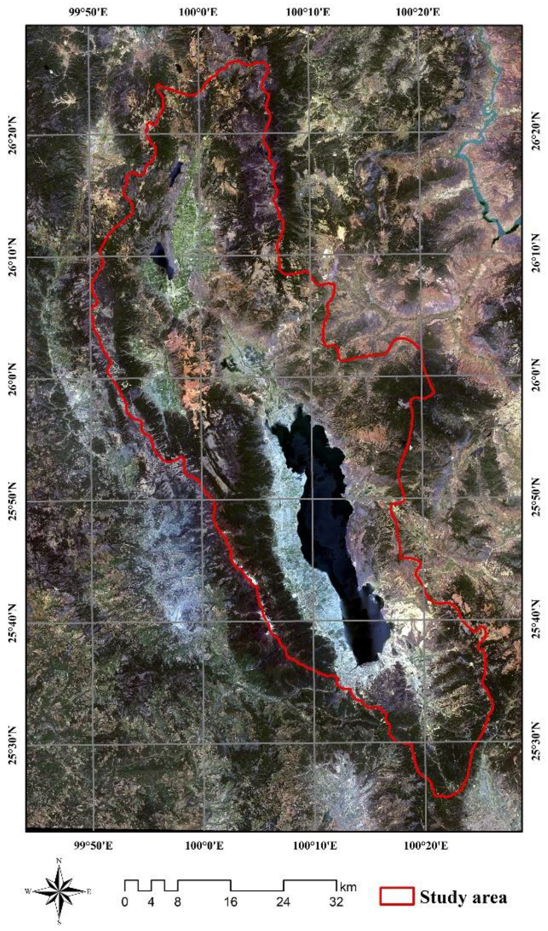
2.1. Study Area
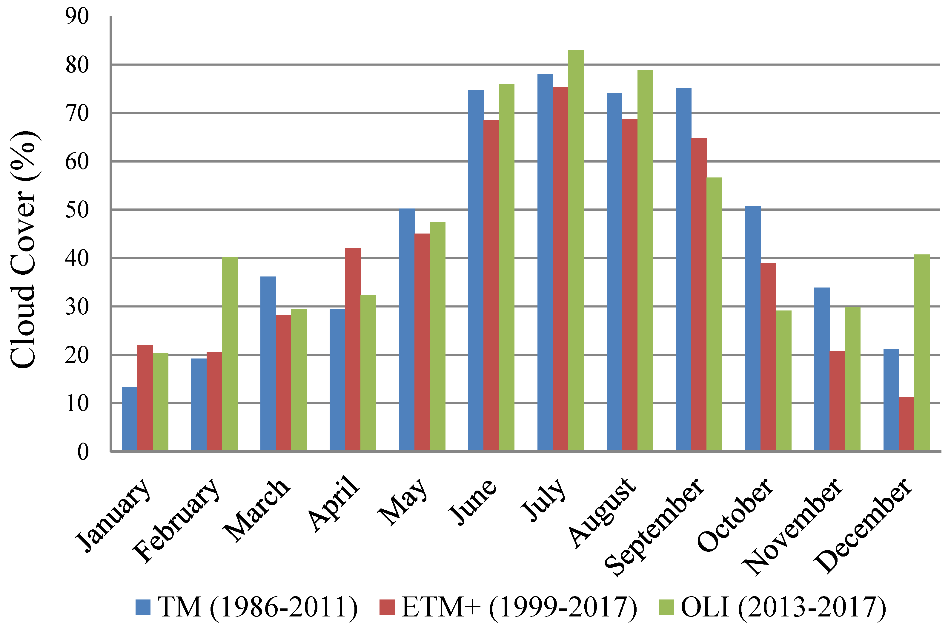
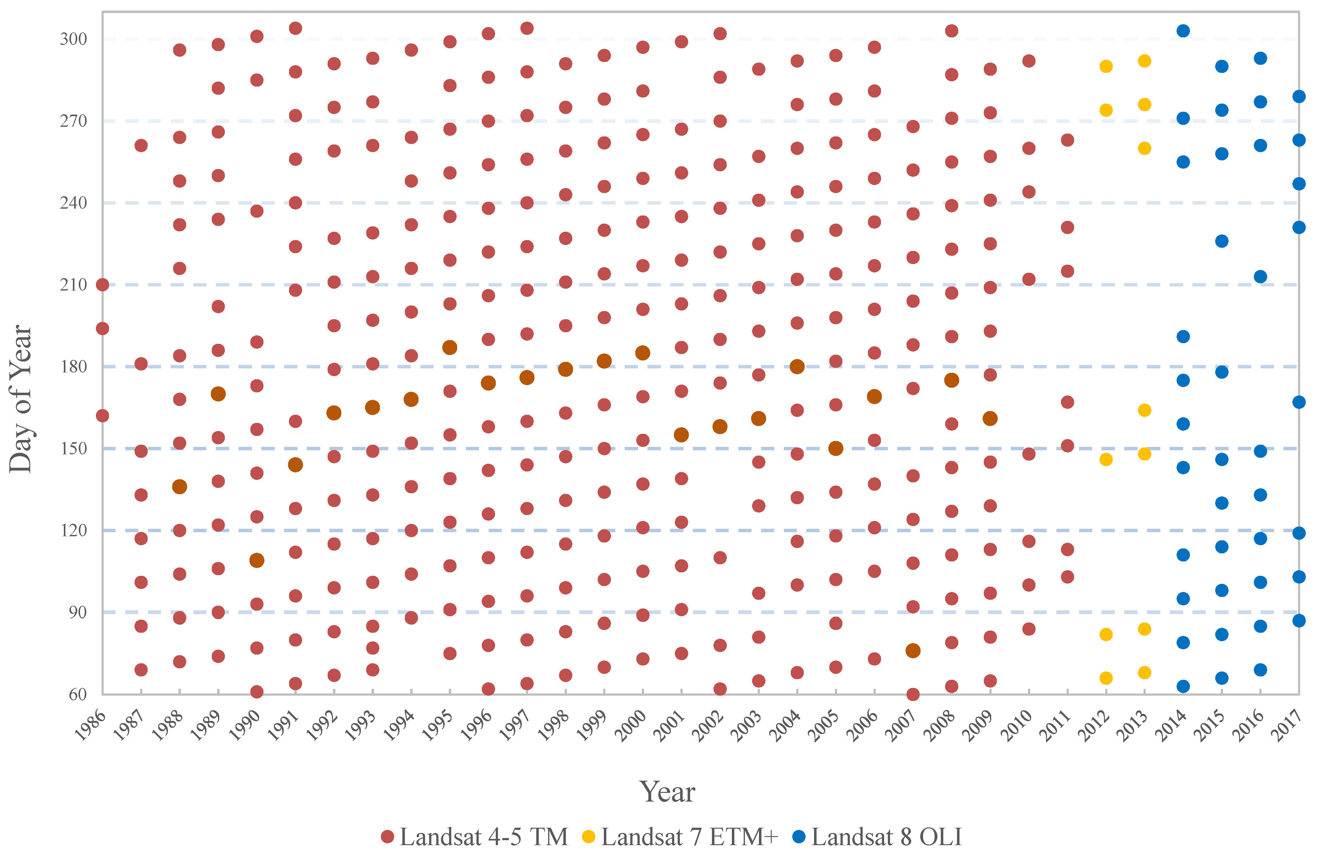
2.2. Data Used
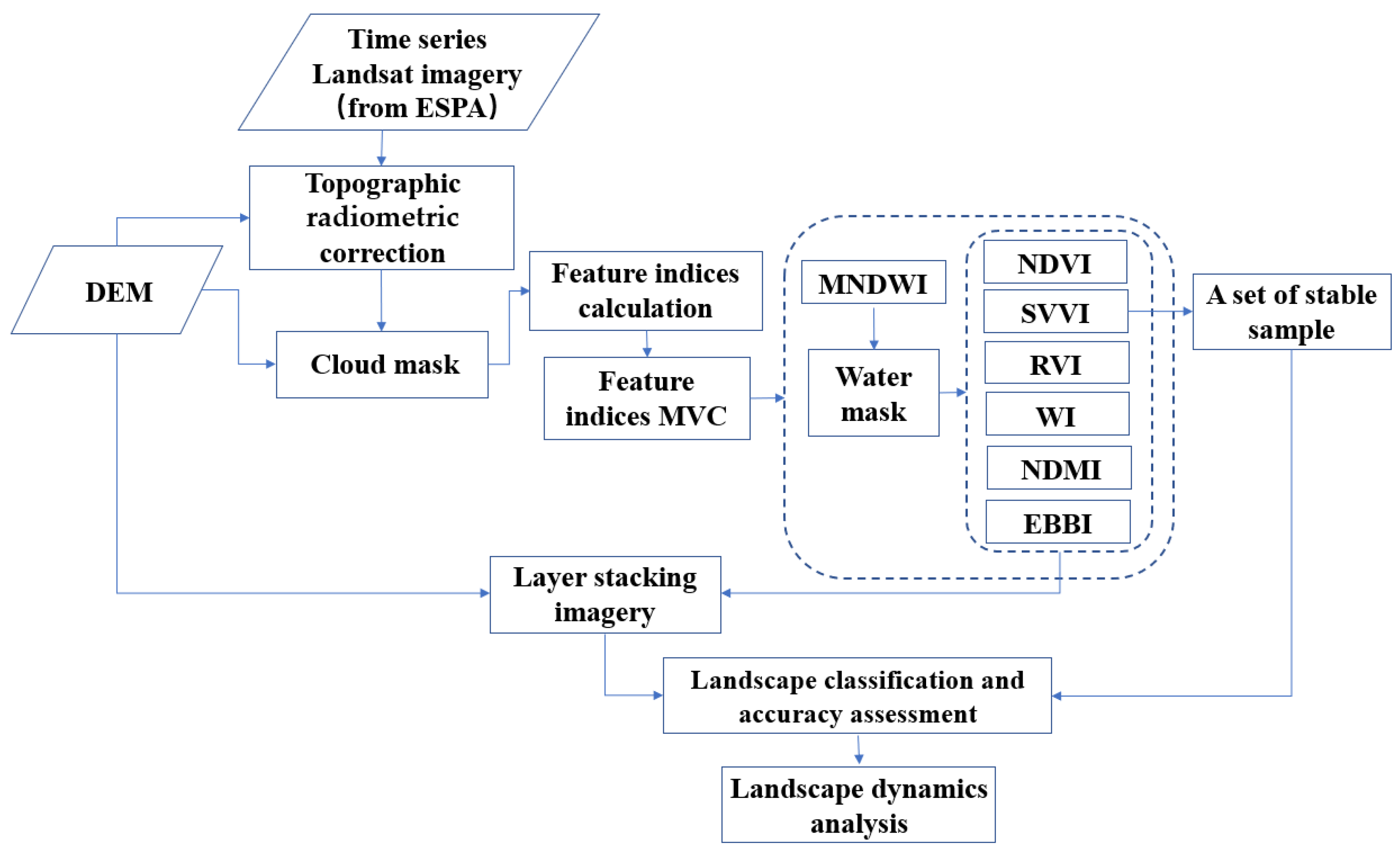
2.3. Methods
2.3.1. Topographic Radiometric Correction
2.3.2. Cloud Mask
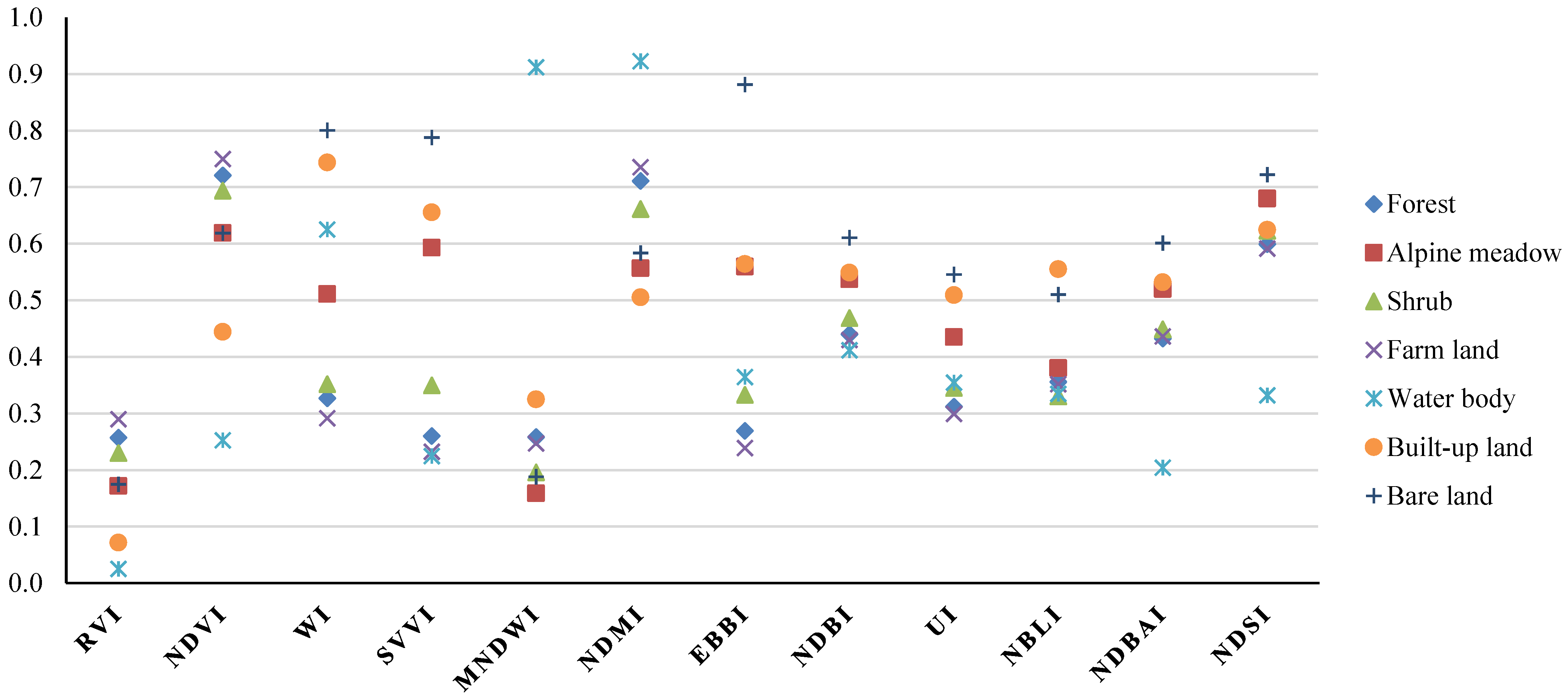
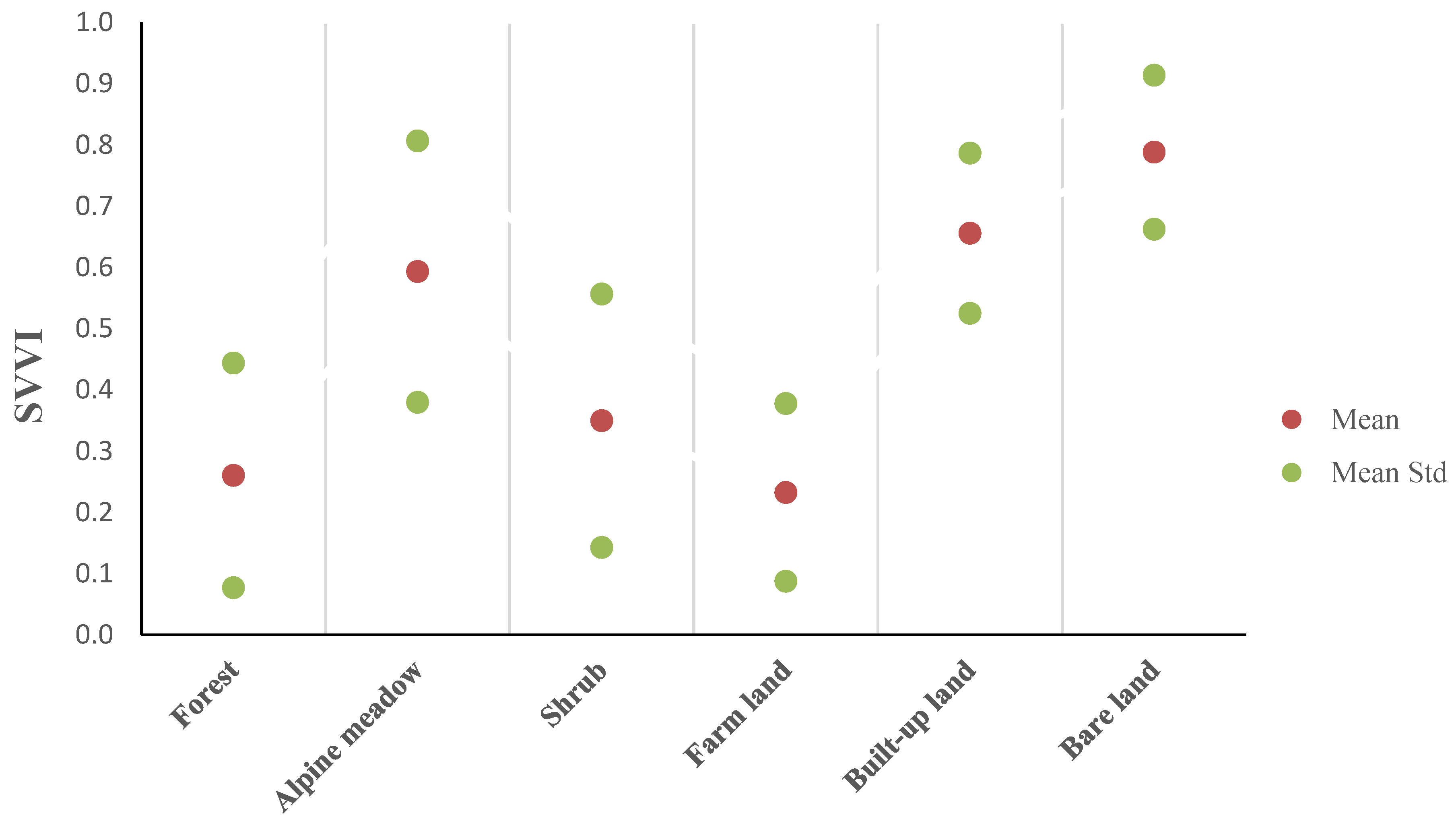
2.3.3. Feature Index Derivation and Image Composition
2.3.4. Masking Out of Water Bodies and Selection of Stable Samples
2.3.5. Landscape Classification and Landscape Dynamics Analysis
- (1)
- Landscape classification and accuracy assessment
- (2)
- Analysis of landscape dynamics
3. Results
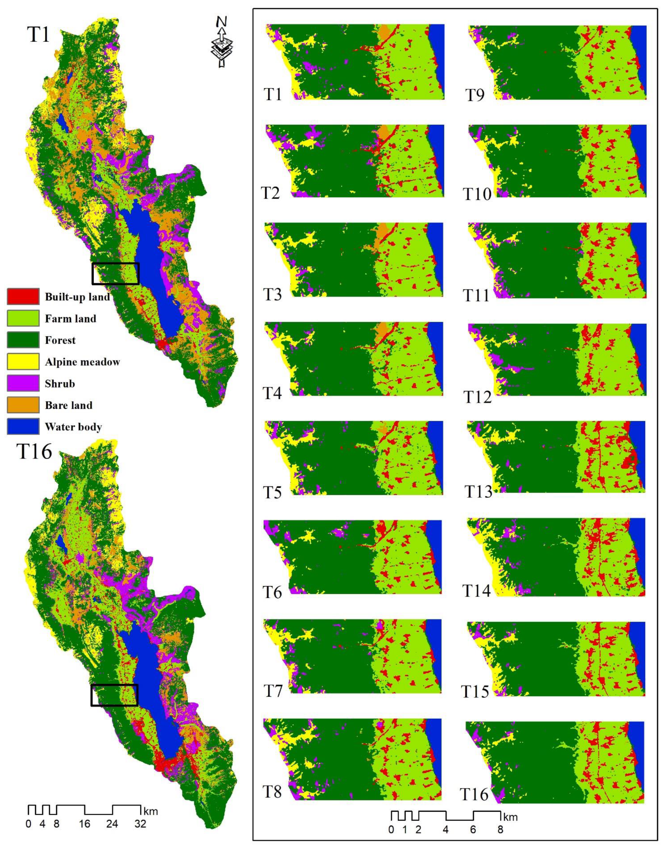
3.1. Landscape Classification
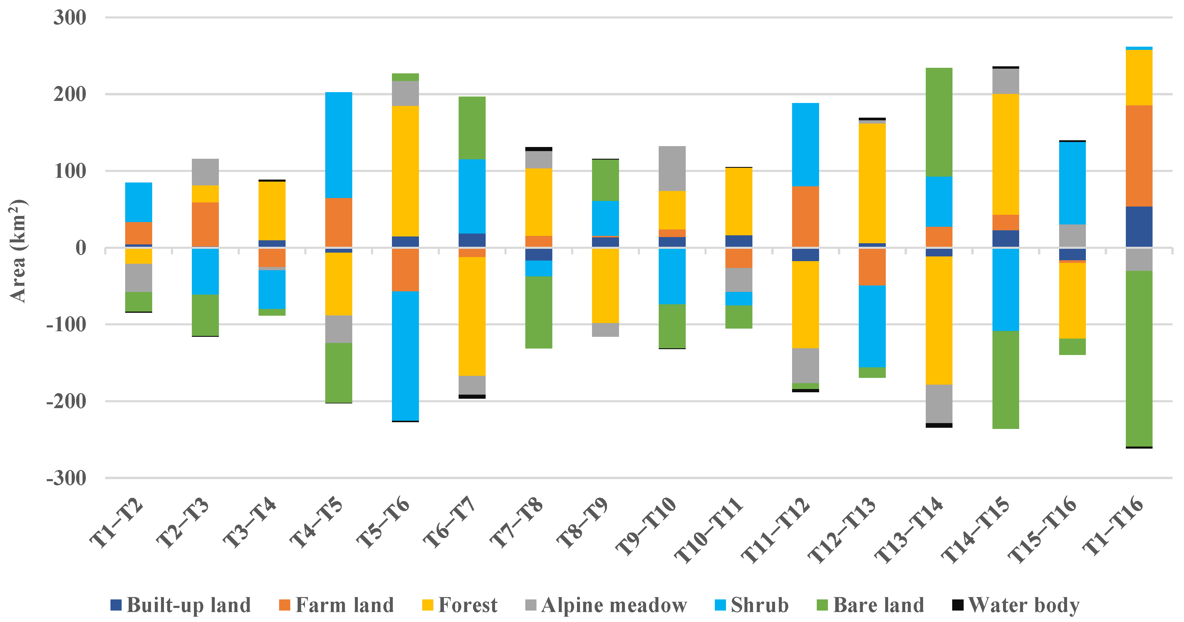
3.2. Changes in Landscape Composition
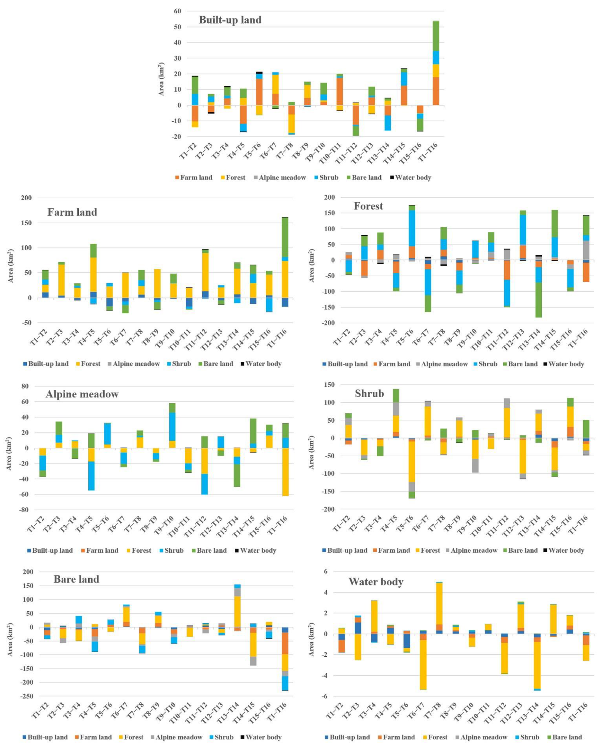
3.3. Landscape Transformation
3.4. Changes in Landscape Pattern Indices
4. Discussion
5. Conclusions
Author Contributions
Funding
Data Availability Statement
Acknowledgments
Conflicts of Interest
References
- Wang, Y.; Xia, T.; Shataer, R.; Zhang, S.; Li, Z. Analysis of Characteristics and Driving Factors of Land-Use Changes in the Tarim River Basin from 1990 to 2018. Sustainability 2021, 13, 10263. [Google Scholar] [CrossRef]
- Parihar, S.M.; Pandey, V.K.; Anshu; Shree, K.; Moin, K.; Ali, M.B.; Narasimhan, K.; Rai, J.; Kamil, A. Land Use Dynamics and Impact on Regional Climate Post-Tehri Dam in the Bhilangana Basin, Garhwal Himalaya. Sustainability 2022, 14, 10221. [Google Scholar] [CrossRef]
- Yang, L.; Wang, Z.; Jin, G.; Chen, D.; Wang, Z. Geological risk assessment for the rapid development area of the Erhai Basin. Phys. Chem. Earth Parts A/B/C 2015, 89–90, 79–90. [Google Scholar] [CrossRef]
- Peng, J.; Ma, J.; Du, Y.; Zhang, L.; Hu, X. Ecological suitability evaluation for mountainous area development based on conceptual model of landscape structure, function, and dynamics. Ecol. Indic. 2016, 61, 500–511. [Google Scholar] [CrossRef]
- Peng, J.; Du, Y.; Liu, Y.; Hu, X. How to assess urban development potential in mountain areas? An approach of ecological carrying capacity in the view of coupled human and natural systems. Ecol. Indic. 2016, 60, 1017–1030. [Google Scholar] [CrossRef]
- Xu, J.; Wilkes, A. Biodiversity impact analysis in northwest Yunnan, southwest China. Biodivers. Conserv. 2004, 13, 959–983. [Google Scholar] [CrossRef]
- Zhang, Y.; Wang, T.; Cai, C.; Li, C.; Liu, Y.; Bao, Y.; Guan, W. Landscape pattern and transition under natural and anthropogenic disturbance in an arid region of northwestern China. Int. J. Appl. Earth Obs. Geoinf. 2016, 44, 1–10. [Google Scholar] [CrossRef]
- Sulla-Menashe, D.; Friedl, M.A.; Woodcock, C.E. Sources of bias and variability in long-term Landsat time series over Canadian boreal forests. Remote Sens. Environ. 2016, 177, 206–219. [Google Scholar] [CrossRef]
- Li, X.; Gong, P.; Liang, L. A 30-year (1984–2013) record of annual urban dynamics of Beijing City derived from Landsat data. Remote Sens. Environ. 2015, 166, 78–90. [Google Scholar] [CrossRef]
- Nyland, K.E.; Gunn, G.E.; Shiklomanov, N.I.; Engstrom, R.N.; Streletskiy, D.A. Land Cover Change in the Lower Yenisei River Using Dense Stacking of Landsat Imagery in Google Earth Engine. Remote Sens. 2018, 10, 1226. [Google Scholar] [CrossRef]
- Vuolo, F.; Ng, W.-T.; Atzberger, C. Smoothing and gap-filling of high resolution multi-spectral time series: Example of Landsat data. Int. J. Appl. Earth Obs. Geoinf. 2017, 57, 202–213. [Google Scholar] [CrossRef]
- Zhang, L.; Weng, Q. Annual dynamics of impervious surface in the Pearl River Delta, China, from 1988 to 2013, using time series Landsat imagery. ISPRS J. Photogramm. Remote Sens. 2016, 113, 86–96. [Google Scholar] [CrossRef]
- Moreira, E.P.; Valeriano, M.M. Application and evaluation of topographic correction methods to improve land cover mapping using object-based classification. Int. J. Appl. Earth Obs. Geoinf. 2014, 32, 208–217. [Google Scholar] [CrossRef]
- Li, H.; Wang, C.; Zhong, C.; Zhang, Z.; Liu, Q. Mapping Typical Urban LULC from Landsat Imagery without Training Samples or Self-Defined Parameters. Remote Sens. 2017, 9, 700. [Google Scholar] [CrossRef] [Green Version]
- Griffiths, P.; van der Linden, S.; Kuemmerle, T.; Hostert, P. A Pixel-Based Landsat Compositing Algorithm for Large Area Land Cover Mapping. IEEE J. Sel. Top. Appl. Earth Obs. Remote Sens. 2013, 6, 2088–2101. [Google Scholar] [CrossRef]
- Hermosilla, T.; Wulder, M.A.; White, J.C.; Coops, N.C.; Hobart, G.W. An integrated Landsat time series protocol for change detection and generation of annual gap-free surface reflectance composites. Remote Sens. Environ. 2015, 158, 220–234. [Google Scholar] [CrossRef]
- Xu, L.; Li, B.; Yuan, Y.; Gao, X.; Zhang, T. A Temporal-Spatial Iteration Method to Reconstruct NDVI Time Series Datasets. Remote Sens. 2015, 7, 8906–8924. [Google Scholar] [CrossRef] [Green Version]
- Malambo, L.; Heatwole, C.D. A Multitemporal Profile-Based Interpolation Method for Gap Filling Nonstationary Data. IEEE Trans. Geosci. Remote Sens. 2016, 54, 252–261. [Google Scholar] [CrossRef]
- Eivazi, A.; Kolesnikov, A.; Junttila, V.; Kauranne, T. Variance-preserving mosaicing of multiple satellite images for forest parameter estimation: Radiometric normalization. ISPRS J. Photogramm. Remote Sens. 2015, 105, 120–127. [Google Scholar] [CrossRef]
- Jiang, Z.-G.; Brosse, S.; Jiang, X.-M.; Zhang, E. Measuring ecosystem degradation through half a century of fish species introductions and extirpations in a large isolated lake. Ecol. Indic. 2015, 58, 104–112. [Google Scholar] [CrossRef]
- Wang, X.; Yu, S.; Huang, G.H. Land allocation based on integrated GIS-optimization modeling at a watershed level. Landsc. Urban Plan. 2004, 66, 61–74. [Google Scholar] [CrossRef]
- Guo, H.C.; Liu, L.; Huang, G.H.; Fuller, G.A.; Zou, R.; Yin, Y.Y. A system dynamics approach for regional environmental planning and management: A study for the Lake Erhai Basin. J. Environ. Manag. 2001, 61, 93–111. [Google Scholar] [CrossRef] [PubMed] [Green Version]
- Griffiths, P.; Kuemmerle, T.; Baumann, M.; Radeloff, V.C.; Abrudan, I.V.; Lieskovsky, J.; Munteanu, C.; Ostapowicz, K.; Hostert, P. Forest disturbances, forest recovery, and changes in forest types across the Carpathian ecoregion from 1985 to 2010 based on Landsat image composites. Remote Sens. Environ. 2014, 151, 72–88. [Google Scholar] [CrossRef]
- Nitze, I.; Grosse, G. Detection of landscape dynamics in the Arctic Lena Delta with temporally dense Landsat time-series stacks. Remote Sens. Environ. 2016, 181, 27–41. [Google Scholar] [CrossRef]
- Soenen, S.A.; Peddle, D.R.; Coburn, C.A. SCS+C: A modified Sun-canopy-sensor topographic correction in forested terrain. IEEE Trans. Geosci. Remote Sens. 2005, 43, 2148–2159. [Google Scholar] [CrossRef]
- Qiu, S.; He, B.; Zhu, Z.; Liao, Z.; Quan, X. Improving Fmask cloud and cloud shadow detection in mountainous area for Landsats 4–8 images. Remote Sens. Environ. 2017, 199, 107–119. [Google Scholar] [CrossRef]
- Person, R. Remote mapping of standing crop biomass for estimation of the productivity of the short-grass Prairie. In Proceedings of the Eighth International Symposium on Remote Sensing of Environment, Ann Arbor, MI, USA, 2–6 October 1972; Willow Run Laboratories: Brighton, MI, USA, 1972. [Google Scholar]
- Tucker, C.J. Red and photographic infrared linear combinations for monitoring vegetation. Remote Sens. Environ. 1979, 8, 127–150. [Google Scholar] [CrossRef] [Green Version]
- Lehmann, E.A.; Wallace, J.F.; Caccetta, P.A.; Furby, S.L.; Zdunic, K. Forest cover trends from time series Landsat data for the Australian continent. Int. J. Appl. Earth Obs. Geoinf. 2013, 21, 453–462. [Google Scholar] [CrossRef]
- Coulter, L.L.; Stow, D.A.; Tsai, Y.-H.; Ibanez, N.; Shih, H.-C.; Kerr, A.; Benza, M.; Weeks, J.R.; Mensah, F. Classification and assessment of land cover and land use change in southern Ghana using dense stacks of Landsat 7 ETM+ imagery. Remote Sens. Environ. 2016, 184, 396–409. [Google Scholar] [CrossRef]
- Xu, H. Modification of normalised difference water index (NDWI) to enhance open water features in remotely sensed imagery. Int. J. Remote Sens. 2007, 27, 3025–3033. [Google Scholar] [CrossRef]
- Wilson, E.H.; Sader, S.A. Detection of forest harvest type using multiple dates of Landsat TM imagery. Remote Sens. Environ. 2002, 80, 385–396. [Google Scholar] [CrossRef]
- As-syakur, A.R.; Adnyana, I.W.S.; Arthana, I.W.; Nuarsa, I.W. Enhanced Built-Up and Bareness Index (EBBI) for Mapping Built-Up and Bare Land in an Urban Area. Remote Sens. 2012, 4, 2957–2970. [Google Scholar] [CrossRef] [Green Version]
- Zha, Y.; Gao, J.; Ni, S. Use of normalized difference built-up index in automatically mapping urban areas from TM imagery. Int. J. Remote Sens. 2010, 24, 583–594. [Google Scholar] [CrossRef]
- Hongmei, Z.; Xiaoling, C. Use of normalized difference bareness index in quickly mapping bare areas from TM/ETM+. In Proceedings of the International Geoscience and Remote Sensing Symposium, Seoul, Korea, 25–29 July 2005; IEEE: New York, NY, USA, 2005. [Google Scholar]
- Li, H.; Wang, C.; Zhong, C.; Su, A.; Xiong, C.; Wang, J.; Liu, J. Mapping Urban Bare Land Automatically from Landsat Imagery with a Simple Index. Remote Sens. 2017, 9, 249. [Google Scholar] [CrossRef] [Green Version]
- Rogers, A.S.; Kearney, M.S. Reducing signature variability in unmixing coastal marsh Thematic Mapper scenes using spectral indices. Int. J. Remote Sens. 2010, 25, 2317–2335. [Google Scholar] [CrossRef]
- Zheng, B.; Myint, S.W.; Thenkabail, P.S.; Aggarwal, R.M. A support vector machine to identify irrigated crop types using time-series Landsat NDVI data. Int. J. Appl. Earth Obs. Geoinf. 2015, 34, 103–112. [Google Scholar] [CrossRef]
- Puyravaud, J.-P. Standardizing the calculation of the annual rate of deforestation. For. Ecol. Manag. 2003, 177, 593–596. [Google Scholar] [CrossRef]
- Walz, U. Indicators to monitor the structural diversity of landscapes. Ecol. Model. 2015, 295, 88–106. [Google Scholar] [CrossRef]
- McGarigal, K.; Marks, B.J. FRAGSTATS: Spatial Pattern Analysis Program for Quantifying Landscape Structure; U.S. Department of Agriculture, Forest Service, Pacific Northwest Research Station: Portland, OR, USA, 1995.
- Cao, X.; Liu, Y.; Liu, Q.; Cui, X.; Chen, X.; Chen, J. Estimating the age and population structure of encroaching shrubs in arid/semiarid grasslands using high spatial resolution remote sensing imagery. Remote Sens. Environ. 2018, 216, 572–585. [Google Scholar] [CrossRef]
- Zhao, Y.; Feng, D.; Yu, L.; Cheng, Y.; Zhang, M.; Liu, X.; Xu, Y.; Fang, L.; Zhu, Z.; Gong, P. Long-Term Land Cover Dynamics (1986–2016) of Northeast China Derived from a Multi-Temporal Landsat Archive. Remote Sens. 2019, 11, 599. [Google Scholar] [CrossRef]
- Stenzel, S.; Feilhauer, H.; Mack, B.; Metz, A.; Schmidtlein, S. Remote sensing of scattered Natura 2000 habitats using a one-class classifier. Int. J. Appl. Earth Obs. Geoinf. 2014, 33, 211–217. [Google Scholar] [CrossRef]
- Németh, G.; Lóczy, D.; Gyenizse, P. Long-Term Land Use and Landscape Pattern Changes in a Marshland of Hungary. Sustainability 2021, 13, 12664. [Google Scholar] [CrossRef]


| Name | Unit | Description |
|---|---|---|
| MPS | km2 | MPS is the average size of patch of a landscape type [41]. An increase in the MPS usually indicates a decrease in fragmentation. |
| LPI | % | LPI is a simple dominance measure, which is the percentage of the total landscape area constituting the largest patch [41]. |
| TE | km | TE is the total edge length of a particular patch type [41]. Increasing the TE typically indicates an increase in the complexity of the patch shape. |
| MENN | m | MENN distance is the average shortest straight-line distance between nearest neighbor of the same class [41]. MENN has been used extensively to quantify patch isolation. |
| Time | Overall Accuracy | Forest | Alpine Meadow | Shrub | Farmland | Built-Up Land | Bare Land | ||||||
|---|---|---|---|---|---|---|---|---|---|---|---|---|---|
| Pr | Us | Pr | Us | Pr | Us | Pr | Us | Pr | Us | Pr | Us | ||
| T1: 1986–1987 | 82.72 | 81.87 | 85.49 | 76.66 | 78.57 | 82.00 | 79.46 | 92.00 | 93.24 | 98.20 | 83.21 | 74.78 | 78.18 |
| T2: 1988–1989 | 81.99 | 83.01 | 80.13 | 78.08 | 81.43 | 76.83 | 77.13 | 95.33 | 96.62 | 97.22 | 80.15 | 70.54 | 82.73 |
| T3: 1990–1991 | 81.75 | 81.35 | 83.91 | 72.82 | 77.50 | 85.15 | 75.58 | 89.57 | 98.65 | 96.52 | 84.73 | 73.21 | 74.55 |
| T4: 1992–1993 | 82.80 | 81.82 | 82.33 | 73.38 | 76.79 | 83.75 | 77.91 | 96.67 | 97.97 | 99.19 | 93.13 | 72.27 | 78.18 |
| T5: 1994–1995 | 82.40 | 81.42 | 82.97 | 77.27 | 78.93 | 78.63 | 75.58 | 92.31 | 97.3 | 100 | 93.13 | 73.39 | 72.73 |
| T6: 1996–1997 | 83.12 | 83.97 | 82.65 | 72.35 | 80.36 | 84.28 | 74.81 | 96.05 | 98.65 | 98.39 | 93.13 | 74.14 | 78.18 |
| T7: 1998–1999 | 82.32 | 80.6 | 85.17 | 73.00 | 78.21 | 83.7 | 73.64 | 95.92 | 95.27 | 96.77 | 91.60 | 75.68 | 76.36 |
| T8: 2000–2001 | 86.17 | 84.33 | 84.86 | 80.63 | 81.79 | 81.99 | 82.95 | 96.67 | 97.97 | 99.23 | 98.47 | 86.00 | 78.18 |
| T9: 2002–2003 | 85.29 | 86.08 | 83.91 | 78.05 | 80.00 | 79.70 | 82.17 | 96.00 | 97.30 | 99.22 | 96.95 | 84.62 | 80.00 |
| T10: 2004–2005 | 84.00 | 81.87 | 85.49 | 73.67 | 73.93 | 82.79 | 78.29 | 98.64 | 97.97 | 99.23 | 98.47 | 81.98 | 82.73 |
| T11: 2006–2007 | 83.92 | 83.44 | 82.65 | 74.59 | 80.71 | 82.55 | 75.19 | 98.00 | 99.32 | 99.22 | 97.71 | 76.99 | 79.09 |
| T12: 2008–2009 | 84.08 | 87.50 | 81.70 | 78.28 | 81.07 | 78.36 | 81.40 | 89.94 | 96.62 | 95.97 | 90.84 | 82.24 | 80.00 |
| T13: 2010–2011 | 87.30 | 89.63 | 84.54 | 78.38 | 82.86 | 87.11 | 86.43 | 95.97 | 96.62 | 98.48 | 99.24 | 80.36 | 81.82 |
| T14: 2012–2013 | 85.61 | 87.5 | 83.91 | 78.69 | 81.79 | 83.97 | 85.27 | 95.3 | 95.95 | 94.62 | 93.89 | 78.70 | 77.27 |
| T15: 2014–2015 | 86.98 | 87.03 | 86.75 | 77.74 | 83.57 | 88.46 | 80.23 | 97.33 | 98.65 | 99.23 | 98.47 | 80.53 | 82.73 |
| T16: 2016–2017 | 88.18 | 85.85 | 88.01 | 80.34 | 83.21 | 91.70 | 85.66 | 96.05 | 98.65 | 97.73 | 98.47 | 85.58 | 80.91 |
Publisher’s Note: MDPI stays neutral with regard to jurisdictional claims in published maps and institutional affiliations. |
© 2022 by the authors. Licensee MDPI, Basel, Switzerland. This article is an open access article distributed under the terms and conditions of the Creative Commons Attribution (CC BY) license (https://creativecommons.org/licenses/by/4.0/).
Share and Cite
Chen, Y.; Hu, X.; Zhang, Y.; Feng, J. Characterizing the Long-Term Landscape Dynamics of a Typical Cloudy Mountainous Area in Northwest Yunnan, China. Sustainability 2022, 14, 13488. https://doi.org/10.3390/su142013488
Chen Y, Hu X, Zhang Y, Feng J. Characterizing the Long-Term Landscape Dynamics of a Typical Cloudy Mountainous Area in Northwest Yunnan, China. Sustainability. 2022; 14(20):13488. https://doi.org/10.3390/su142013488
Chicago/Turabian StyleChen, Youjun, Xiaokang Hu, Yanjie Zhang, and Jianmeng Feng. 2022. "Characterizing the Long-Term Landscape Dynamics of a Typical Cloudy Mountainous Area in Northwest Yunnan, China" Sustainability 14, no. 20: 13488. https://doi.org/10.3390/su142013488