Multi-Modal Graph Interaction for Multi-Graph Convolution Network in Urban Spatiotemporal Forecasting

Abstract

Graph convolution network-based approaches have been recently used to model region-wise relationships in region-level prediction problems in urban computing. Each relationship represents a kind of spatial dependency, such as region-wise distance or functional similarity. To incorporate multiple relationships into a spatial feature extraction, we define the problem as a multi-modal machine learning problem on multi-graph convolution networks. Leveraging the advantage of multi-modal machine learning, we propose to develop modality interaction mechanisms for this problem in order to reduce the generalization error by reinforcing the learning of multi-modal coordinated representations. In this work, we propose two interaction techniques for handling features in lower layers and higher layers, respectively. In lower layers, we propose grouped GCN to combine the graph connectivity from different modalities for a more complete spatial feature extraction. In higher layers, we adapt multi-linear relationship networks to GCN by exploring the dimension transformation and freezing part of the covariance structure. The adapted approach, called multi-linear relationship GCN, learns more generalized features to overcome the train–test divergence induced by time shifting. We evaluated our model on a ride-hailing demand forecasting problem using two real-world datasets. The proposed technique outperforms state-of-the art baselines in terms of prediction accuracy, training efficiency, interpretability and model robustness.

1. Introduction

The deployment of urban sensor networks is one of the most important progresses in the urban digitization process. Recent advances in sensor technology enable the collection of a large variety of datasets. Multi-modality is one of the most significant features in the knowledge discovery process in urban computing. Data from different sources are often correlated with each other. For region-level prediction problems, such as crowd flow prediction [1,2] or taxi demand prediction [3,4,5], it has become a common practice to incorporate a large variety of auxiliary datasets, such as weather, Point of Interests (also known as POI), road network and events. In this paper, we define each auxiliary dataset as a modality and study multi-modal learning on multi-graph convolution networks (MGCN) for spatiotemporal prediction problems in urban computing. This task is challenging due to complex spatial dependencies and a temporal shifting generalization gap.

Designing a spatial feature extraction method is challenging due to complex region-wise spatial dependencies. GCN-based models [6,7] are first used for traffic prediction on road networks. Geng et al. [5] proposed Multi-GCN (MGCN) for generic spatiotemporal prediction tasks by stacking three GCNs. Each GCN encodes a unique modality (relationship) of auxiliary data (geo-distance, POI similarity and road network) as graph and extract spatial dependencies from such relationship.

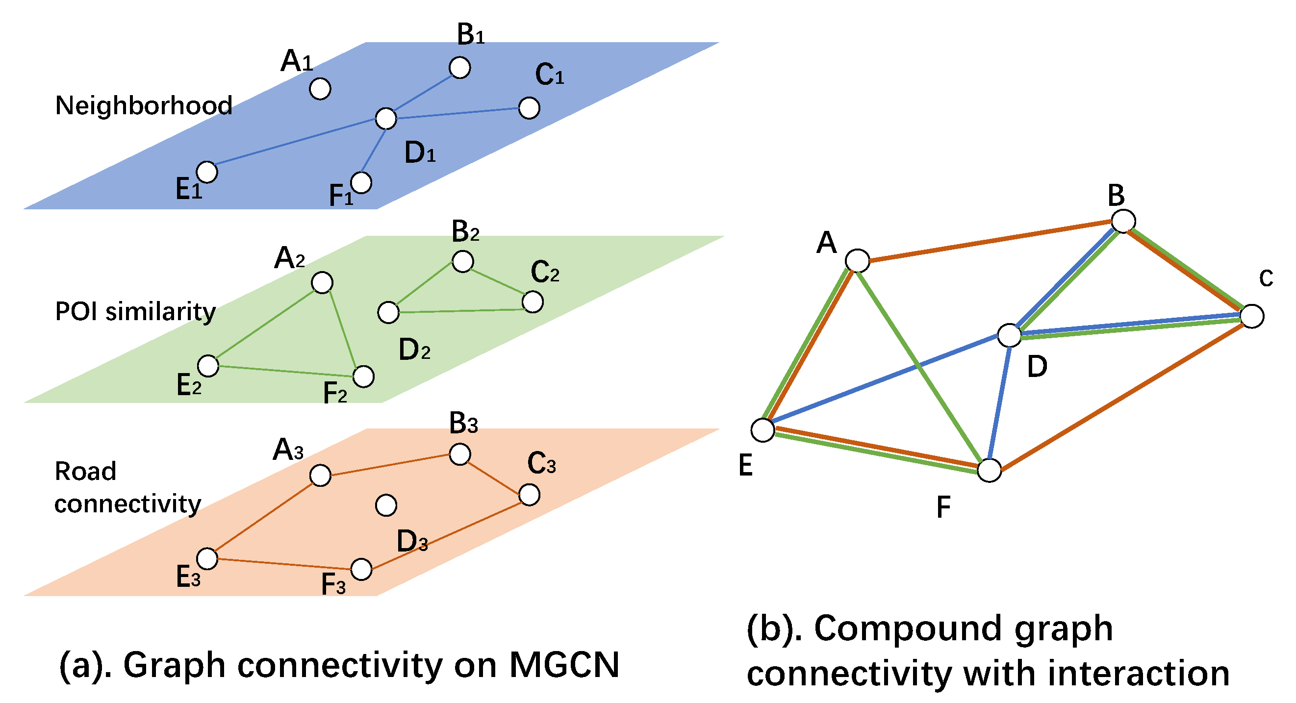
The spatial feature extraction by MGCN architecture is incomplete due to the lack of cross-graph connectivities. Figure 1 shows an example for MGCN. Consider the vertex (region) pair A and D. According to graph topology, A and D are disconnected in all three graphs. MGCN is incapable of extracting features from D for A or vice versa. However, we argue that the A-D relationship is important. The region pair $A_3$-$B_3$ and $B_2$-$D_2$ are closely related on road connectivity and POI similarity. A and D are related region pairs for spatial feature extraction. To complete the physical meaning for spatial feature extraction by MGCN, the ideal graph connectivity is shown in Figure 1b. It is produced by merging all edges from separate graphs, so that any random walk path is a compound of any kind of relationships.

Improving model generality to overcome the temporal shifting generalization gap is another challenging task. The temporal pattern for time series data varies along with time. Formally,

$$P\left(X_t\right|X_{t-1},X_{t-2},\dots )\ne P\left(X_{t^{\prime }}\right|X_{t^{\prime }-1},X_{t^{\prime }-2},\dots ),t\ne t^{\prime }$$

The gap above defines the divergence between temporal pattern distributions in two different time windows t and $t^{\prime }$. Such a time-shifting gap is often caused by time series fluctuations induced by periodicity, seasonality or miscellaneous factors such as weather variation or events. We further discovered that this gap is usually accumulative. A longer temporal interval between two timestamps causes a larger divergence between two distributions. Due to this problem, machine learning models for time series prediction tasks expire frequently. Improving model generality makes the model more robust and avoids fitting to local time series fluctuations.

We propose several graph interaction techniques to address the above problem by enhancing the learning of multi-modal coordinated representations and reinforcing the model performance. Yosinski et al. [8] studied feature transferability in deep learning. It shows that features in lower layers are more general and those in higher layers are more specific. According to this phenomenon, we designed two kinds of graph interaction mechanisms correspondingly for lower layers and higher layers.

In lower layers, input spatiotemporal signal maintains its physical properties as engineered features. According to the case in Figure 1, generating latent features via compound graph connectivity makes great sense in terms of spatial feature extraction. For lower layer spatial feature extraction, we designed grouped GCN (GGCN), which enables random walk graph convolution on compound graph connectivity. The objective of GGCN is to produce a more abstract multi-modal latent feature representation based on graph convolution operations. This technique addresses the first problem on completeness in spatial feature extraction.

Higher layer features provide high level abstractions for the input signal. It becomes meaningless to explicitly extract feature from a certain region. Leveraging some advances from multi-task learning [9], we adapt multi-linear relationship learning [10] to graph convolution networks and try to find shared information among modality-specific representations. According to characteristics in GCNs, we propose multi-linear relationship GCN (MRGCN), which imposes a tensor normal distribution as the prior distribution of multi-modality graph convolution kernels to learn an explainable, robust and fine-grained relationship among modalities. To further enhance the model generality, we propose to freeze part of the covariance structure in the covariance update algorithm in order to improve output feature independency and alleviate the feature co-adaptation problem. The proposed model generates more general high level feature abstractions. This technique also reduces model training time.

On real-world ride-hailing demand data, our model outperforms state-of-the art baselines by a significant margin. Leveraging the advantage of multi-modal and multi-task learning, our model requires less data and time to reach a low prediction error. In summary, this paper makes the following contributions:

• We propose grouped GCN to produce a compound graph connectivity on a multi-modality graph representation. It makes spatial feature extraction on GCN more complete in urban computing.
• We propose multi-linear relationship GCN to learn better coordinated representations among modalities. It improves the generality for high level abstractions.
• We conduct experiments on two large-scale real-world datasets. The proposed approach achieves more than a 10% error reduction over state-of-the-art baseline methods for ride-hailing demand forecasting.

2. Related Work

Region-level prediction in urban computing. Region-level prediction is a fundamental task in data-driven urban management. There is a rich amount of topics, including citizen flow prediction [11,12,13], traffic demand prediction [3,14,15], arrival time estimation [16] and meteorology forecasting [17,18]. For these topics, the region-wise relationships are measured as geographical distance. The spatial structures for these prediction tasks are formulated as regular graphs, which are inherently Euclidean structures. Convolution neural network-based models are used for effective prediction.

Non-Euclidean structures exist in station-based prediction tasks, including bike-flow prediction [19], traffic volume prediction [6,7,20] and point-based taxi demand prediction [4]. The spatial structures for these problems are no longer regular. Graph convolution networks are usually leveraged for spatial feature extraction in these tasks. Non-Euclidean structures also exist when incorporating auxiliary data to model region-wise relationships. Yao et al. [15] encoded a region-wise relationship as a graph and used graph embedding as external features for convolution neural networks. Geng et al. [5] used MGCN to model region-wise relationships under multiple modalities.

Multi-modality in urban computing. The core issue for multi-modal machine learning is to build models that can process or relate information from multiple modalities [21]. Traditional multi-modal machine learning problems focus on human sensory modalities, including audio–visual speech recognition [22], multi-media analysis [23] and media description [24]. In urban computing, we usually need to harness knowledge from a diverse family of related datasets. Wei et al. [25] first categorized the diversity of urban computing datasets, such as POI and air quality, as multi-modality and explored feature transferability among different modalities.

Multi-modal fusion is one of the most challenging problems in urban computing. Most existing works incorporate multi-modality auxiliary data as handcrafted features in a straightforward manner. Tong et al. [4] used multi-modality data as input features for a linear regression model. Zhang et al. [2] and Yao et al. [15] concatenated auxiliary data to high level abstractions for region-level spatiotemporal prediction networks.

GCN-based approaches encode multi-modality data as region-wise relationships and perform as a static structure in deep learning. The spatial feature extraction process on GCN is associated with these modalities. According to applications in traffic volume prediction [6] and taxi demand prediction [5], GCNs are effective in spatial feature extraction on spatial-variant modality data. However, all techniques above fail to build a relationship among modalities, which is expected to improve the generality of the learning framework.

Multi-task relationship learning. Multi-task relationship learning is a basic approach for multi-task learning. Zhang and Yeung [26] first proposed a regularized multi-task model MTRL by placing a matrix-variate normal prior on the model parameters:

$$W\sim \mathcal{M}\mathcal{N}(\mathbf{0},{\Sigma }_r,{\Sigma }_c)$$

where ${\Sigma }_r$ and ${\Sigma }_c$ are the row and column covariance. Long et al. [10] proposed Multilinear Relationship Network (MR Network), which learns the multilinear relationship on different modes for the joint-task parameter tensor as:

$$\begin{array}{c}W=[W_1;W_2;\dots ;W_t]\\ W\sim \mathcal{T}{\mathcal{N}}_{D_f\times D_c\times D_t}(\mathbf{O},{\Sigma }_f,{\Sigma }_c,{\Sigma }_t)\end{array}$$

where W refers to the joint weight by concatenating all fully connected weights from all tasks. $D_f$, $D_c$ and $D_t$ denote the feature dimension, class dimension and task dimension in the joint weight. ${\Sigma }_f$, ${\Sigma }_c$ and ${\Sigma }_t$ represent covariance for each mode. Experiment results showed that imposing a multilinear relationship regularizer on the last few fully connected layers in CNN-like structures increased the feature generality and transferability in task-specific layers.

However, MR Networks only learn multilinear relationships on fully connected layers. Other deep learning structures, such as CNN or GCN, have more complicated physical meanings.

3. Methodology

$\mathbb{A}=\{A_0,A_1,\dots ,A_{\left|M\right|}\}$ denotes adjacency matrices for different graphs. Each graph corresponds to one of the $\left|M\right|$ modalities. In the ride-hailing demand prediction problem, each graph represents a kind of pair-wise spatial relationship for regions, including neighborhood (geo-distance) $A_N$, POI similarity $A_S$ and road connectivity $A_C$ [5].

$$\begin{array}{cc}\hfill A_{N,i,j}=& \left\{\begin{array}{c}1,\mathrm{if}\mathrm{region}i\mathrm{and}j\mathrm{are}\mathrm{adjacent}\hfill \\ 0,\mathrm{otherwise}\hfill \end{array}\right.\hfill \\ \hfill A_{S,i,j}=& \mathrm{sim}(P_{v_i},P_{v_j})\hfill \\ \hfill A_{C,i,j}=& \max (0,\mathrm{conn}(v_i,v_j)-A_{N,i,j})\hfill \end{array}$$

$A_N$ defines the adjacency relationship between regions. We construct $A_N$ by connecting a vertex to its 8 neighbors in a $3\times 3$ grid. $A_S$ is the cosine similarity between POI vectors of two regions. Each entry in the POI vector represents the number of POIs in a specific category. $A_C$ indicates the connectivity between two regions. Two regions are connected as long as there is a highway or subway that directly connects them.

We define the one-step spatiotemporal prediction task for a certain modality (graph $A_i$) on a spatiotemporal observation x as:

$$\begin{array}{c}\hfill x_t=G(x_{t-1},x_{t-2},\dots ,x_{t-k};A_i)\end{array}$$

(1)

where G represents any random walk-based graph convolution network. $x_t\in {\mathbb{R}}^{\left|V\right|}$ is the temporal slice of a spatiotemporal observation at time t.

When the graph convolution operation $G:({\mathbb{R}}^{\left|V\right|\times f_1};{\mathbb{R}}^{\left|V\right|\times \left|V\right|})\to {\mathbb{R}}^{\left|V\right|\times f_2}$ is defined as the polynomial of the graph laplacian (in this work, we use a symmetric normalized laplacian: $L=I-D^{-\frac{1}{2}}A{D}^{-\frac{1}{2}}$) L with degree up to K:

$$\begin{array}{c}\hfill G_W(X;A)=\sum _{\alpha =0}^K{L}^{\alpha }X{W}_{\alpha }\end{array}$$

(2)

the above definition refers to the graph convolution operation of ChebNet [27]. In this work, we use this variation of graph convolution operations.

In the multi-modality formulation of this problem, each modality refers to a representation learning process of the same spatiotemporal observation on different graphs. Following the convention in [21], we formally joined a representation of a multi-modality learning problem on a multi-graph convolution network as:

$$\begin{array}{c}\hfill x_t={\mathcal{F}}_{A_i\in \mathbb{A}}\left(G_W(x_{t-1},x_{t-2},\dots ,x_{t-k};A_i)\right)\end{array}$$

(3)

where ${\mathcal{F}}_{A\in \mathbb{A}}$ denotes the interaction function across multi-graphs. In previous work [5], it is defined as a stacking function in anterior layers and sum function in the output layer. The major contribution of this work focuses on the design of this interaction function.

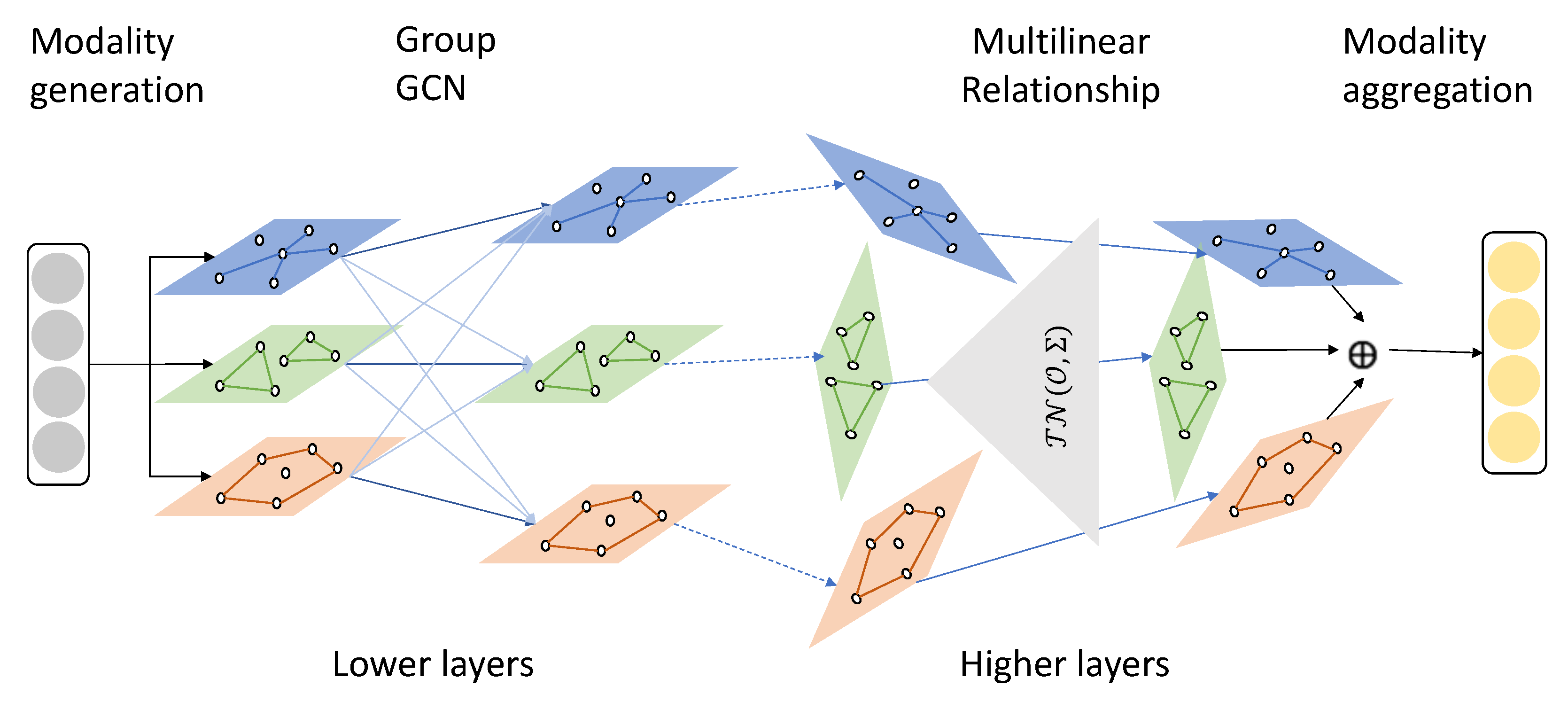
Figure 2 shows the proposed framework. According to an analysis on feature generality [8] for deep neural networks, we proposed two techniques for building modality-wise interactions targeted for lower layers and higher layers, respectively, in stacked MGCNs. In lower layers, the hidden features are concrete. The feature extraction in lower layers is usually general. Considering these facts, we propose to build inter-modality connections to enable inter-graph spatial feature extraction. To distinguish feature extraction parameters, we penalize inter-graph weight and intra-graph weight differently by group regularization. In higher layers, the hidden features are highly abstract that they can no longer maintain their physical properties. Applying inter-modality connections is not applicable. High level features are usually task specific, which is harmful to model generality and transferability. In these layers, we propose to learn a multilinear relationship on training parameters of joint modalities in order to improve the model generality and avoid overfitting the model to local fluctuations.

3.1. Grouped GCN

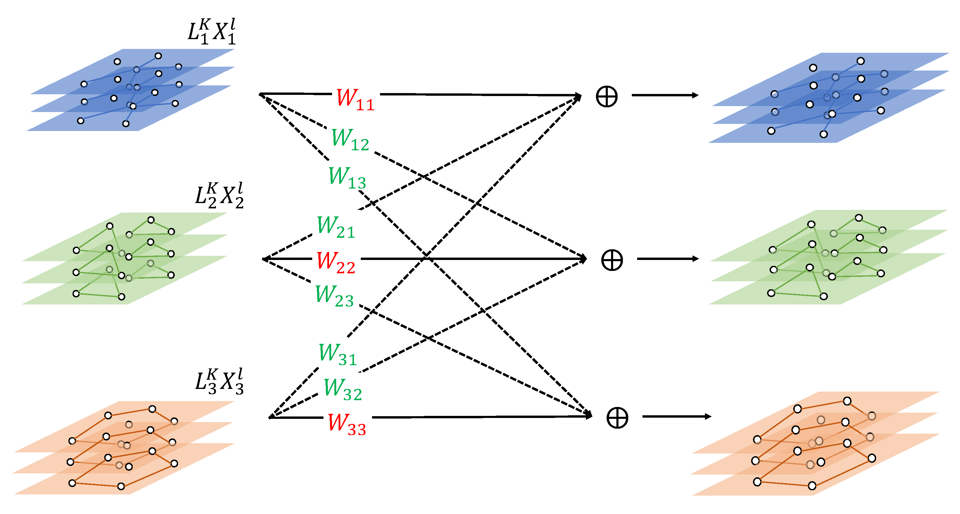
Figure 3 shows one layer transformation of grouped GCN (GGCN). In lower layers, we use GGCN to build compound graph connectivity, which enables cross-graph spatial feature extraction.

$L_i\in {\mathbb{R}}^{\left|V\right|\times \left|V\right|}$ denotes the graph laplacian matrix of the i-th modality. $X_i^l\in {\mathbb{R}}^{\left|V\right|\times f_l}$ denotes the input signal of the ith modality of the lth layer ($l,i\in {\mathbb{Z}}^{+}$). When $l=1$, $X_i^1$ represents the raw input and $X_i^1=X_j^1,\forall i,j$, we define the lth layer parameter $W^l$ as:

$$\begin{array}{c}\hfill W^l=\left(\begin{array}{cccc}{w}_{1,1}^l& w_{1,2}^l& \dots & w_{1,\left|M\right|}^l\\ w_{2,1}^l& w_{2,2}^l& \dots & w_{2,\left|M\right|}^l\\ \dots & \dots & \dots & \dots \\ w_{\left|M\right|,1}^l& w_{\left|M\right|,2}^l& \dots & w_{\left|M\right|,\left|M\right|}^l\end{array}\right),\end{array}$$

(4)

$w_{i,j}^l\in {\mathbb{R}}^{f_l\times f_{l+1}\times K}$ denotes the weight matrix to transform the ith modality input to the jth modality output via ChebNet transformation $G_{w_{i,j}^l}(X_i^l;A_i)$, where $f_l$ and $f_{l+1}$ are the feature dimension of the lth and $(l+1)$th layer. K represents the degree of the Chebyshev polynomial, which is sliced during the computation of ChebNet.

The jth modality output is computed as:

$$X_j^{l+1}=\sigma (\sum _{i=1}^{\left|M\right|}{G}_{w_{i,j}^l}(X_i^l;A_i)+b_j^l)$$

(5)

We denote all weights that transform an input to output within sthe ame modality, i.e., $w_{i,j}^l$ for $\forall i=j$, as intra-modality weights. Similarly, we define the inter-modality weight as $w_{i,j}^l$ for $\forall i\ne j$. It is obvious that when all inter-modality weights are set to 0, the graph convolution operation defined above degrades to MGCN.

Adding cross-modality weights as stated above introduces a tremendous increment on the number of parameters with a factor of $O\left(\right|M\left|\right)$. This may boost the model complexity and cause overfitting. To address this issue, we used grouped sparsity [28,29] to regularize the complexity of parameters. We designed flexible group regularization loss for layer l:

$$\begin{array}{c}\hfill J_1^l=\alpha \sum _{i=j}\left|\right|w_{i,j}^l\left|\right|+\sum _{i\ne j}\left|\right|w_{i,j}^l\left|\right|\end{array}$$

(6)

Different from traditional group regularization, we use a tunable parameter $\alpha$ to control the trade-off on penalties for intra-modality weights and inter-modality weights. To maintain the difference among modalities, we prefer a smaller $\alpha$ value in order to introduce less penalty to intra-modality weight. The inter-modality feature extraction focuses on those highly strong relationships. This will help to maintain model generality from multi-modality throughout the proposed GGCN architecture.

The design strategy has several properties that maintain the advantage of GCN models. Firstly, the increment for computational complexity for GGCN is limited. The factor of time complexity increment is $O\left(M\right)$, which is the polynomial of the number of modalities. In practice, the number of modalities are usually not large. Secondly, the extra computation above to compute intra-modality transformation and inter-modality transformation are naturally independent. It is easy to design a parallel implementation. Finally, GGCN is a linear combination of different graph laplacians, which keep the numerical stability of the original MGCN model when using the normalized symmetric laplacian.

3.2. Multi-Linear Relationship GCN

In high level layers, latent features no longer maintain their properties as spatiotemporal observations. Instead of building cross-modality connections, we propose to learn multi-linear relationships (MR) on joint-modality weights (we only keep intra-modality weights in high level layers) by imposing a tensor normal distribution as the prior distribution.

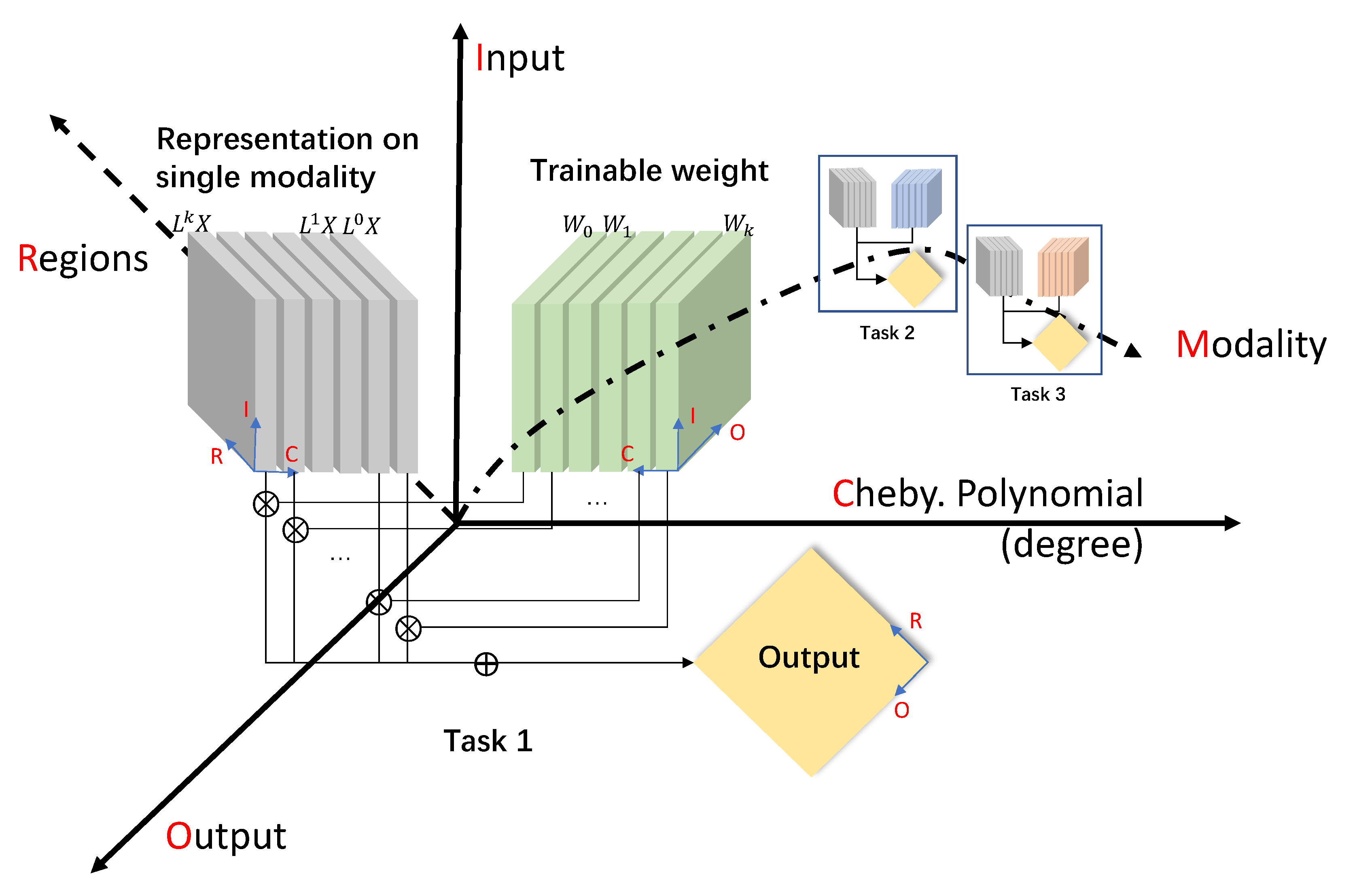
The dimensionality transformation of graph convolution operations in ChebNet is shown in Figure 4. There are five dimensions in the whole system in total, including regions/vertices (R, $\left|R\right|=\left|V\right|$), inputs (I), outputs (O), Chebyshev Polynomial (C, $\left|C\right|=K$) and modalities (M). For each single modality task, the representation of input signals on graph laplacian $L_i$ is in a three-dimensional space of region, input and Chebyshev polynomial: $\left\{L_i^{\alpha }X\right|\alpha =0,1,\dots ,K\}\in {\mathbb{R}}^{\left|V\right|\times \left|I\right|\times K}$. The model parameter for the ith modality is in a three-dimensional space of input, output and Chebyshev polynomial: $W_i^l=\left\{w_{i,\alpha }^l\right|\alpha =0,1,\dots ,K\}\in {\mathbb{R}}^{\left|I\right|\times \left|O\right|\times K}$. The joint representation for multi-modality weight is defined as a four order tensor

$$\begin{array}{c}\hfill W^l=[W_1^l,W_2^l,\dots ,W_{\left|M\right|}^l]\in {\mathbb{R}}^{\left|I\right|\times \left|O\right|\times K\times \left|M\right|}\end{array}$$

Firstly, we impose a tensor normal distribution as prior distribution for $W^l$

$$\begin{array}{c}\hfill W^l\sim \mathcal{T}{\mathcal{N}}_{\left|I\right|\times \left|O\right|\times K\times \left|M\right|}({\mathcal{M}}^l,{\Sigma }^l)\end{array}$$

(7)

where ${\mathcal{M}}^l$ is the mean tensor. ${\Sigma }^l={\Sigma }_I^l\otimes {\Sigma }_O^l\otimes {\Sigma }_C^l\otimes {\Sigma }_M^l$ is the Kronecker decomposable covariance structure. The density function is estimated as:

$$\begin{array}{c}\hfill p\left(W^l\right)=2{\pi }^{-\frac{{\prod }_{k=1}^4{d}_k}{2}}(\prod _{k=1}^4|{\Sigma }_k{|}^{-\frac{{\prod }_{k=1}^4{d}_k}{2d_k}})\times e^{-\frac{1}{2}{(W^l-{\mathcal{M}}^l)}^T{\Sigma }^{-1}(W^l-{\mathcal{M}}^l)}\end{array}$$

(8)

where $d=\left[\right|I|,|O|,K,|M\left|\right]$ and represents dimensions for each mode, $\Sigma =[{\Sigma }_I^l,{\Sigma }_O^l,{\Sigma }_C^l,{\Sigma }_M^l]$. $|·|$ represents the determinant. According to Long et al. [10], for Maximum-a-Posteriori (MAP) estimation for model parameters, learning the posterior distribution of $W^l$ given training data $(X,Y)$ is equivalent to minimizing the negative logarithm for the density of ${\prod }_{l}P\left(W^l\right)$, where (ignores terms irrelevant to $W^l$ because they have no gradient during back propagation):

$$\begin{array}{c}\hfill J_2^l=\frac{1}{2}\left(vec{\left(W^l\right)}^T{\left({\Sigma }^l\right)}^{-1}vec\left(W^l\right)\right)\end{array}$$

(9)

where $vec(·)$ is the flattening operation to transform a high-dimensional tensor to a 1-d vector. The flip-flop algorithm for updating the covariance matrix of a certain mode ${\Sigma }_i$ is:

$$\begin{array}{c}\hfill {\Sigma }_{d_i}^l=\frac{d_i}{{\prod }_{k=1}^4{d}_k}{\left(W^l\right)}_{\left(i\right)}\left({\otimes }_{k\ne i}{\Sigma }_k\right){\left(W^l\right)}_{\left(i\right)}^T+ϵI_{d_i}\end{array}$$

(10)

where $ϵI_{d_i}$ is a trade-off term for numerical stability. ${\left(W^l\right)}_{\left(i\right)}$ is the vectorization along the ith mode. Such operation outputs a matrix of shape ${\mathbb{R}}^{\left(d_i\right)\times ({\prod }_{k\ne i}{d}_k)}$

We further discovered that the covariance update rule above should not be applied to input (I) and output (O) modes. Instead, freezing the covariance matrix of input (I) and output (O) mode to the identity matrix $I_d$ will improve model generality and transferability.

Observing Equation (2) of ChebNet on the lth layer:

$$G_W(X^l;A)=\sum _{\alpha =0}^K{L}^{\alpha }{X}^l{W}_{\alpha }$$

(11)

where $L^{\alpha }{X}^l\in {\mathbb{R}}^{\left|V\right|\times f_1}$, $W\in {\mathbb{R}}^{f_1\times f_2}$, usually $\left|V\right|>>f_1>f_2$ is due to two facts:

• |V| is very large. $L^{\alpha }{X}^l$ is usually sparse.
• In higher layers of DNNs, the feature dimension is usually decreasing, i.e., $f_1>f_2$.

According to lemma on matrix multiplication:

Lemma 1.

For matrix multiplication $B=AW$, Rank $\left(B\right)$$\le \min \left\{Rank\right(A),Rank(W\left)\right\}$.

The rank for GCN output feature matrix is bounded:

$$\begin{array}{cc}\hfill & Rank\left(G_W(X^l;A)\right)\le min\{Ran{k}_{\left|V\right|}\left(L^{\alpha }{X}^l\right),\hfill \\ & Ran{k}_{|f_1|}\left(L^{\alpha }{X}^l\right),Ran{k}_{|f_1|}\left(W_{\alpha }\right),Ran{k}_{|f_2|}\left(W_{\alpha }\right)\}\hfill \end{array}$$

where $Ran{k}_{|f_2|}\left(W_{\alpha }\right)$ is the rank on the $f_2$ mode of matrix $W_{\alpha }$. Increasing the $Rank\left(W_{\alpha }\right)$ on both modes ($f_1$ and $f_2$) will lift the upper bound of the output rank. It is known that the co-adaptation problem [30] limits the generality and transferability of DNNs. Initializing and freezing the covariance matrix along the input and output dimension to $I_I$ and $I_O$ will induce a high rank matrix $W_{\alpha }$, which lifts the upper bound of rank of output features. The inter-neuron dependency is smaller for a high rank output feature matrix, so that the co-adaptation problem is alleviated and model generality is increased.

3.3. Multi-Modality Fusion

The final layer is the modality fusion layer in order to aggregate features from different modalities and output a prediction result. For a one-step spatiotemporal prediction problem, the output shape is $R^{\left|V\right|\times 1}$. The design of the modality fusion is straightforward. First, we make sure the last MRGCN layer reduces the feature dimension to 1. Then, the modality fusion layer is designed as a modality-wise average:

$$\begin{array}{c}\hfill O^{l+1}=\frac{1}{\left|M\right|}\sum _{j=1}^{\left|M\right|}{X}_j^l,X_j^l\in {\mathbb{R}}^{\left|V\right|\times 1}\end{array}$$

3.4. Training Algorithm

We combine all loss functions and summarize it for the entire network:

$$\begin{array}{cc}\hfill J_W(X,Y)=& \sum _{s\in S}{J}_0(f_W\left(x_s\right),y_s)+{\alpha }_{low}\sum _{l\in L_{low}}{J}_1^l+{\alpha }_{high}\sum _{l\in L_{high}}{J}_2^l\hfill \\ \hfill =& \sum _{s\in S}\frac{1}{\left|S\right|}\left|\right|f_W\left(x_s\right)-y_s{\left|\right|}_2\hfill \\ \hfill +& {\alpha }_{low}\sum _{l\in L_{low}}(\alpha \sum _{i=j}^{i,j=1,..,\left|M\right|}\left|\right|W_{i,j}^l\left|\right|+\sum _{i\ne j}^{i,j=1,..,\left|M\right|}\left|\right|W_{i,j}^l\left|\right|)\hfill \\ \hfill +& \frac{{\alpha }_{high}}{2}\sum _{l\in L_{high}}\left(vec{\left(W^l\right)}^T{\left({\Sigma }^l\right)}^{-1}vec\left(W^l\right)\right)\hfill \end{array}$$

where the $J_0$ term is the prediction loss of the model. In this work, we use the rooted mean squared error (RMSE) to measure distance between the predicted value and true value. In stacked MGCNs, we set $1,2,\dots ,l_k$-th layers to $L_{low}$ and use GGCN to construct graph interactions. The remaining layers $l_k,l_k+1,\dots$ are set to learn multilinear relationships by MRGCN. The $J_1$ terms are the GGCN regularizer for each lower layer. The $J_2$ terms are the relationship regularizer for MRGCN in the higher layers. ${\alpha }_{low}$ and ${\alpha }_{high}$ are the trade-off parameters for regularizers.

The overall training algorithm for the entire network, including GGCN and MRGCN, is shown below (Algorithm 1).

Algorithm 1 Training algorithm for GCN with interactions

Set layers $L_{low}=\{1,2,\dots ,l_k\}$ to grouped GCN Set layers $L_{high}=\{l_{k+1},\dots \}$ to multi-linear relationship GCN Initialize ${\Sigma }_d^l=I_d$, $\forall l\in L_{high}$ and $d\in \left\{\right|I|,|O|,|C|,|M\left|\right\}$ Initialize all weights repeat  Extract $(x_i,y_i)$ from training set as current training batch  Update model parameter W according to $J_W(x_i,y_i)$  Update covariance matrices ${\Sigma }_C^l$ and ${\Sigma }_M^l$, $\forall l\in L_{high}$  Evaluate current model using the validation set until converge (validation error no longer decreases for several epochs)

4. Experiments

In this section, we compare our graph interaction techniques with state-of-the-art baselines on region-level demand forecasting for ride-hailing service.

4.1. Dataset

We conducted our experiments on two real-world, large-scale ride-hailing datasets collected in two cities: Beijing and Shanghai. Both of the datasets were collected in the main city zone in 2017. We split data to training set (1 March to 31 July 2017), validation set (1 August to 31 October 2017) and test set (1 November to 31 December 2017). The POI data used for $A_S$ contains 13 primary categories, including business building, residential building, entertainments, etc. The road network data used for $A_C$ is extracted from railway, highway and subway dataset from OpenStreetMap [31].

4.2. Experiment Setting

The ride-hailing forecasting problem is a one-step spatiotemporal prediction problem to learn predictor $f:{\mathbb{R}}^{\left|V\right|\times T}\to {\mathbb{R}}^{\left|V\right|\times 1}$. According to previous works [2,3,5], we set T to 5. Physically, it means predicting the ride-hailing demand in the next time interval using the most recent three ones (closeness), the one in the same time yesterday (period) and the one in the same time last week (trend) [1]. V is the set of regions acquired by partitioning the main city zone to 1 km × 1 km rectangular grids. Under this setting, there are a total of 1296 regions in Beijing and 896 regions in Shanghai. We set 30 min as the time interval for both training data and test data. Each entry in the spatiotemporal tensor represents the number of ride-hailing demand of a certain region in 30 min.

We propose a 4-layer MGCN, where the first two layers are GGCN and the last two layers are MRGCN. The output dimensions for these layers were set to 32, 64, 32, 1. For all graph convolution operations, the max Chebyshev polynomial K was set to 4. In GGCN, the tunable $\alpha$ was set to 0.1 to maintain intra-modality properties. In MRGCN, the trade-off parameter $ϵ$ was set to $1\times {10}^{-6}$. We monitored RMSE on the validation set with early stopping. The regularizers ${\alpha }_{low}$ and ${\alpha }_{high}$ were both set to $1\times {10}^{-4}$. The neural network was implemented using tensorflow [32] and optimized using adam optimizer [33], with the learning rate as $5\times {10}^{-4}$ and the batch size as 32. All experiments were conducted in an environment with 10 GB RAM and 9 GB GPU memory of Tesla P40.

4.3. Performance Comparison

Table 1. Experiment performance in Beijing and Shanghai. The proposed approach achieves the best result among all methods.

Method		RMSE in Beijing	RMSE in Shanghai
Lower Layers	Higher Layers
STMGCN		10.78	8.30
MGCN		11.82	8.64
GGCN		9.51	8.18
$MRGC{N}_{2\Sigma }$		9.68	8.30
GGCN	Share weight	9.59	8.13
GGCN	DAN	9.48	8.02
GGCN	$MRGC{N}_{4\Sigma }$	9.47	7.92
GGCN	$MRGC{N}_{2\Sigma }$	9.31	7.88

shows experiment comparisons between the proposed methodology, variations and baselines:

• MGCN: Use one separate GCN to learn prediction task in each modality. There is no graph interaction among modalities.
• STMGCN [5]: Use RNN-based model to extract temporal features ahead of MGCN.
• Share weight: A common technique in multi-task learning. The GCN weight is shared across modalities in each layer.
• Domain adaptation network (DAN) [34]: Minimizing modality divergence by minimizing cross-modality feature divergence. The divergence used is mean maximum discrepancy (MMD).
• $MRGC{N}_{4\Sigma }$: The proposed multi-linear relationship GCN with all four covariance matrices updated.
• $MRGC{N}_{2\Sigma }$: Proposed method to freeze covariance matrices for input and output coordinates.

All proposed methods above are 4-layer MGCNs, with similar hidden feature sizes and same training configurations (learning rate, batch size, etc). We evaluated the model performance according to the prediction error (RMSE) on the test set. The epoch of converge shown in

Table 2. Number of epochs required to converge to optima or benchmark. The multi-task-based method reduced training time by at least 50%. The experiment was performed in the Beijing dataset. The best results were shown in bold.

Method		Epoch of Converge	Epoch to Break 10.78
Lower Layers	Higher Layers
STMGCN		115	115
MGCN		110	-
GGCN		130	55
$MRGC{N}_{2\Sigma }$		95	32
GGCN	Share weight	78	32
GGCN	DAN	72	24
GGCN	$MRGC{N}_{4\Sigma }$	51	25
GGCN	$MRGC{N}_{2\Sigma }$	82	27

and the

Table 3. Training speed for each model to achieve best performance in the ride-hailing demand forecasting task.

	STMGCN	GGCN	MRGCN	GGCN + MRGCN
Min training length	5 months	5 months	3 months	3 months
Training time	110 min	130 min	45 min	60 min

measures the time consumption for each model to reach its optima. Different models converged to different optima. Achieving a lower error usually costs longer training time. We set the benchmark to 10.78 in Beijing, which is the performance of baseline [5] on the same dataset.

The experiments showed the following facts. Firstly, according to the performance of GGCN, it improved the prediction accuracy for MGCN by invoking more complexity in spatial feature extraction on graphs. With the help of intra-modality transformations, spatial feature extraction was more complete and the model was more expressive. The performance improved by GGCN was even more significant than incorporating an RNN-based temporal feature extraction process (STMGCN). However, with the increment of the parameter size, the model was more prone to overfitting and required longer training time.

Secondly, MRGCN also improved model performance. Compared with GGCN, the influence on prediction error was slightly inferior. There is no significant difference in model capacity and model structure between MRGCN and MGCN. We infer that the multi-linear relationship approach improves prediction performance by improving model generality, so that $MRGC{N}_{2\Sigma }$ is less prone to overfit to the local fluctuations in the training set and overcomes the gap between the training set and test set. Multi-task learning based approaches, including share weight, DAN and MRGCN, all shortened the model training time. Among these approaches, the share weight method reduced model complexity by a factor of $O\left(\right|M\left|\right)$, which brought down the prediction performance. The performance of MRGCN and DAN were almost the same.

Thirdly, we show that freezing input and output coordinates in MRGCN is effective. Compared with $MRGC{N}_{4\Sigma }$, $MRGC{N}_{2\Sigma }$ decreases the prediction error. This validates our assumption that freezing the covariance for input and output dimension on the weight tensor may induce higher independency among neurons, which alleviates the co-adaptation problem, and thus improves model generality.

Training speed is another important factor to evaluate machine learning models. Table 3 shows the training time required to achieve the optimal performance of each model. We used the grid search to determine the minimum training length of each model. Given a larger training set than this, the model could not converge to a significantly lower validation error. Compared with the baseline, the proposed method reduces the amount of training set and the length of training time by approximately 50%. Among all tested approaches, $MRGC{N}_{2\Sigma }$ achieved the lowest prediction error on average and on test data after the 4th week. This is an important feature for industrial use. The life cycle for a more generalized model is longer, which reduces the frequency for a model update.

4.4. Model Generality

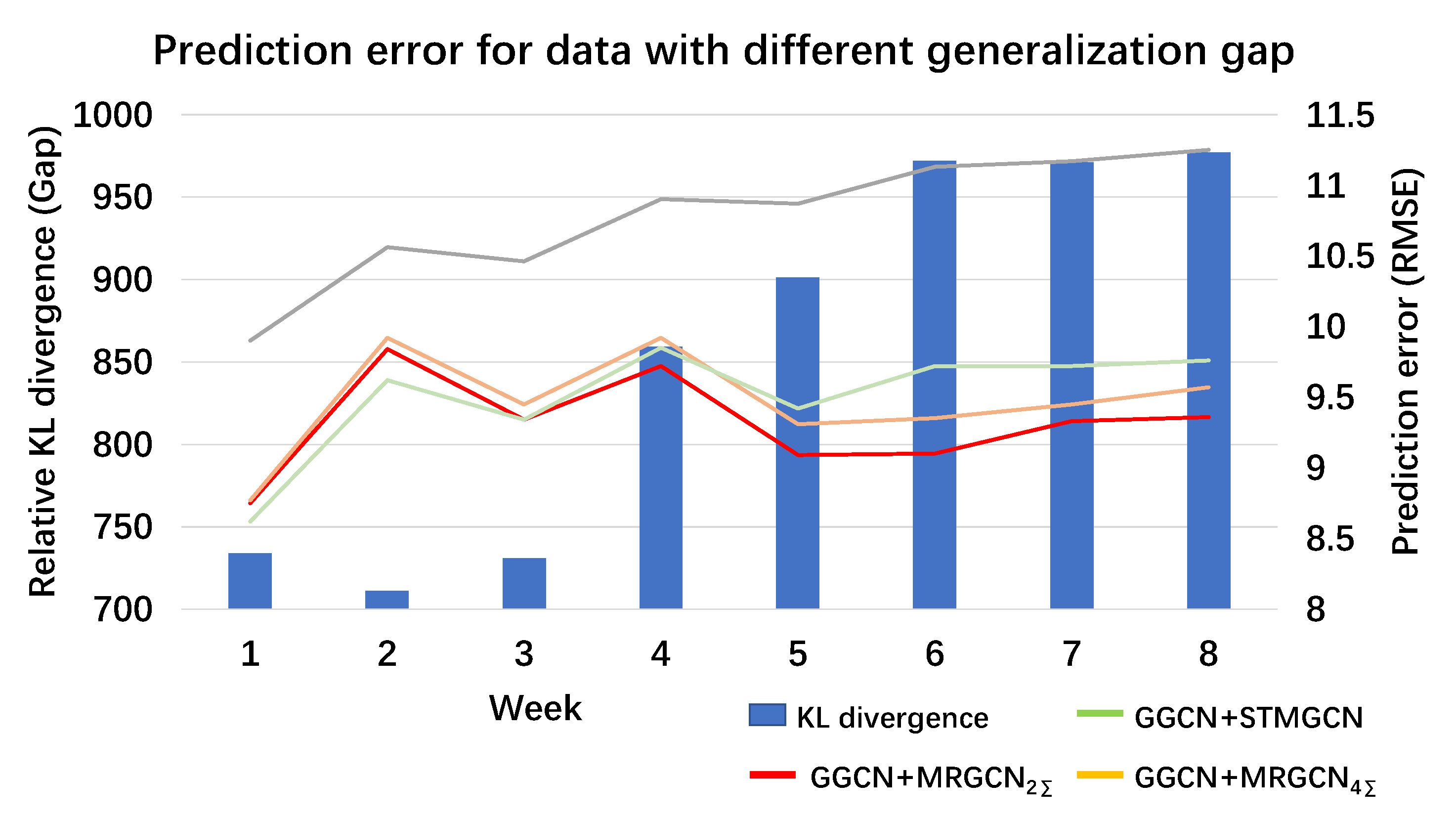
Figure 5 shows the generalization ability for different models, which validates the above arguments in detail. The data relative divergence (blue bar) was computed as the Kullback Leibler divergence [35] between the temporal pattern of the last week in the training set and temporal patterns of each week in the test set. We discovered that the gap between the training set and test set was accumulative. This indicates that the test data will become more and more divergent from the training data with time shifting. Models are expected to be more general to overcome this phenomenon. According to prediction error by weeks, the prediction error for STMGCN (the gray line) keeps increasing as the test data becomes more divergent. We believe this phenomenon is not caused by model capability, but model generality. For methods including GGCN and MRGCN, the model performance was less influenced by this generalization gap. There was no difference between the model capacity of STMGCN (MGCN) and MRGCN. The network architecture and connectivity were almost the same. This shows that MRGCN has a better generalization ability to avoid overfitting to the training set.

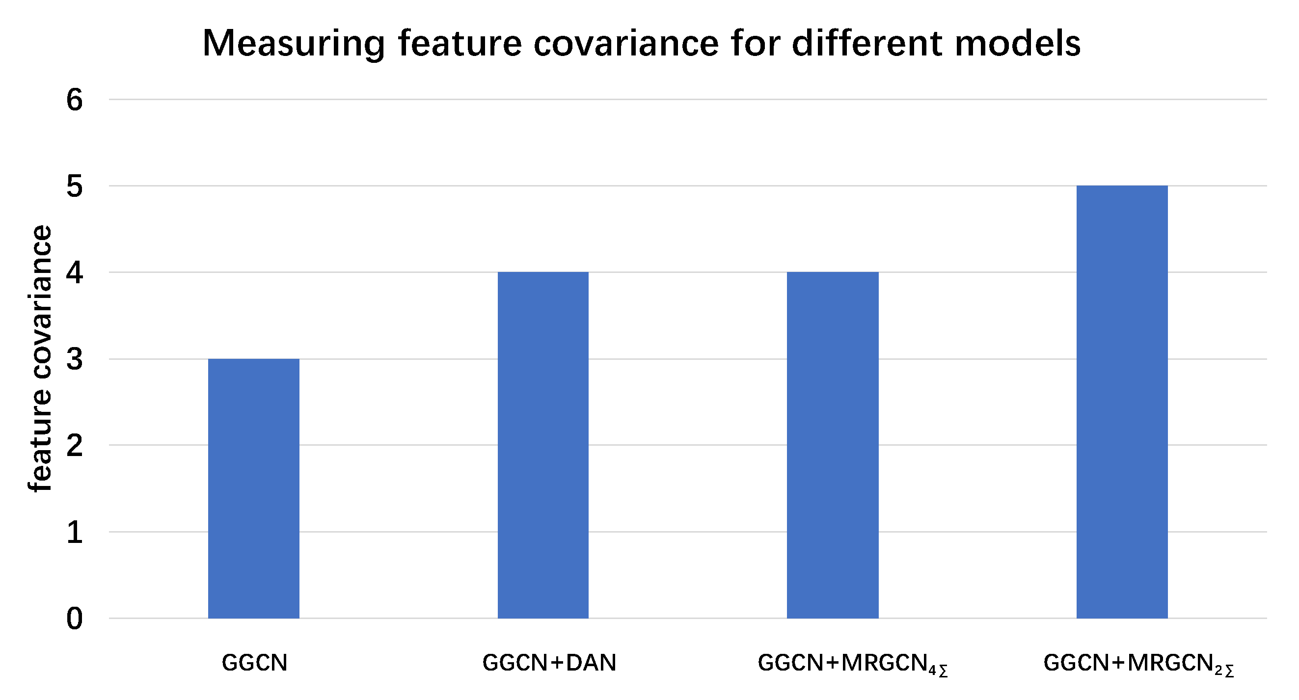
Figure 6 shows the feature inter-dependency of different models. The feature covariance is calculated as the negative logarithm of L2-norm of the covariance matrix along the feature mode. Feature covariance measures the inter-dependency between different neurons in a hidden layer of deep neural network. A higher value represents a lower absolute value for covariance between neurons and a higher neuron dependency. According to the above plot, the neuron independency could be greatly improved by MRGCN. According to Yosinski et al. [8], co-adapted neurons are the major cause for optimization difficulty in middle layers. Compared with baseline methods, the proposed $MRGC{N}_{2\Sigma }$ successfully reduced the coherence among hidden layer units and improved generality and transferability for deep neural networks.

4.5. Modality Relationship

MRGCNt learns explainable relationships between modalities by maintaining a modality-wise covariance matrix. In this part, we first show that all modalities are helpful to the learning task. Then, we will explore the relationship between the modality-wise relationship learnt from optimization and relationship between graphs.

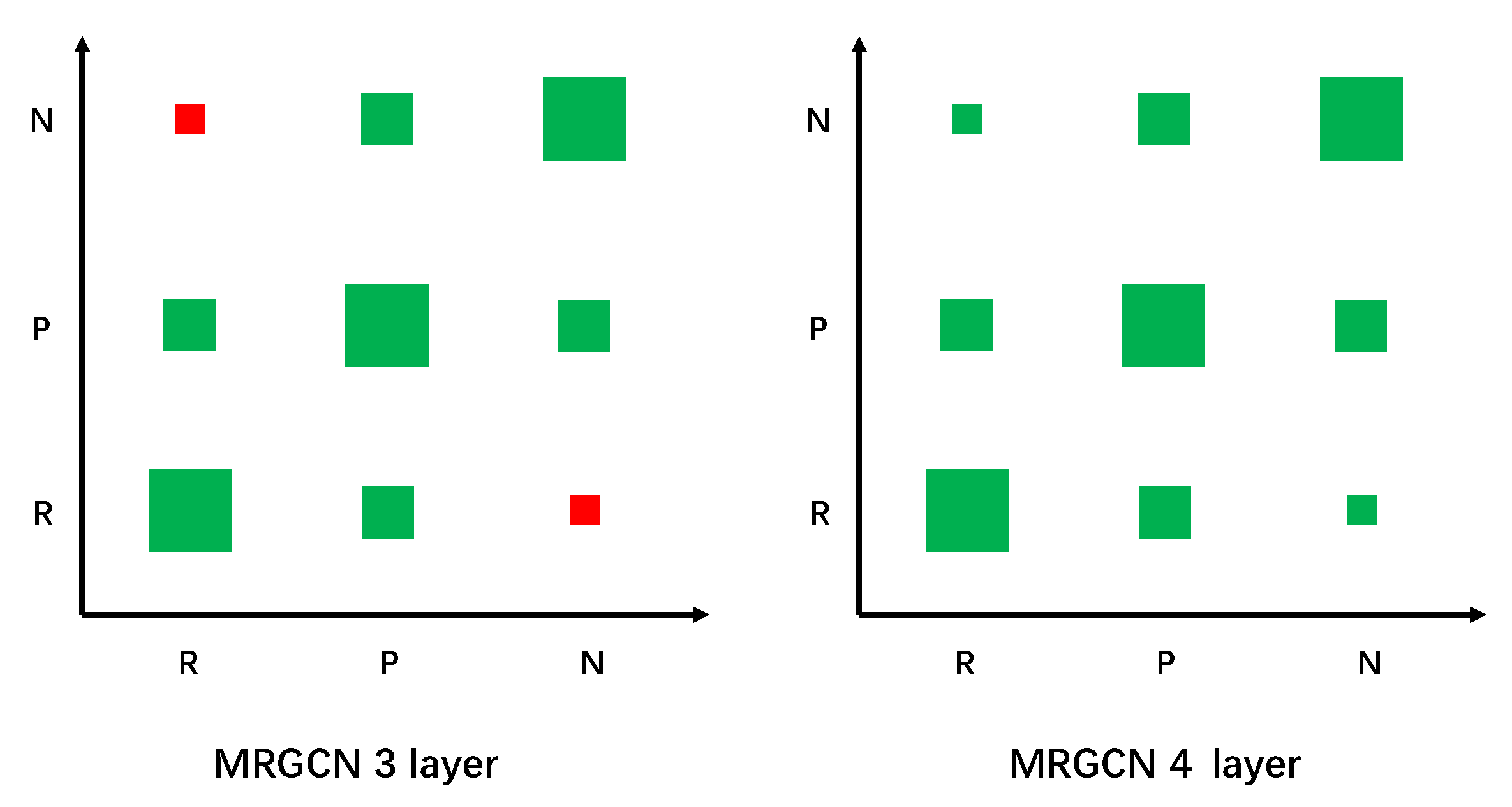
Figure 7 is the Hinton diagram showing the modality-wise relationships for the 3rd and 4th layers in GGCN+ $MRGC{N}_{2\Sigma }$. N, P, R represent modality for Neighborhood $A_N$, POI similarity $A_S$ and road connectivity $A_C$. Similar to the interpretation by [10], we could draw several conclusions. Firstly, most of the tasks are positively correlated (green), implying that all modalities could reinforce the learning of others. This conclusion reaches a consensus with ablation study [5] in

Table 4. Ablation study for ST-MGCN. Removing any one modality will result in great damage to the prediction accuracy.

Removed Component	RMSE
Neighborhood	11.47
POI similarity	11.42
Road connectivity	11.69
ST-MGCN	10.78

.

Secondly, we discovered that the relationship between N and R was weak and random. These two tasks were seemingly related. Compared with that, the relationship R-P and N-P were stable and robust. We try to explain this phenomenon by comparing the graphs $A_N$, $A_S$ and $A_C$.

Table 5. The density of each graph. The graphs are undirected. Density is calculated as $2\left|E\right|/\left|V\right|\left(\right|V|-1)$.

${\mathit{A}}_{\mathit{N}}$	${\mathit{A}}_{\mathit{S}}$	${\mathit{A}}_{\mathit{C}}$
$1.3\times {10}^{-3}$	1.4	$1.4\times {10}^{-3}$

shows the density of each graph, which measures the connectivity of the graph in each modality. According to the graph definition, $A_S$ is defined as POI similarity between any region pair, which induces a dense adjacency matrix. $A_N$ and $A_C$ are sparse. We measured the graph similarity by F-measure and edited distance in

Table 6. Two measurements to show similarity between different graphs. F-measurement considers matched and unmatched edges proportional to graph size. Edit distance measures difference between two edge sets.

	${\mathit{A}}_{\mathit{N}}$-${\mathit{A}}_{\mathit{S}}$	${\mathit{A}}_{\mathit{S}}$-${\mathit{A}}_{\mathit{C}}$	${\mathit{A}}_{\mathit{C}}$-${\mathit{A}}_{\mathit{N}}$
F-measure	0.15	0.17	0
Edit distance	$1.1\times {10}^6$	$1.1\times {10}^6$	$8.8\times {10}^2$

. According to the graph definition, edges in $A_N$ are all removed from $A_C$, so that the edge set $E_N\bigcap E_C=\varnothing$. From the view of graph connectivity, the prediction task on these modalities were hardly related. The relationship $A_S$-$A_C$ and relationship $A_S$-$A_N$ were quite similar because $A_S$ was dense. The analysis above helps to understand Figure 7. The relationship between neighborhood (N) and road connectivity (R) was quite random due to the inherent independency between these two modalities. MRGCN learns similar modality relationships for similar graph-pairs. The relationship N-P and R-P were maintained to be similar in both layers.

5. Conclusions and Future Work

In this work, we propose two graph interaction techniques for multi-modal multi-graph convolution networks. We use GGCN in lower layers to complete graph connectivity for better spatial feature extraction by graph convolution networks. In higher layers, we use MRGCN to learn robust modality relationships. MRGCN alleviates the co-adaptation problem by lifting the upper bound for feature dependency and thus improves the model generality. The experiment on ride-hailing demand prediction shows that our proposed model outperforms baselines in effectiveness, efficiency and robustness. For future work, we plan to investigate the following aspects: (1) evaluate the model with other spatial temporal prediction tasks and other region-wise relationships and (2) explore the impact of sparse and dense graphs on this framework.