1. Introduction
1.1. Background
Rear-end crashes account for a considerable portion of total crashes. According to the data reported, rear-end collisions account for 30–40% of all crashes, making them the most frequent type of traffic crashes on the freeway [
1,
2]. Rear-end crash risk has been modelled and calibrated from various sources of data. Crash data can reveal the frequency and severity of crashes. However, there are certain drawbacks to using crash data in freeway safety evaluations. It will take years to obtain enough crash data. The crash data do not include the events with high collision risk which did not lead to a crash [
3]. Furthermore, the crash data record was mostly about the time, location, casualty, and so on, and the driving details before the crash were missing.
In contrast, surrogate safety indicator, which is highly related with crash occurrence, is becoming more and more popular in recent years and can be collected in a short time [
4]. Modeling rear-end collisions using surrogate indicator rather than crash data has received increased attention [
5]. Different from the crash-based studies, surrogate safety measures can also detect the risky condition before a real crash. It was estimated based on the vehicle’s speed, acceleration, and the spacing between following and leading vehicle.
1.2. Research Gap
Although a lot of research about the surrogate indicator and rear-end collision risk has been performed in the traffic safety evaluation, there were still some limitations in common, which could influence the model performance for the practical use.
For the existing surrogate indicators, the deceleration of the leading vehicle was selected as the maximum deceleration the road surface can provide to calculate the probability of the rear-end collision, which was inconsistent with the actual situation [
6]. The braking deceleration occurred randomly, and the probability of applying maximum deceleration was very low.
Compared to the normal traffic flow, traffic crashes were in the minority. The majority of the traffic flow was safe, which resulted in an unbalanced data set. The unbalanced classification posed a challenge for the machine learning algorithms. The machine learning assumed that there was an equal number of examples for each class [
7], which may result in poor predictive performance, specifically for the minority class. As a consequence, it might lead to coarse conclusions and cannot be used in practical projects.
1.3. Objectives
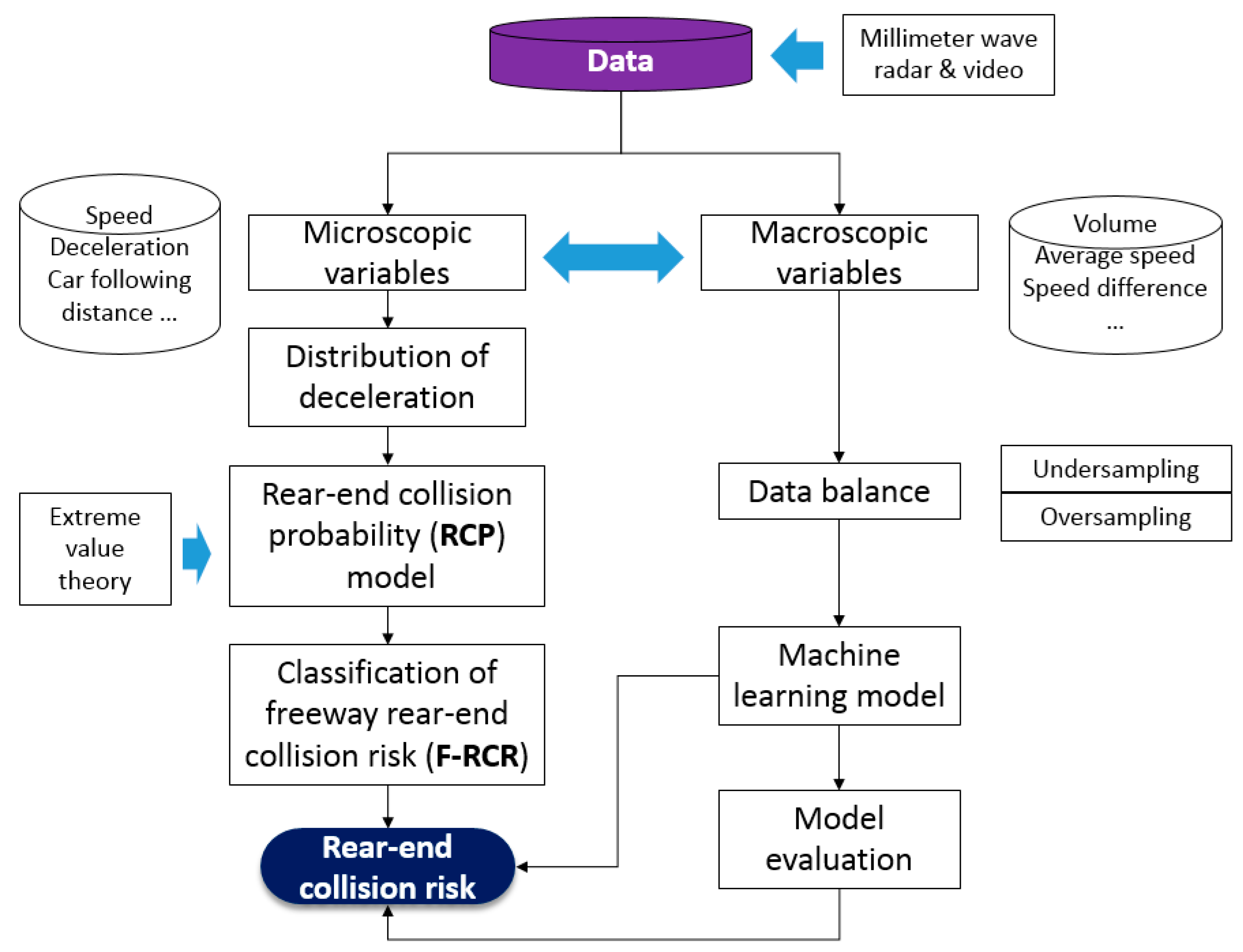
In order to fulfill the research gap, we first developed the rear-end collision probability (RCP) model based on the distribution of the deceleration. The sum of the collision probability of rear-end is defined as the freeway rear-end collision risk (F-RCR) to indicate the rear-end collision risk of the road. The F-RCR was divided into three classes, which were the high, median, and low rear-end collision probability. The high F-RCR indicates high rear-end collision risk on the freeway. Then, different machine learning algorithms were used to model the F-RCR under the condition of an unbalance dataset. The research framework is shown in
Figure 1.
The following parts of the paper were divided into six sections. Firstly, previous studies related to surrogate indicators and traffic flow risk were discussed.
Section 3 provides a brief description of the data preparation, followed by a description of the methodologies.
Section 5 presents the modeling result and discussion.
Section 6 is the conclusion of the work. Finally, the limitation and future work were also discussed.
2. Literature Review
2.1. Surrogate Indicator
The surrogate indicators can be divided into four categories, which are time, distance, deceleration, and others [
6]. Time to collision (TTC) is widely used for safety analysis, and it is the representative of time indicators. TTC defined as the time that remains until a collision between two vehicles will occur if the driving direction and speed difference are maintained. The lower the TTC is, the higher the probability of a collision will be [
6]. Based on extensions of the TTC, two new safety indicators, Exposed Time to Collision (TET) and Time Integrated TTC (TIT), were developed, which can take the full course of vehicles over space and time into account [
8]. Modified time-to-collision (MTTC) was used to estimate the conflict, and the results showed that estimated conflicts by the MTTC exhibit significant temporal and spatial correlation with real crashes [
9]. The estimated daytime conflicts were dependent on the traffic volume, and it is not sufficient for night traffic due to the limitations of MTTC to account for specific parameters such as driver distraction, drowsiness, and visibility influencing the nighttime crashes [
10]. Time to collision with disturbance (TTCD) was proposed for risk identification. TTCD can capture rear-end conflict risks in various car following scenarios, even when the leading vehicle had a higher speed. Risk rate identified by TTCD can achieve a higher Pearson’s correlation coefficient with rear-end crash rate than other traditional surrogate safety measures [
11].
Potential index for collision with urgent deceleration (PICUD) was the representative of distance indicators. It is defined as the distance between the leading and following vehicles when the leading vehicle rapidly decelerated and the following vehicle started to decelerate with a reaction delay time and stopped with urgent deceleration [
12]. A negative PICUD value implied that a crash will be occurred.
Deceleration Rate to Avoid Crash (DRAC) considered the role of speed difference and decelerations in crash occurrence. It reflected the following vehicle deceleration required to come to a timely stop or attain a matching lead vehicle speed and hence avoid a rear-end crash [
13]. Crash potential index (CPI) was developed in terms of the probability that a given vehicle DRAC exceeded its maximum available deceleration rate (MADR) or braking capability [
14]. It was found that the CPI was generally higher for the following heavy vehicle than the following car due to heavy vehicle’s lower braking capability. CPI was also validated using the simulated traffic data which replicated the observed traffic conditions a few minutes before the crash time upstream and downstream of the crash locations [
3].
Aggregated Crash Index (ACI) was proposed to measure the crash risk. This indicator reflected the accommodability of freeway traffic state to a traffic disturbance. The ACI can evaluate more car-following scenarios than the other surrogates. With a hypothetical disturbance, the proposed ACI performed well in predicting crash frequencies [
15].
2.2. Traffic Flow Risk
The development of methods for real-time traffic flow risk prediction as a function of current or recent traffic condition is popular in recent years. Different traffic states were associated with various collision types and injury severities [
16,
17]. Synchronized flow and wide moving jam were found to be the most dangerous phases. High density and low speed were associated with high crash risk [
18]. Volume, average speed, congestion index, and coefficient of variation of speed were also the main variables that affect the risk of traffic crashes [
19].
Rear-end collision risk was mainly used to reflect the safety state between the following and leading vehicle. When the risk was high, it was more likely to cause a rear-end collision. Reduced visibility had significant impact on the rear-end collision risk, and it was varied by the different vehicle types and lanes. The proportion of rear-end collision risk increased from 28.29% to 61.91% when the fog became dense [
20]. Rear-end collision risk was lower for heavy vehicles than cars in the crash case due to their shorter reaction time and lower speed when spacing is shorter. However, Meng et al. [
21] found that trucks have a much higher probability of being involved in a rear-end crash than a car at the work zone. For the rear-end collision situation, as situational urgency increased, drivers released the accelerator and braked to maximum more quickly [
22].
Rear-end collision risk was the typical unbalanced data. Only a few cases were high rear-end collision risk, most of the time was in low-risk state. Unbalanced data processing has always been one of the most important topics in machine learning. Under-sampling and over-sampling were commonly used to balance the data [
7]. The synthetic minority over-sampling technique (SMOTE) was also used to adjust the imbalanced dataset of crash and non-crash data [
19]. Under-sampled method was used to train the eXtreme Gradient Boosting model to predict real-time conflict risk [
23].
In recent days, new technologies are developing rapidly [
24,
25]. Machine learning was widely used in recent years in traffic risk detection. Stochastic Gradient Boosting (SGB), Multiple Additive Regression Trees (MARTs), and TreeNet were used to analyze crashes on the mountainous freeway. The overall model identified about 89% of crash cases in the validation dataset with only 6.5% false positive [
26]. Through the literature review, it was found that Support Vector Machine, Decision Tree, and Random Forest achieved the best performance in most of the studies presented [
24].
3. Data Collection and Accuracy
3.1. Data Collection
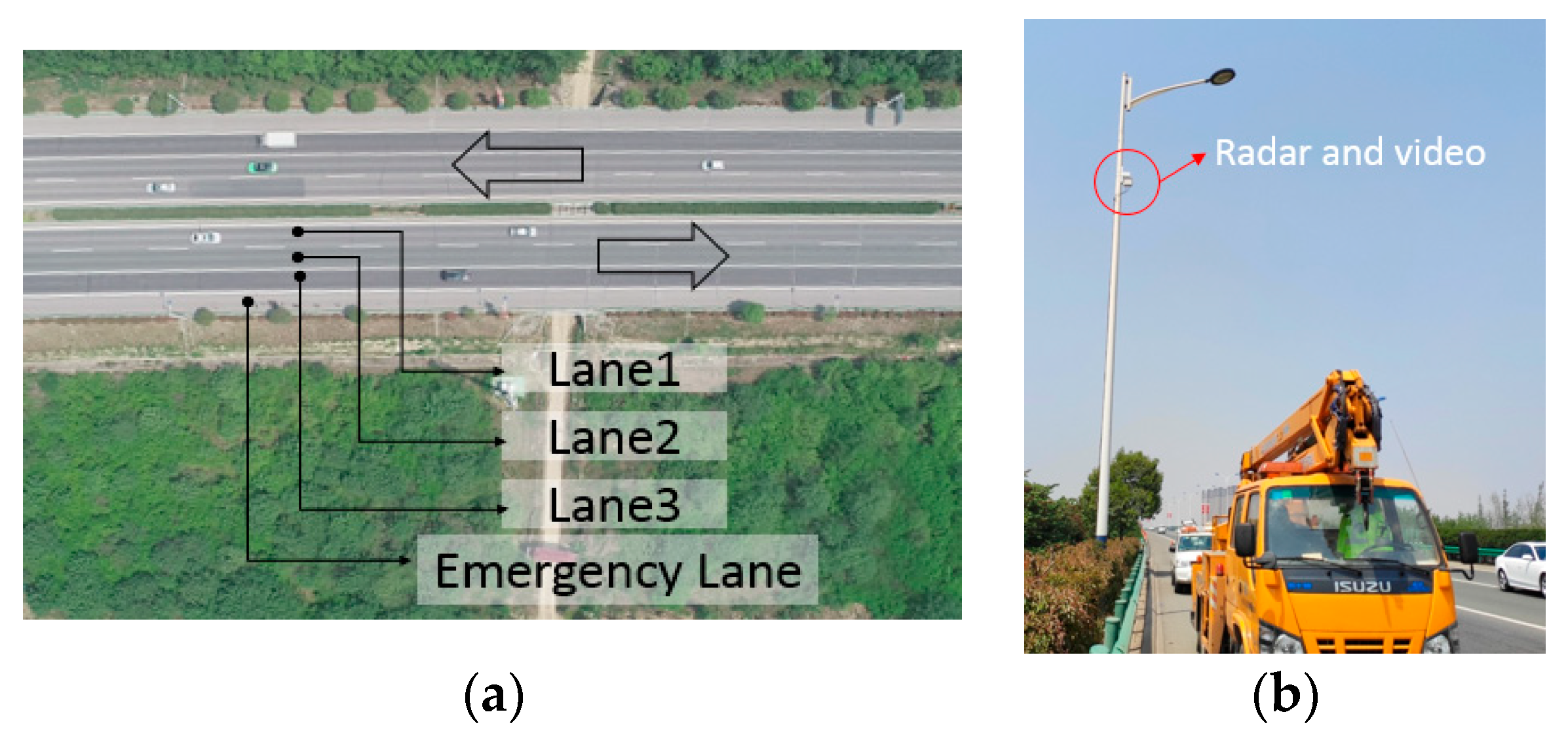
The data are crucial to the success of this study. Millimeter wave radar and video fusion equipment (MVF) is a kind of non-intrusive detection system equipment which was more and more popular in the newly constructed freeways. Millimeter wave radar is mainly used for data acquisition, and video is utilized for supplemental verification. To collect the trajectories of each vehicle, three MVFs with a height of 10 m and an average interval of 300 m were put on a roadside light pole (See
Figure 2).
A single MVF can track up to 256 vehicles at the same time, with a data acquisition every 80 milliseconds. Without the obstruction, the maximum effective tracking distance is 600 m. Small cars, on the other hand, have a weak detection effect at the far end. Only data within 300 m of a single MVF was statistically analyzed. The following data was gathered: time, vehicle ID, coordinates, vehicle type, speed, and lane number. See
Table 1 for data examples.
The length of the experiment road was about 1 km, with 3 lanes and 1 emergency lane. The lane width was 3.75 m, while the emergency lane was 2.5 m wide. The lane number was set as lane 1, lane 2, and lane 3 from left to right along the vehicle’s driving direction. Lanes 1 and 2 were primarily for passenger cars, whereas lane 3 was primarily used by heavy trucks. The speed limits on this road were 100–120 km/h in lane 1, 80–100 km/h in lane 2, and 60–100 km/h in lane 3, respectively. An aerial view of the road was shown in
Figure 2a. The daily traffic volume was about 35,000–40,000 vehicles, with passenger cars accounting for 95% of the total. The data was collected for one month from 7:00 to 20:00 during the daytime.
It should be noted that in this research we focused on the normal traffic state, and the congestion was not considered. Causes of rear-end crashes during the day and night were different [
27]. Therefore, the night was not taken into account in this study.
3.2. Data Accuracy
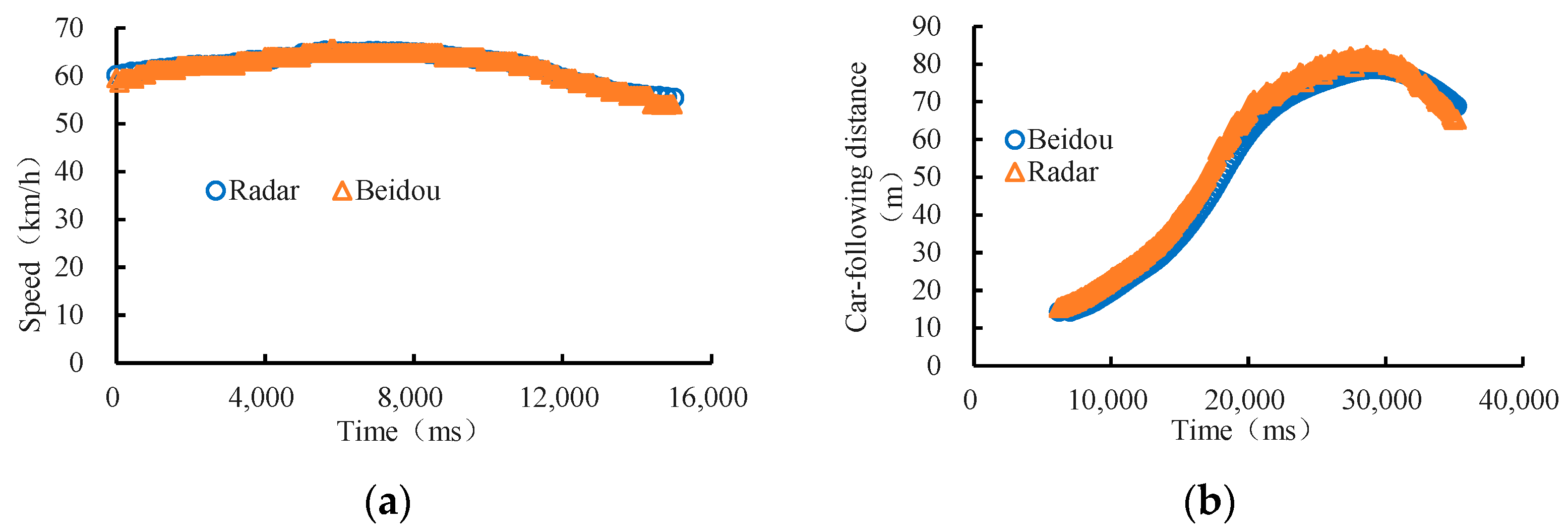
The accuracy of radar data was evaluated using Beidou satellite data. The differential positioning base station was used to improve the positioning accuracy of the Beidou satellite, which made the positioning accuracy within ±10 cm and the speed accuracy within ± 0.1 m/s.
Figure 3a shows the speed comparison between Beidou and radar. The accuracy of vehicle speed collected by radar is 99.1%.
Figure 3b demonstrates the comparison of car following distance between Beidou and radar in an experiment. The accuracy of car following distance can be as high as 92.1%. The error was mainly due to the uncertainty of the reflection point of millimeter wave on the vehicle.
4. Methodology
4.1. Modeling Vehicle Rear-End Collision Probability (RCP)
4.1.1. Vehicle Collision Analysis
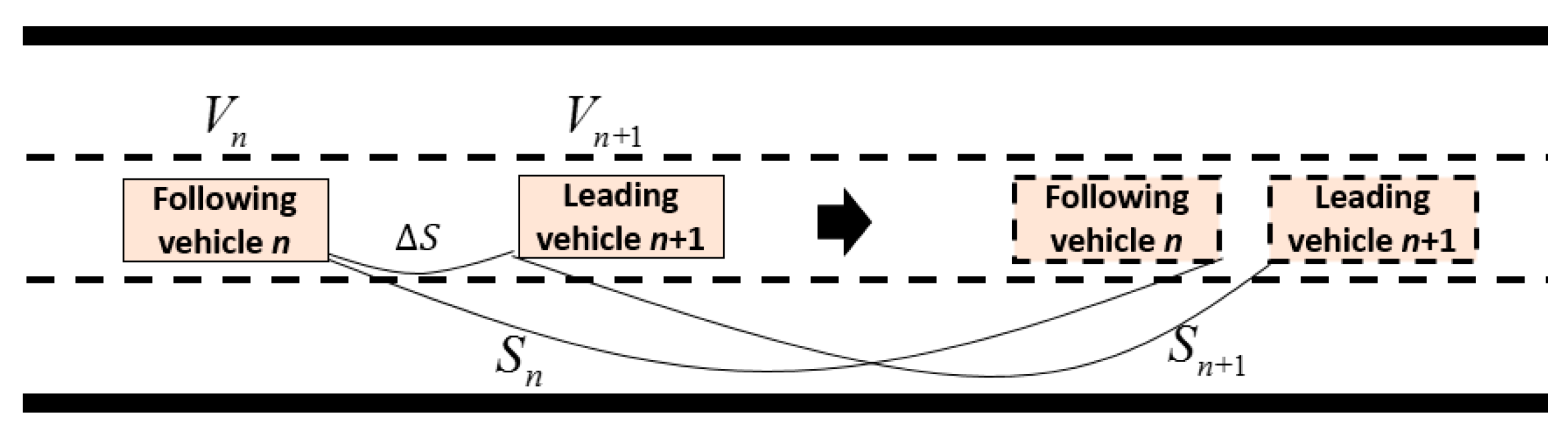
Rear-end collisions are the most common type of traffic crashes on the freeway. Therefore, this study focused on the rear-end collision on the freeway. There are three different scenarios to discuss. The driving state is shown in
Figure 4.
Case one, the following vehicle collided with the leading vehicle during the reaction time (
), that is,
where
is the speed of following vehicle
n and
t is the time from the beginning of deceleration of the leading vehicle to collision.
is the reaction time.
is the speed of the leading vehicle
n + 1;
is the deceleration of the following vehicle n.
is the deceleration of the leading vehicle
n + 1.
is the following distance between the following of the vehicle and the leading vehicle when leading vehicle braked;
is the distance traveled by the leading vehicle from the start of braking to the collision.
When the deceleration of the leading vehicle satisfies Equation (2), the following vehicle will collide with the leading vehicle within the reaction time. In an emergency, the driver released the accelerator faster and applied the emergency brake. The driver’s reaction time can be as fast as 1.2 s [
28].
Case two, after the reaction time, the following vehicle started to brake, the leading vehicle was still moving. The following vehicle collided with the leading vehicle.
is the distance traveled by the following vehicle after the reaction time when it collided with the leading vehicle.
When the deceleration of the leading vehicle meets Equation (4), a rear-end collision will occur. According to the previous study, the free lane changing duration on the freeway took about 6.09 s [
29]. So,
t was selected between 1.2 s and 6.0 s in case two.
is the maximum deceleration provided by the road. The maximum braking deceleration was different under different weather conditions. Generally,
was usually selected as 0.6 g [
6].
Case three, the leading vehicle stopped, and the following vehicle collided with the leading vehicle, that is
.
Considering the three different scenarios above, the minimum deceleration of the leading vehicle was shown in Equation (7).
is the minimum deceleration getting from Equation (7). When the deceleration of a leading vehicle was greater than or equal to , a rear-end collision would happen.
The probability of deceleration of the leading vehicle greater than or equal to
was the probability of a collision. That is:
4.1.2. Generalized Pareto Distribution Model
Extreme-value theory is a popular approach for modeling extreme values, by extracting observations that exceed a certain threshold. The distribution can be approximated by a Generalized Pareto Distribution (GPD) model [
30,
31]. In a range of industries, including insurance, flood, finance, energy, rainfall, and other natural phenomena, GPD was often utilized to model observations that exceeded a specific threshold. The distribution function of x over a threshold was defined in Equation (9).
is the shape parameter, is the scale parameter and is the threshold parameter. The GPD was often used to model the tails of another distribution. In this research, the GPD model was adopted to model distribution of deceleration.
The probability weighted moment (PWM) method, method of least squares (MLS), maximum likelihood estimation (MLE) are commonly used to estimate the GPD parameters [
32]. Kolmogorov-Smirnov (K-S) was used to test goodness of fit.
The threshold of GPD is important to the distribution. Mean Residual Life Plot and Hill-Assumption-Based Methods are used to estimate the threshold [
33].
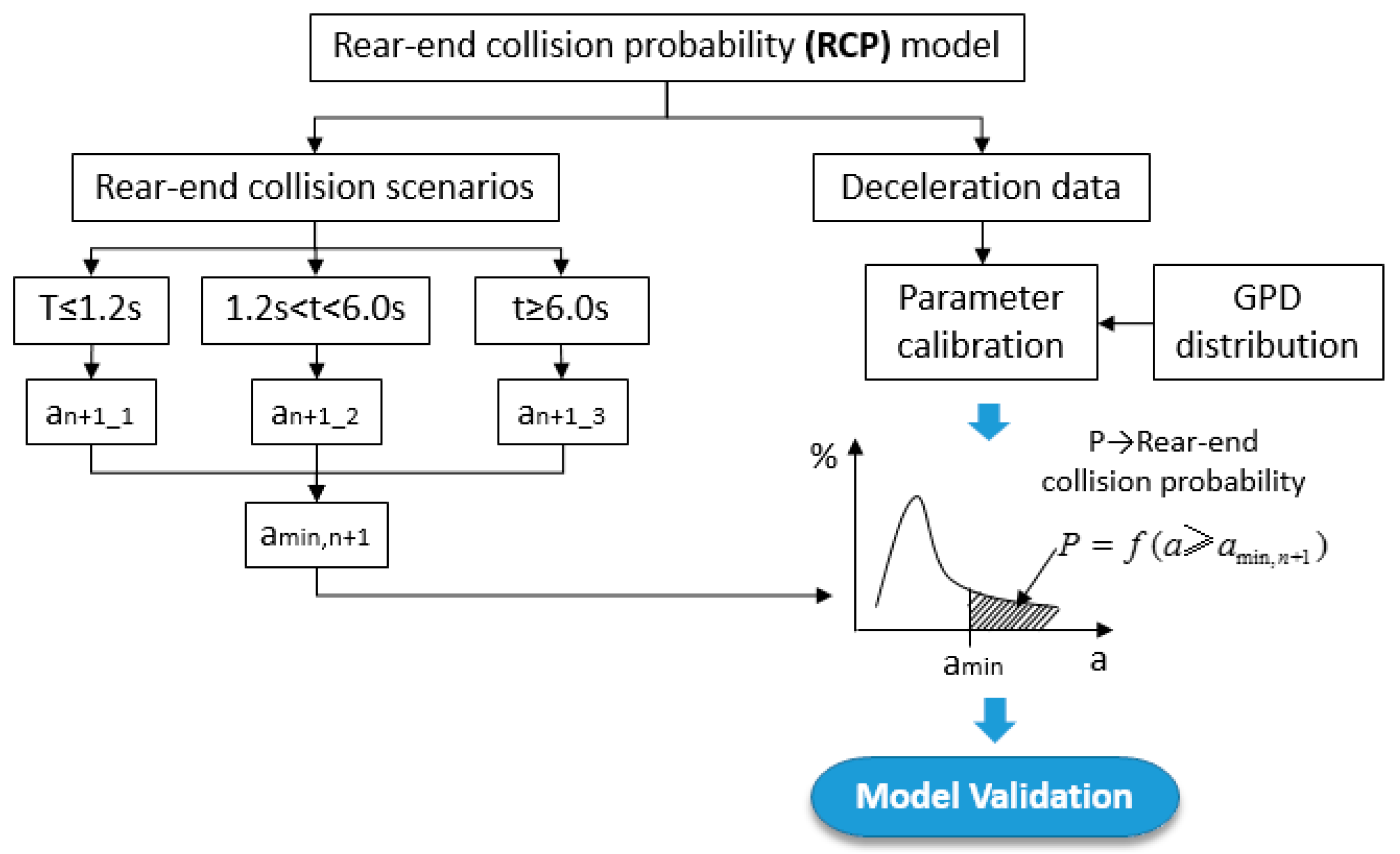
In this study, the rear-end collision scenarios were divided into three cases and GPD was used to model the tail of the deceleration distribution to calculate the RCP. The calculation process of RCP is as follows.
Step 1: Calculate the minimum deceleration required of the leading vehicle when the following vehicle collided with the leading vehicle.
Step 2: To obtain the distribution of vehicle deceleration on this road.
Step 3: To calculate the probability of the minimum deceleration. When the deceleration of a leading vehicle was greater than or equal to minimum deceleration, a rear-end collision would happen.
The framework of RCP model is shown in
Figure 5.
4.2. Modeling Freeway Rear-End Collision Risk (F-RCR)
4.2.1. Classification of F-RCR Based on Fuzzy C-Means (FCM)
The sum of each vehicle’s rear-end collision probability is defined as the freeway rear-end collision risk (F-RCR) every 100 m in five minutes. That is to say, F-RCR represents the total value of the rear-end collision probability of all the vehicles on the road within a time range. The higher the F-RCR, the higher the rear-end risk. The lower the F-RCR, the lower rear-end risk. Converting the crash risk probability to the crash risk level can directly judge the status of a crash risk under the current traffic flow condition [
34]. A reasonable F-RCR threshold was critical for the classification of high rear-end collision risk.
In most cases, the samples in the data set cannot be divided into clearly separated clusters. Compared with K-Means clustering, FCM provides more flexible clustering results. FCM was originally proposed by Bezdek [
35] based on fuzzy factors. Fuzzy C-means (FCM) is a data clustering technique in which a data set is grouped into N clusters with every data point in the dataset belonging to every cluster to a certain degree. For example, a data point that lies close to the center of a cluster will have a high degree of membership in that cluster. FCM was used to classify the traffic safety status, for example, the driving risk statuses was grouped into four different levels using FCM which were safe, low-risk, median-risk and high-risk [
36].
4.2.2. Machine Learning Model
In the fields of artificial intelligence and pattern recognition, machine learning is a major research area. In recent years, the use of machine learning techniques in traffic safety has been increasing (refer to [
24] for details). The F-RCR was modeled in this work using various machine learning models that took into account the influence of unbalanced data.
The SVM model is a kernel-based classifier and a non-parametric method for solving classification problems based on statistical learning theory. In multidimensional space, an SVM model is essentially a representation of distinct classes in a hyperplane. SVM divides datasets into classes in order to identify the maximum marginal hyperplane. Since the SVM model has been introduced in many previous research, the details were not repeated in this paper [
37,
38].
The Artificial Neural Network is based on brain and nervous system research and aims to model the behavior of biological systems made up of neurons [
24]. Two popular ANNs were compared, which were Multi-Layer Perceptron (MLP) and Radial Basis Function (RBF) networks. The MLP can be trained by a back propagation algorithm [
36]. The universal approximation and quicker learning speed of RBF networks set them apart from other neural networks (refer to [
24] for details).
Random forest (RF) is a machine learning technique that is used to solve regression and classification problems. RF is a combination of tree predictors such that each tree depends on the values of a random vector sampled independently and with the same distribution for all trees in the forest [
39]. Increasing the number of trees increases the precision of the outcome. It solves the issue of overfitting in decision trees. RF has been widely used in the traffic safety research [
40] and has been introduced in many previous research, thus the details were not repeated in this paper.
4.2.3. Macroscopic Traffic Flow Variables
Considering the practicability of the model in the future, 10 different macroscopic traffic flow variables were selected to model the F-RCR. Speed, volume, vehicle distribution, and vehicle type were mainly considered. Coefficient of variation of vehicle distribution (CVVD) showed the vehicle distribution characteristics on the freeway. It was a new variable which was not considered in the previous studies. The greater the CVVD, the more uneven the vehicle distribution. Vehicles moving in groups resulted in a greater CVVD. Every 5 min, macroscopic variables were calculated. Macroscopic traffic flow variables are shown in
Table 2.
5. Results and Discussion
5.1. RCP Model
5.1.1. Distribution of Deceleration and Model Results
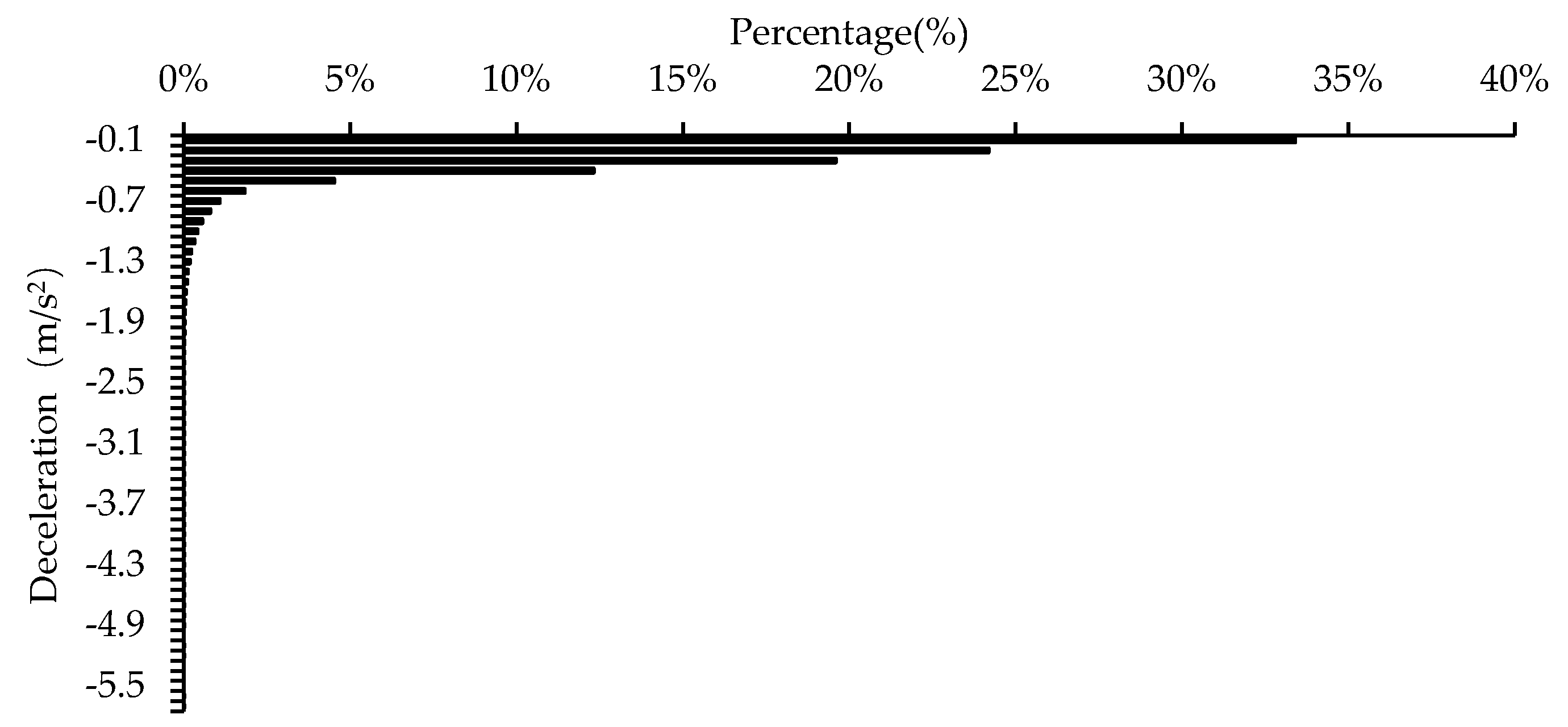
The vehicle deceleration distribution curve is shown in
Figure 6. The maximum braking deceleration was 5.6 m/s
2.
As can be seen from
Figure 6, the distribution of deceleration was very concentrated. About 30.16% of the deceleration was between [−0.1, 0.0] m/s
2, and about 95.10% of the acceleration was between [−1, 0] m/s
2. The vehicle was moving at a constant speed with a small volatility. Only in rare cases does the driver make a significant deceleration.
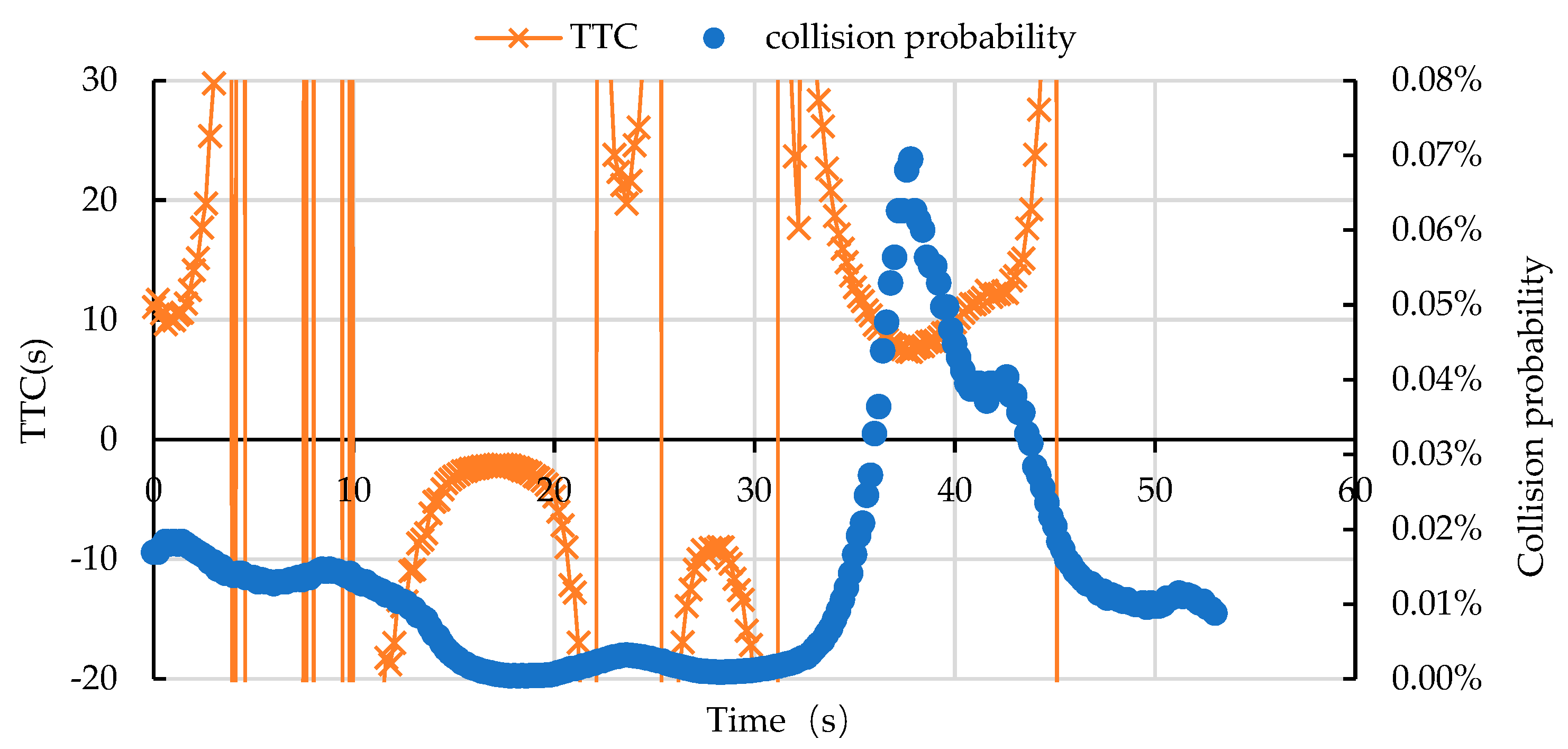
Based on the distribution of vehicle deceleration, the RCP model was developed using GPD. The model result was compared to TTC for verification. From
Figure 7, it can be seen that TTC fluctuated violently when the speed of the leading and following vehicle was close, which cannot truly reflect the dangerous driving state. The RCP model proposed in this study, on the other hand, had continuous results and can reflect the collision probability of vehicles in any car following scenario, even when the leading vehicle’s speed was equal or greater than that of the following vehicle. In consequence, the result of RCP model was more accurate. Furthermore, in contrast to traditional indications, the rear-end collision probability predicted in this paper grew rapidly in the unsafe state, enabling for real-time monitoring of dangerous traffic situations. This demonstrated that the RCP model can be used to capture rear-end collision risk on freeways.
5.1.2. Model Calibration and Validation
The small car on this road accounted for more than 95% and this study mainly focused on the collision probability of small cars. For the GPD model, the braking deceleration threshold of passenger car was 1.0 m/s2, the shape parameters and scale parameters of the passenger car were 0.0145 and 0.429, respectively. It passed the K-S test.
Naturalistic driving data was used to validate the model. This data was collected for 53 s. The vehicles were small cars. The driving speed was 80–100 km/h, the minimum car following distance was 16 m, and the maximum speed difference was 15.44 km/h. The RCP model proposed in this study was compared with TTC in
Figure 7.
Only TTC within the range of −20~30 s was shown in
Figure 7. As can be seen from
Figure 7, the effects of TTC differed substantially. This was due to the fact that relative speed had a significant impact on TTC, especially when the two vehicles’ speeds were close. However, the calculation results of RCP model proposed in this paper varied continuously. The collision probability decreased gradually in 0–15 s and approached zero in about 15–30 s. Then it increased rapidly between 30 and 38 s during which the speed of the following vehicle was higher than that of the leading vehicle, and the car following distance gradually decreased. The collision probability peaked at 37.8 s, after which the following vehicle continued to slow down and the likelihood of a collision reduced steadily. TTC was at its lowest (TTC = 7.32 s) when the collision probability was at its highest at 37.8 s. The results calculated by the two different methods were consistent at this time point.
5.2. F-RCR Model
5.2.1. Distribution of F-RCR and Classification
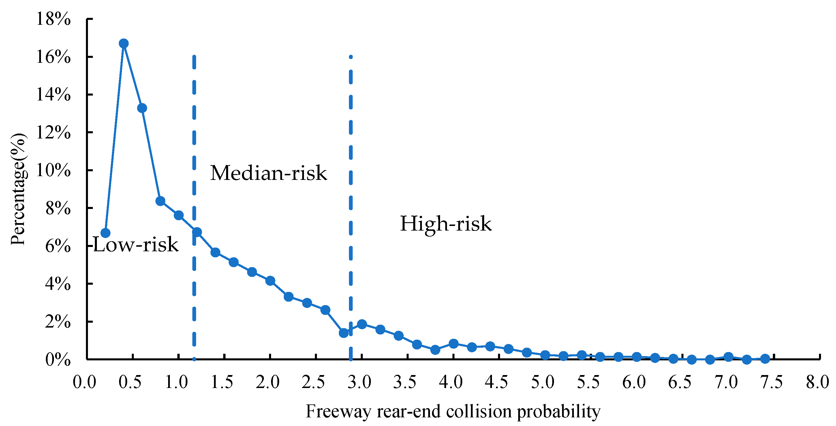
The F-RCR distribution is shown in the
Figure 8. A total of 1857 groups of data were obtained, with a total length of 1857 × 5 min = 9285 min.
As can be seen from
Figure 8, the F-RCR showed a long-tail distribution. The majority of the traffic flow was safe (low rear-end collision risk), with only a few exceptions (high rear-end collision risk). The number of warning times that traffic managers can accept is directly proportional to the magnitude of the F-RCR threshold. The smaller F-RCR threshold was, the more times of warning there were. It was not beneficial to traffic management if the number of warnings increased. The higher the threshold, the fewer the warnings, and the real dangerous situation may be overlooked. As a result, finding an appropriate F-RCR threshold required striking a balance between the two.
FCM was used to classify the F-RCR into three groups [
35], which were low-risk, median-risk and high-risk. A data point that lies close to the center of a cluster will have a high degree of membership in that cluster. FCM was used to classify the traffic safety status [
36]. The low-risk state was the safe state and the high-risk state was the risky state which was related with the rear end crashes. The low-risk, median-risk, and high-risk accounted for 52.72%, 36.70%, and 10.58%, respectively. The low-risk and median-risk ranged from 0 to 1.17 and 1.17 to 2.88. On the other hand, the high-risk was above 2.88.
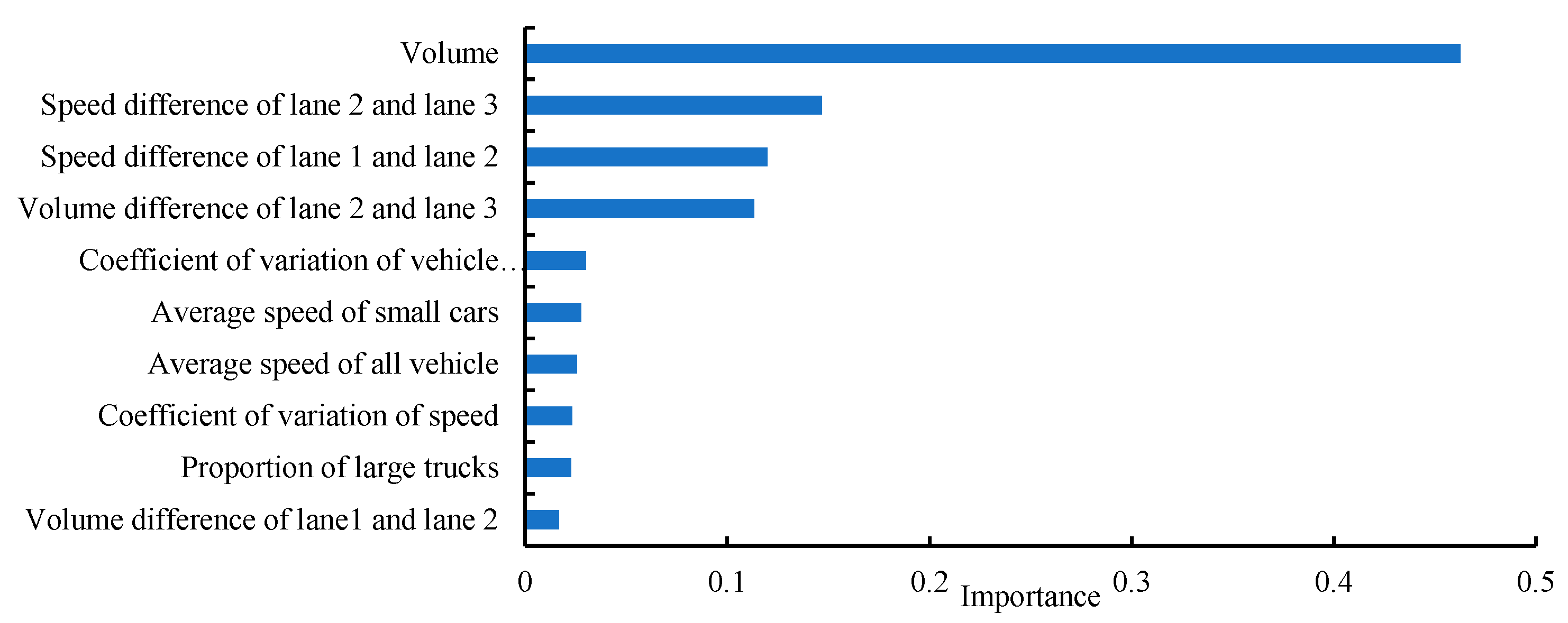
5.2.2. Variable Importance
The importance of macroscopic traffic flow parameters for the F-RCR was calculated using the SVM model, and the results were shown in
Figure 9. The results showed that the traffic volume had the greatest influence on the F-RCR. The greater the volume, the smaller the car following distance, the more prone to rear-end collisions, resulting in a rise of the F-RCR. It was consistent with the previous studies, in which was found that the AADT indicator played a critical role for the rear-end collision [
41].
The second influencing factor was the speed difference between adjacent lanes, which mainly included the speed difference between lane 2 and lane 3, as well as the speed difference between lane 1 and lane 2. When the speed gap between adjacent lanes is large, drivers will change lanes to obtain a better driving environment. During the process of lane changing, there was always a large speed difference [
29], which increased the likelihood of a collision. Shangguan [
36] also found that speed difference was an important factor for the driving risk status which was consistent with the result of this research.
The third influencing factor was the coefficient of variation of vehicle distribution (CVVD). The CVVD reflected the fluctuation of vehicle distribution, that was, the uneven distribution of vehicles on the freeway. Especially when vehicles were moving forward in the form of vehicle groups, resulting in an increase in CVVD. When the vehicle moving in the form of vehicle groups, the car following distance was short and the rear-end collision risk was increased.
Finally, it can be concluded that when the vehicle distribution was uneven, the speed difference between adjacent lanes was large, and the traffic volume was large, the F-RCR will increase.
5.2.3. Machine Learning Model
The data was split into two groups: the training data set (60%) and test data set (40%). Based on the mixed sampling, which is the combination of the oversampling and under-sampling method, the calculation results of the test data of different models are shown in
Table 3.
It can be seen from
Table 3, the low-risk had the highest accuracy. The results of the low-risk of the three models were all above 90%. The accuracy of the median-risk and high-risk were all over 80% indicating that the model performed well in general.
High-risk was the minority data which accounted for less than 10% of all the data. The accuracy of the minority data set was of great interest. The cost of misjudgment of high-risk (minority class, high rear-end collision risk) was substantially higher than that of low-risk (majority class, low rear-end collision risk). It was desirable to give high prediction accuracy over the high-risk (minority class), although adequate accuracy for the safe state was also desired (majority class). The high-risk result of the MLP, RBF, and RF was 86.4%, 83.3%, and 84.4%, respectively. MLP was shown to be more appropriate for modeling the rear-end collision risk on the freeway, which was consistent with previous studies [
42]. However, some other studies showed that RF obtained the best performance [
24,
43], which is mainly because the research topic was different. The previous studies modelled the crash injury severity which was different from the rear-end crash risk in this paper.
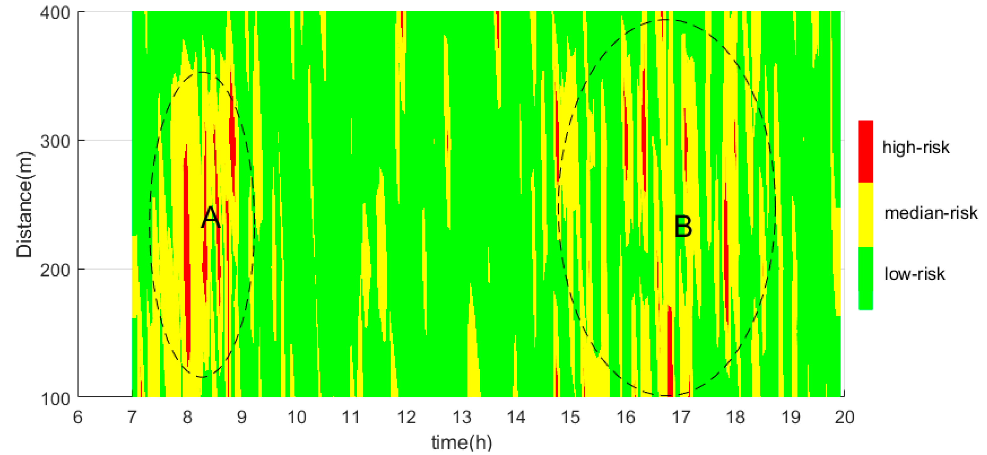
5.3. Case Study
The data from 7:00 a.m. to 8:00 p.m. was collected in one day and the weather condition was good. The freeway was located outskirts of the city. The length of the experiment road was 500 m. The F-RCR was calculated in five minutes every 100 m. The F-RCR was classified into 3 levels based on the FCM. The result of the F-RCR was showed in
Figure 10.
Figure 10 shows that it was low-risk status at most of the time. There has been a high-risk in section A and B, which time was from 7:00–9:00 a.m. and 15:00–19:00 p.m. In the morning peak hours, the traffic volume increased and the morning commute was very concentrated. It became low risk immediately after 9 a.m. for the working time was 9 o’clock. The section B can be regarded as evening peak hours and traffic volume increased. Compared with section A, the high-risk distribution in section B was more discrete. Larger volume variation between lanes will increase crash occurrence likelihood. This was consistent with previous studies that the crash rate would be increased when the volume increased [
44] and larger volume variation between lanes [
45].
High-risk was surrounded by median-risk which showed that the result was reasonable for the changing of the F-RCR was continuous. The F-RCR cannot change immediately from low-risk to high-risk without median-risk.
6. Conclusions
Rear-end crash is the most common crash type on the freeway. This paper provides an alternative framework for assessing the rear-end collision risk on the freeway. It showed the potential to be used in the active traffic management system, especially for the proactive safety solutions.
Firstly, the rear-end collision probability (RCP) model for the two vehicles was developed based on the GPD model. Secondly, the sum of all the vehicle rear-end probability on the freeway was defined as the freeway rear-end collision risk (F-RCR). Then, the F-RCR was divided into three classes which were high, median, and low rear-end collision risk. Different machine learning algorithms were used to model the F-RCR, especially the high rear-end collision risk.
For the RCP model, the distribution of vehicle deceleration was considered, which corresponded with the actual situation. The result of RCP model was more accurate, and it can quickly detect the dangerous scenarios. The RCP model, unlike the traditional surrogate indicators, can be used in a variety of car-following scenarios even when the speed of the leading vehicle is faster than the following vehicle. Furthermore, after the model parameters have been calibrated, RCP model can be used on different sections of roads, for example, the freeway interchange.
For the F-RCR, it was modelled by different machine learning algorithms and the impact of unbalanced data on the model was considered. For the machine learning model evaluation, the prediction accuracy of the high rear-end collision risk was the first consideration, followed by the overall accuracy. It was concluded that MLP has the best prediction result. When the vehicle distribution was uneven, the speed difference between adjacent lanes was large, and the traffic volume was large, the F-RCR will increase.
The macroscopic variables of the machine learning model were easy to get. The model provided in this study is transferrable after parameter calibration. Therefore, it can be applied to real-world traffic management and can also be used as part of any traffic safety evaluation that compared before and after traffic measures. For example, the benefits of ATM operations or any other ITS implementations.
7. Limitations and Future Work
This research collected data at the freeway straight section for one month to model the F-RCR. The road section contains three general traffic lanes in one direction. However, in some developed areas, more and more freeways with four traffic lanes or even five lanes in one direction were constructed, which would lead to more complex traffic behavior. To improve model performance, additional data should be collected on various road types as well as in various weather conditions. The RCP model was compared using the traditional surrogate indicator TTC. A large-scale validation study should be carried out based on the crash data to validate and improve the model prediction result.
Since the percentage of small cars in the study site was greater than 95 percent, only the rear-end collision probability of small cars was investigated. The deceleration behavior of heavy trucks were quite different from the small cars [
3]. Heavy trucks should also be emphasized in the further research.
The high F-RCR accounted for about 10% of the data set which was typical unbalance data set. Most machine learning classification algorithms were sensitive to unbalance data. To improve the predicted accuracy of machine learning model under the condition of unbalanced data was also the future research direction.
Author Contributions
Conceptualization, X.M.; methodology, X.M.; formal analysis, X.M.; writing—original draft preparation, X.M.; writing—review and editing, Q.Y.; supervision, Q.Y.; funding acquisition, J.L. All authors have read and agreed to the published version of the manuscript.
Funding
This study was sponsored by National Key R&D Program of China [2017YFC0803900].
Institutional Review Board Statement
Not applicable.
Informed Consent Statement
Not applicable.
Data Availability Statement
The data used in this study are available from the corresponding author upon request.
Conflicts of Interest
The authors declare that there are no conflict of interest regarding the publication of this paper.
References
- Xi, J.; Guo, H.; Tian, J.; Liu, L.; Sun, W. Analysis of Influencing Factors for Rear-End Collision on the Freeway. Adv. Mech. Eng. 2019, 11, 1687814019865079. [Google Scholar] [CrossRef]
- Wen, J.; Wu, C.; Zhang, R.; Xiao, X.; Nv, N.; Shi, Y. Rear-End Collision Warning of Connected Automated Vehicles Based on a Novel Stochastic Local Multivehicle Optimal Velocity Model. Accid. Anal. Prev. 2020, 148, 105800. [Google Scholar] [CrossRef] [PubMed]
- Zhao, P.; Lee, C. Assessing Rear-End Collision Risk of Cars and Heavy Vehicles on Freeways Using a Surrogate Safety Measure. Accid. Anal. Prev. 2018, 113, 149–158. [Google Scholar] [CrossRef]
- Park, H.; Oh, C.; Moon, J.; Kim, S. Development of a Lane Change Risk Index Using Vehicle Trajectory Data. Accid. Anal. Prev. 2018, 110, 1–8. [Google Scholar] [CrossRef]
- Golob, T.F.; Recker, W.W.; Alvarez, V.M. Freeway Safety as a Function of Traffic Flow. Accid. Anal. Prev. 2004, 36, 933–946. [Google Scholar] [CrossRef] [PubMed]
- Mahmud, S.M.S.; Ferreira, L.; Hoque, M.S.; Tavassoli, A. Application of Proximal Surrogate Indicators for Safety Evaluation: A Review of Recent Developments and Research Needs. IATSS Res. 2017, 41, 153–163. [Google Scholar] [CrossRef]
- Li, X.; Zhang, L. Unbalanced Data Processing Using Deep Sparse Learning Technique. Future Gener. Comput. Syst. 2021, 125, 480–484. [Google Scholar] [CrossRef]
- Minderhoud, M.M.; Bovy, P.H.L. Extended Time-to-Collision Measures for Road Traffic Safety Assessment. Accid. Anal. Prev. 2001, 33, 89–97. [Google Scholar] [CrossRef]
- Ozbay, K.; Yang, H.; Bartin, B.; Mudigonda, S. Derivation and Validation of New Simulation-Based Surrogate Safety Measure. Transp. Res. Rec. 2008, 2083, 105–113. [Google Scholar] [CrossRef]
- Charly, A.; Mathew, T.V. Estimation of Traffic Conflicts Using Precise Lateral Position and Width of Vehicles for Safety Assessment. Accid. Anal. Prev. 2019, 132, 105264. [Google Scholar] [CrossRef]
- Xie, K.; Yang, D.; Ozbay, K.; Yang, H. Use of Real-World Connected Vehicle Data in Identifying High-Risk Locations Based on a New Surrogate Safety Measure. Accid. Anal. Prev. 2019, 125, 311–319. [Google Scholar] [CrossRef] [PubMed]
- Suzuki, K.; Imada, K.; Matsumura, Y. A Study of Collision Risk Estimation and Users Evaluation at Merging Section of Urban Expressway in Japan. Transp. Res. Procedia 2016, 15, 783–793. [Google Scholar] [CrossRef]
- Cunto, F.; Saccomanno, F.F. Calibration and Validation of Simulated Vehicle Safety Performance at Signalized Intersections. Accid. Anal. Prev. 2008, 40, 1171–1179. [Google Scholar] [CrossRef]
- Craveiro, F.C.J.; Saccomanno, F.F. Microlevel Traffic Simulation Method for Assessing Crash Potential at Intersections; TRID: Washington, DC, USA, 2007; 24p. [Google Scholar]
- Kuang, Y.; Qu, X.; Wang, S. A Tree-Structured Crash Surrogate Measure for Freeways. Accid. Anal. Prev. 2015, 77, 137–148. [Google Scholar] [CrossRef] [PubMed]
- Xu, C.; Wang, W.; Liu, P.; Zhang, F. Development of a Real-Time Crash Risk Prediction Model Incorporating the Various Crash Mechanisms Across Different Traffic States. Traffic Inj. Prev. 2015, 16, 28–35. [Google Scholar] [CrossRef]
- Xu, C.; Liu, P.; Wang, W.; Li, Z. Evaluation of the Impacts of Traffic States on Crash Risks on Freeways. Accid. Anal. Prev. 2012, 47, 162–171. [Google Scholar] [CrossRef]
- Liu, T.; Li, Z.; Liu, P.; Xu, C.; Noyce, D.A. Using Empirical Traffic Trajectory Data for Crash Risk Evaluation under Three-Phase Traffic Theory Framework. Accid. Anal. Prev. 2021, 157, 106191. [Google Scholar] [CrossRef]
- Guo, M.; Zhao, X.; Yao, Y.; Yan, P.; Su, Y.; Bi, C.; Wu, D. A Study of Freeway Crash Risk Prediction and Interpretation Based on Risky Driving Behavior and Traffic Flow Data. Accid. Anal. Prev. 2021, 160, 106328. [Google Scholar] [CrossRef] [PubMed]
- Wu, Y.; Abdel-Aty, M.; Cai, Q.; Lee, J.; Park, J. Developing an Algorithm to Assess the Rear-End Collision Risk under Fog Conditions Using Real-Time Data. Transp. Res. Part C Emerg. Technol. 2018, 87, 11–25. [Google Scholar] [CrossRef]
- Meng, Q.; Weng, J. Evaluation of Rear-End Crash Risk at Work Zone Using Work Zone Traffic Data. Accid. Anal. Prev. 2011, 43, 1291–1300. [Google Scholar] [CrossRef]
- Wang, X.; Zhu, M.; Chen, M.; Tremont, P. Drivers’ Rear End Collision Avoidance Behaviors under Different Levels of Situational Urgency. Transp. Res. Part C Emerg. Technol. 2016, 71, 419–433. [Google Scholar] [CrossRef]
- Yuan, C.; Li, Y.; Huang, H.; Wang, S.; Sun, Z.; Li, Y. Using Traffic Flow Characteristics to Predict Real-Time Conflict Risk: A Novel Method for Trajectory Data Analysis. Anal. Methods Accid. Res. 2022, 35, 100217. [Google Scholar] [CrossRef]
- Santos, K.; Dias, J.P.; Amado, C. A Literature Review of Machine Learning Algorithms for Crash Injury Severity Prediction. J. Saf. Res. 2022, 80, 254–269. [Google Scholar] [CrossRef]
- Liu, Y.; Fang, Z.; Cheung, M.H.; Cai, W.; Huang, J. Economics of Blockchain Storage. In Proceedings of the ICC 2020—2020 IEEE International Conference on Communications (ICC), Dublin, Ireland, 7–11 June 2020; Volume 2020. [Google Scholar] [CrossRef]
- Ahmed, M.; Abdel-Aty, M. A Data Fusion Framework for Real-Time Risk Assessment on Freeways. Transp. Res. Part C Emerg. Technol. 2013, 26, 203–213. [Google Scholar] [CrossRef]
- Xu, C.; Liu, P.; Yang, B.; Wang, W. Real-Time Estimation of Secondary Crash Likelihood on Freeways Using High-Resolution Loop Detector Data. Transp. Res. Part C Emerg. Technol. 2016, 71, 406–418. [Google Scholar] [CrossRef]
- Wang, X.; Zhu, M.; Chen, M. Impacts of Situational Urgency on Drivers’ Collision Avoidance Behaviors. J. Tongji Univ. 2016, 44, 876–883. [Google Scholar] [CrossRef]
- Ma, X.L.; Yu, Q.; Liu, J.B.; Ma, Y.Y. Analysis of Lane Change Behavior of Passenger Cars on the Freeway Using UAVs. China J. Highw. Transp. 2020, 33, 95–105. [Google Scholar] [CrossRef]
- III, J.P. Statistical Inference Using Extreme Order Statistics. Ann. Stat. 2007, 3, 119. [Google Scholar] [CrossRef]
- Xiong, H.; Ma, L.; Ning, M.; Zhao, X.; Weng, J. The Tolerable Waiting Time: A Generalized Pareto Distribution Model with Empirical Investigation. Comput. Ind. Eng. 2019, 137, 106019. [Google Scholar] [CrossRef]
- Grimshaw, S.D. Computing Maximum Likelihood Estimates for the Generalized Pareto Distribution. Technometrics 1993, 35, 185. [Google Scholar] [CrossRef]
- Langousis, A.; Mamalakis, A.; Puliga, M.; Deidda, R. Threshold Detection for the Generalized Pareto Distribution: Review of Representative Methods and Application to the NOAA NCDC Daily Rainfall Database. Water Resour. Res. 2016, 52, 2659–2681. [Google Scholar] [CrossRef]
- Jo, Y.; Oh, C.; Kim, S. Estimation of Heavy Vehicle-Involved Rear-End Crash Potential Using WIM Data. Accid. Anal. Prev. 2019, 128, 103–113. [Google Scholar] [CrossRef]
- Bezdek, J.C. Pattern Recognition with Fuzzy Objective Function Algorithms; Springer: Berlin/Heidelberg, Germany, 1981. [Google Scholar] [CrossRef]
- Shangguan, Q.; Fu, T.; Wang, J.; Luo, T.; Fang, S. An Integrated Methodology for Real-Time Driving Risk Status Prediction Using Naturalistic Driving Data. Accid. Anal. Prev. 2021, 156, 106122. [Google Scholar] [CrossRef] [PubMed]
- Wang, L.L.; Ngan, H.Y.T.; Yung, N.H.C. Automatic Incident Classification for Large-Scale Traffic Data by Adaptive Boosting SVM. Inf. Sci. 2018, 467, 59–73. [Google Scholar] [CrossRef]
- Chorowski, J.; Wang, J.; Zurada, J.M. Review and Performance Comparison of SVM- and ELM-Based Classifiers. Neurocomputing 2014, 128, 507–516. [Google Scholar] [CrossRef]
- Breiman, L. Random Forests. Mach. Learn. 2004, 45, 5–32. [Google Scholar] [CrossRef]
- Ahmad, I.; Basheri, M.; Iqbal, M.J.; Rahim, A. Performance Comparison of Support Vector Machine, Random Forest, and Extreme Learning Machine for Intrusion Detection. IEEE Access 2018, 6, 33789–33795. [Google Scholar] [CrossRef]
- Wang, C.; Chen, F.; Zhang, Y.; Wang, S.; Yu, B.; Cheng, J. Temporal Stability of Factors Affecting Injury Severity in Rear-End and Non-Rear-End Crashes: A Random Parameter Approach with Heterogeneity in Means and Variances. Anal. Methods Accid. Res. 2022, 35, 100219. [Google Scholar] [CrossRef]
- Abdel-Aty, M.; Abdelwahab, H. Development of Artificial Neural Network Models to Predict Driver Injury Severity in Traffic Accidents at Signalized Intersections. Transp. Res. Rec. 2001, 1746, 6–13. [Google Scholar] [CrossRef]
- Wang, J.; Kong, Y.; Fu, T. Expressway Crash Risk Prediction Using Back Propagation Neural Network: A Brief Investigation on Safety Resilience. Accid. Anal. Prev. 2019, 124, 180–192. [Google Scholar] [CrossRef]
- Roshandel, S.; Zheng, Z.; Washington, S. Impact of Real-Time Traffic Characteristics on Freeway Crash Occurrence: Systematic Review and Meta-Analysis. Accid. Anal. Prev. 2015, 79, 198–211. [Google Scholar] [CrossRef] [PubMed]
- Yu, R.; Wang, X.; Yang, K.; Abdel-Aty, M. Crash Risk Analysis for Shanghai Urban Expressways: A Bayesian Semi-Parametric Modeling Approach. Accid. Anal. Prev. 2016, 95, 495–502. [Google Scholar] [CrossRef] [PubMed] [Green Version]
| Publisher’s Note: MDPI stays neutral with regard to jurisdictional claims in published maps and institutional affiliations. |
© 2022 by the authors. Licensee MDPI, Basel, Switzerland. This article is an open access article distributed under the terms and conditions of the Creative Commons Attribution (CC BY) license (https://creativecommons.org/licenses/by/4.0/).


