1. Introduction
The forecasting of the future is extremely important for the effective management of a process or system. Forecasting is about predicting the future as accurately as possible, given all of the information available, including historical data and knowledge of any future events that might impact the forecasts [
1]. From a scientific point of view, forecasting is a scientifically based assumption about the future state and development of processes, events, indicators, etc. [
2]. Considering the possibility of the existence of many different forecasts for the development of a given process in the future, forecasting can be defined as a reasonable assumption of possible options for development in a given area and the probability that they will be realized.
The synergy between mathematics and computer science has led to the development of a wide variety of algorithms, approaches, methods, and tools for forecasting. Widely used, with application in various fields are mathematical and statistical methods including regression and clustering [
1,
3], time series [
4,
5], polynomial approximations [
6], fuzzy collaborative methods [
7], as well as many methods for artificial intelligence predicting, such as machine learning [
8,
9], etc. On the one hand, this diversity provides an opportunity to choose a specific approach to solving a given task, but, on the other hand, it makes it difficult to find the most effective solution.
In the process of our work on multifactor and multi-step forecasting of energy consumption in the Republic of Bulgaria, we came to the need to forecast many socio-economic factors through which to make the final forecast. The functions, by which the individual factors change, as well as the energy consumption, can have a variety of linear and nonlinear forms, where the appropriate forecasting methods for each of them may be different. Determining the most accurate forecast values for the factors would have a positive effect on the accuracy of forecasting the target value, which in our case is energy consumption.
The automation of the process of choosing the most effective method for any individual factor or target value contributes to the acceleration of the process and the improvement of the forecast accuracy. Finding the most effective forecasting method requires experimenting with several different approaches that are combined and compared. Making more effort to solve the prognostic task could save future effort, time, and money. Fast, but essentially inaccurate forecasts often lead to unreasonable investments or unrealized opportunities.
2. Predicting Electricity Consumption—State of the Art
Whether the forecast is long-term, medium-term, or short-term, predicting electricity consumption has a key role to play in investment planning, the introduction of new capacities or the decommissioning of unnecessary ones, and the assessment of the behavior of the entire economic system. Effective modeling of electricity consumption is becoming a vital task aimed at avoiding costly mistakes in unreasonable investments, shutting down important facilities, improperly scheduled repairs or short-sightedness in exports or imports. Therefore, we should not be surprised that in the literature on the subject there are many proposed options for dealing with forecasting problems.
Official studies focused on the development of the energy sector in Bulgaria, factors influencing electricity consumption and approaches for forecasting the consumption and factors have been conducted by teams from the Bulgarian Academy of Sciences (BAS) and Risk Management Lab. Traditional methods such as correlation and regression analyses have been used in both studies.
In the research, conducted in BAS, a basic and in-depth analysis has been made of the impact of individual factors influencing electricity consumption. Taken into consideration are the country’s gross domestic product, gross value added by economy sectors, population size, number of employees, income, prices, changes in temperature until 2040 according to the Bulgarian National Institute of Meteorology and Hydrology, etc. Forecasts have been made based on three different scenarios according to different expectation for changes in factors [
10].
The team of Risk Management Lab creates mathematical and statistical models for forecasting the electricity balance (including as an element of itself and forecasting electricity consumption). The study examines specific factors in terms of electricity consumptions by households and the industry [
11].
Due to the great social and economic importance of forecasting electricity consumption, many scientists have proposed different types of forecasting models to solve the problem in the last few decades. The methods for forecasting electricity consumption can be defined in several categories:
Statistical models for analysis—correlation methods and regression models—BAS strategy [
10], Risk Management Lab [
11], Mohamed and Bodger [
12];
Time series—Lee, Gaik and Yee [
13], Sun, Zhang et al. [
14], Chou and Tran [
15];
Granger gray forecasting systems—Ding, Hipel and Dang [
16], Lee and Tong [
17], Huang, Wang, et al. [
18];
Neural networks—Chung [
19], Chernykh, Chechushkov and Panikovskaya [
20], Khosravani, Castilla, et al. [
21], Yoo and Myriam [
22], Hu and Yi-Chung [
19], Jahn [
23];
Advanced machine learning methods—Bouktif, Fiaz, Ouni and Serhani [
24], Alamaniotis, Bargiotas and Tsoukalas [
25], Alamaniotis [
26], Chou, Truong [
27], Kong, Dong, Jia, Hill, Xu and Zhang [
28], Moradzadeh, Moayyed, Zakeri, Mohammadi-Ivatloo and Aguiar [
29];
Bagging and boosting methods—Khwaja, Anpalagan, Naeem and Venkatesh [
30], Khwaja, Zhang, Anpalagan and Venkatesh [
31], Cao, Wan, Zhang, Li and Song [
32];
Hybrid methods—Karatasou, Santamouris and Geros [
33], Cervená and Schneider [
34], Farsi, Amayri, Bouguila and Eicker [
35], Chung, Gu and Yoo [
36], Sajjad, Khan, Ullah, Hussain et al. [
37], Alamo, Medina, Ruano et al. [
38] etc.
Each of the considered approaches has its advantages and disadvantages in different specific tasks and situations. This shows that the creation of an automated forecasting system in which multiple forecasting models can be implemented and compared could bring many benefits in forecasting not only electricity consumption but also other quantities.
3. Materials and Methods
3.1. Forecasting Process
In the general case, the solution of forecasting tasks is performed in a similar way and the process can be reduced to several stages—data collection and processing, a study of solution methods, solution, and analysis of the results [
1]. The algorithm is iterative and individual stages can be performed and overlap repeatedly over time.
Data collection is often associated with preliminary research in the subject area, which provides additional information related to the set task. At this stage, an idea of the possible factors influencing the predicted values is formed. In the best case, the data on the selected factors are provided by the stakeholder or can be collected from one or more sources. In other cases, new technical equipment and software applications must be built in order to collect them.
The merging and synchronization of data by time, location, seasons, or other criteria is an integral activity when using multiple data sources providing data for various factors.
Data analysis and processing include activities to check and clear incorrect input data; conversion of data into structures suitable for modeling; and graphical representation of the data through which trends, periodicity, seasonality, etc., can be detected. In some cases, data behavior may be affected by various methodological and technological differences in data collection, as well as social, societal, climatic, or other changes. This implies the use of various methods for analysis and subsequent forecasting of the formed segments.
In the stage of research of methods for solving the problem of forecasting, various existing methods and algorithms are considered or specific ones are created. Both standard statistical and artificial intelligence methods and models can be used as forecasting methods. The number of methods and their use may depend on the requirements of the specific task, on factors related to the environment, performers, etc. An important part of this stage is the definition of indicators for evaluating the effectiveness of forecasting methods. The evaluation of efficiency may include various parameters depending on the volume of data, technical capabilities of computer systems, cost, speed, etc.
In the last stages, one or several of the perspective models for forecasting are selected and applied for the solution of the problem. After evaluating the results, individual steps can be repeated many times in order to achieve better results.
This whole process requires a lot of time and resources. This raises the question—is it possible to fully or partially automate the forecasting process, including the conducting of experiments with various mathematical and artificial intelligence methods, comparing errors, and choosing the best solution? This is the purpose of our work that is presented in this article.
3.2. Multifactor Forecasting System through Automated Selection of the Best Methods
The successful solution of the set task for forecasting energy consumption in the national power system is directly related to the correct assessment of the factors influencing energy consumption. These are macroeconomic and demographic indicators, social parameters, weather conditions, and others. This work investigated several factors influencing electricity consumption: gross domestic product; energy intensity; population size; population income; price of electricity; expected temperatures for the respective period; energy efficiency; and electricity consumption in a preceding period.
The automation of various stages and activities of the forecasting process requires careful planning. Such a system must support the following basic capabilities:
mechanisms for integrating different forecasting methods into the system;
potential to work with a different number of factors;
automated search and selection of effective forecasting methods when solving a specific task.
In our proposed model for an automated search of effective forecasting methods, two main approaches are used:
Complex forecasting, which is multivariate time series forecasting. It is applicable to multifactor forecasting, in which preliminary forecasting of individual factors is performed;
Simple forecasting, which is univariate time series forecasting.
The long-term goal of our research is to develop a neurocybernetic system for energy consumption forecasting that supports various mathematical and artificial intelligence methods. In the first version, we used a neural network in its basic version. Further work on the system involves adding other forecasting methods.
3.3. Mathematical Model of the Forecasting Task
The main approach to work in the forecasting system through artificial neural networks can be formally presented as follows:
Let us assume we have the following event:
whose outcome is determined by
influencing factors
. Let a sample of values be provided for each of the factors
The main steps performed by the system when using complex forecasting are the following:
- (1)
Automatically searches for and constructs a neural network NN with input vectors , approximating with minimal error ;
- (2)
Based on the samples forecasts the future behavior of the factors using in a number of different factors ;
- (3)
For each of the factors the efficiency of the used forecasting methods is compared separately;
- (4)
For the final forecast value of , the forecast of the respective most effective method is selected;
- (5)
Through the forecasted values of the factors and the method M, the outcome of the event is predicted.
Various criteria can be used to evaluate the effectiveness of forecasting methods, such as decision error, cost, speed, computer resources used, etc. In our study, we chose to call the method
more effective than
if it has a lesser prediction error, i.e.,
Condition (1) allows us to introduce a formula for the efficiency of a forecasting method as the inversely proportional values of the error that occurs when forecasting with it:
Absolute error (AE) or root mean square error, obtained when forecasting on an
-tuple data array, can be used. For single point forecasts created on
the sample element, the absolute forecasting error for the last element is:
where
is the actual value of the measured value,
is the predicted value proposed by the method used.
For multi-step forecasts for the last
elements of the data array, one of the most popular error metrics were used—the mean absolute error (MAE), mean square error (MSE), and symmetric mean absolute percentage error (SMAPE) [
39]. They are calculated by the formulas:
3.4. System Architecture
The modules in a forecasting software system automate the main activities (
Figure 1). The user of the system accesses the individual modules through a common interface provided by the Manager module. In addition to the connection with the user, it provides management and control over the other modules.
The data entry module assists the user in entering data and their initial classification.
Merging and synchronization tools are useful in cases where data from different sources are used. At the user’s choice, through functions or parameters, the data are converted into a format suitable for making forecasts. The data analysis is supported by graphical tools integrated in the module and standard statistical methods, providing the user with opportunities for additional classification and clearing of incorrect data, as well as preparation of various data models.
The forecasting module presents an opportunity to choose one or more forecasting methods, as well as an opportunity to evaluate the most effective method. An important feature that the system must support is easy integration of new forecasting and evaluation methods in the module.
The presentation module contains graphical tools for visualization of the results obtained from the most effective method, as well as from all other methods used.
The data storage and management module provide access to various types of data that can be used in the configuration, training of forecasting methods and their subsequent use:
primary input–output data and initial parameters;
data models used by forecasting methods;
maximum permissible error criteria set by the users;
number and type of methods used;
errors obtained in each of the methods;
identifier of the most effective method;
results from forecasting tasks, etc.
3.5. Multifactorial Multi-Step Forecasts
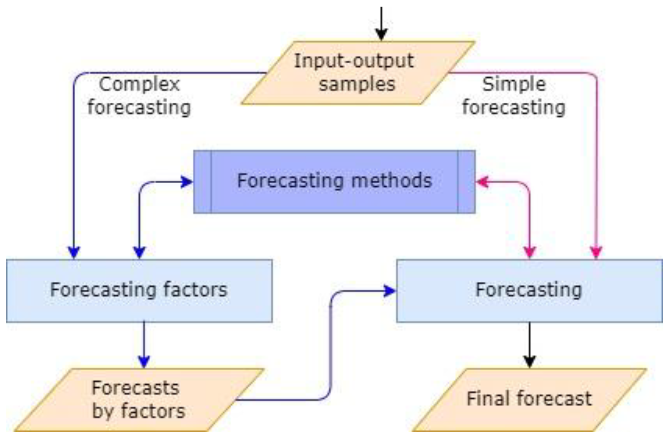
The forecasting module (
Figure 2) provides us with two different forecasting approaches:
simple forecasting—direct forecasting with known behavior of the factors, or if we consider the values of the target variable as a time series;
complex forecasting—the forecasting of the target value is based on additionally created forecast data for the individual factors.
During the process of factor forecasting, for each of the factors the most effective method was sought, which could be used repeatedly (
Figure 3). It is appropriate to forecast the individual factors in parallel and to use cloud computing to save time and resources.
The factor forecasting module receives a two-dimensional array of input data , containing the sample for in number factors, each with values. Other input parameters are the number of desired forecast values and the lower limit of the desired . For each of the factors, independent forecasts were made using the library of “prediction methods”.
The set of forecasting methods was pre-set in the software system and could be extended. The methods include a variety of time series forecast models, models based on artificial neural networks in which parameters such as the number of neurons, activation functions, learning algorithms and other artificial intelligence algorithms can be changed. Models with time series and artificial neural networks are integrated in the system so far.
Applying the forecasting methods, for each of the factors there are approximating functions with the desired efficiency .
In the process of evaluating the effectiveness, using the AE, MAE, and MSE errors, the efficiencies of the tested methods or variants of methods were compared. The most appropriate forecasting model was selected, including the method and its corresponding parameters.
The end result of the process is a set of ordered triples <factor, factor data, selected forecasting method and its corresponding parameters>, i.e., . When the data change, the same selected method can be used, or the process can be restarted to search for a new method.
3.6. Algorithm for Searching for an Optimal Artificial Neural Network
To solve a task, many different neural networks can be built, with different numbers of neurons in the hidden layer, with greater or lesser error and different result functions, which have similar behavior in the input–output samples used. An error is not always an indicator of the complexity of the neural network. The lesser number of neurons implies faster and easier learning of the neural network and, subsequently, faster work. The optimal neural network for solving a certain task has characteristics such as a minimum number of neurons and compliance with the user-specified allowable error in training, testing, and validation with the available input-output samples. Its effectiveness in newcomer input data can be evaluated at a later stage. An algorithm providing capabilities for automated construction of multiple neural networks would help choose the optimal solution.
One of our experimented approaches for creating an optimal neural network is iteration over various parameters (
Figure 4) needed to create neural networks: number of neurons in the hidden layer, activation functions (
Table 1), training algorithms (
Table 2), and number of training epochs. It successively changes the parameters for creating neural networks and examines the efficiency of the current neural network. The first neural network that meets the requirements set by the user is considered optimal. Therefore, an important part of the algorithm is how to change the iterative parameters. Since the creation and training of each neural network requires a certain amount of computer resources and time, the iterative approach is appropriate to use on single-processor machines only for tasks where finding the appropriate neural network is expected to have a relatively small number of iterations.
Finding the optimal solution faster is associated with:
Indication of parameters for changing the number of neurons. Reducing the limits of variation in the number of neurons will reduce the total number of iterations in the algorithm and therefore will accelerate the achievement of the final result—the creation of an optimal neural network. In some cases, the expected number of neurons can be justified mathematically [
40,
41].
Arrangement of the used training methods and activation functions. Different activation functions are suitable for different tasks. To solve problems requiring the application of mathematical logic, we included the hard-limit transfer function and its variant—the Symmetric hard-limit transfer function. These functions provide an interrupted binary signal along the axon of neurons and are suitable in case there is a need to solve problems requiring binary logical thinking. On the other hand, to forecast the future development of continuous processes, we used a large number of efficient and convenient transfer functions. Priority in the order of use is given to those with a sigmoid character such as hyperbolic tangent sigmoid transfer function and log-sigmoid transfer function, useful in a very wide range of problems [
42].
Necessity to change the number of learning epochs. Sometimes, to reach the optimal neural network it is only necessary to change the number of training epochs. Increasing the iterations slows down the neural network learning process, but often even a slight change in this parameter leads to a surprising overcoming of a small plateau of neural network errors and leads to a sharp improvement in the final approximation.
The iterative algorithm for automated construction of artificial neural networks (
Figure 5) has the following main steps:
- (1)
Preparation of input data:
Tensor data—input data for the factors, which are usually in the form of a one-dimensional——or two-dimensional array—.
Number of forecasted results——which is 1 for single-point forecasts or a larger integer for multi-step forecasts.
Desired efficiency——of the trained neural network.
- (2)
Preparation of the parameters on which iteration is performed:
List of training methods
, where
varies from
1 to the number of methods (
Table 2). Depending on the task, to achieve the desired result faster, it is possible to arrange the methods in the list according to the expected efficiency, and some of them may even be excluded if they are considered inappropriate.
List of activation functions
, where
varies from
1 to the number of functions (
Table 1). Here, too, the functions can be arranged at the discretion of the appropriateness of their use in the specific task.
Minimal and maximal number of neurons— u , as well as a step by which neurons change—. The current number of neurons we denote by . For more elementary tasks, the number of neurons may start from 1 () and the step by which their number increases is also 1. The maximum number limits the possible iterations related to the number of neurons.
The epochs change from to with a step . Values we have experimented with are , where usually 3–4 iterations are enough to assess whether the change of epochs affects the efficiency of the trained neural network.
By iterating over the number of neurons, training methods and activation functions, a neural network with their current values is created—the ordered triple and the input data. The nesting of the loops for the specific task is a matter of judgment, which determines the sequence of the parameters change. In the experiments, we chose to increase the number of neurons in the outermost loop, as we wanted to find a neural network with the lowest number of neurons. Training methods and activation functions change in inner loops.
- (3)
After the creation of the current neural network, it is trained, tested, and validated.
- (4)
The desired efficiency is compared to the efficiency of the current neural network, and then:
If the neural network meets the condition, its data is saved and the task is completed;
Otherwise, attempts are made to increase the efficiency of the neural network by increasing the number of learning epochs. The information about the most efficient neural network found (with the smallest error) is saved, and it can be current or obtained in a previous iteration.
- (5)
The end result of the algorithm is a trained neural network having the closest possible to the specified efficiency, as well as parameters for its architecture and training—efficiency, number of neurons n, training method lm, activation function af, and epochs ep.
The use of the “brute force” method, by traversing all possible values of the iterative parameters and finding the neural network with the optimal ratio “number of neurons—efficiency” is not the most rational approach. Tracking changes in the specified ratio can lead to the creation of heuristic variants of the algorithm by automated changing of the order of change of the iterative parameters.
The availability of sufficient computing power predisposes to the use of different parallel algorithms for such automated search for an optimal neural network (
Figure 5) in which, for example, all combinations of training methods and activation functions can be started in parallel processes—(
, where
and
are changed from
1 to the corresponding number of training methods and activation functions. After the completion of the individual processes, the efficiencies of all neural networks created during their implementation are compared and the most appropriate one is selected.
4. Results and Discussion
A prototype was developed for approbation of the presented model. The program MatLab was used, with which the described basic modules and functionalities were implemented. The prototype was tested to solve prognostic tasks in the field of energy.
4.1. Setup of the Experiment
The problem of forecasting the demand and respectively—the consumption of electricity is extremely important for the planning and management of the national energy system of every country. Accurate forecasting of probable electrical loads is an important prerequisite for effective planning of production capacity, proper maintenance of the transmission and distribution network, planning of future exports or imports of electricity, the behavior and direction of energy flows both in the country and in related international networks.
The developed prototype was used to solve three tasks for forecasting electricity consumption in the National Power System of Bulgaria. The targets subject to forecasting were:
- (1)
Total final consumption in the national power system;
- (2)
Electricity consumption in the industry, the public sector, and services;
- (3)
Electricity consumption in households.
The forecasts were made by taking into account their dependencies on the following socio-economic factors:
- (1)
Gross domestic product (GDP);
- (2)
Energy intensity (EI);
- (3)
Population;
- (4)
Income of the population;
- (5)
Energy efficiency;
- (6)
Price of electricity.
These factors have been identified as significant in studies carried out by the Bulgarian Academy of Sciences (BAS) and Risk Management Lab [
10,
11]. A subsequent step would be to build a module for the automated study of correlations between the factors with the aim of minimizing their number and optimizing post-processing.
In order to forecast the target values for a specific year, we first made forecasts for the factors for the respective year.
In the process of work, data from official sources such as the National Statistical Institute [
42], Information System INFOSTAT [
43], Electricity System Operator [
44], The World Bank Group [
45], and Eurostat [
46] were used. All available data on factors and target values for 17 years were used for the study.
The factor forecasting module uses different models of the time series trend. A substructure involving the use of neural networks to predict these factors provides for the possibility of further processing of the input data. Some of the data are submitted to the neural networks normalized, which is implemented by multiplying them by a specific coefficient. This reduces the radius vector of the input data and facilitates the training of this type of artificial intelligence. The general scheme showing the joint operation of the modules is shown in
Figure 6:
- (1)
Modules for factor forecasting, respectively through time series and neural networks;
- (2)
Error estimation module (mediator module) for the various methods and parameters;
- (3)
Consumption forecasting module.
4.2. Single-Point Forecasts for the Factors
The use of the prototype for forecasting electricity consumption in single-point (annual) factor forecasting showed different results for the effectiveness of different types of trends in time series (
Figure 6).
When forecasting GDP, population, and average annual income, maximum efficiency was achieved with a linear trend of the time series. The forecasting of the energy intensity, the price of the electricity for the household, and the price of the electricity for the industry achieved good results respectively in logarithmic, quadratic, and hyperbolic trends of the time series. Models for the most efficient neural networks, forecasting the same factors, are presented in
Figure 7.
During neural network training, all factors were considered as functions of time in order to enable the comparison of the results of forecasting in time series. The type of training that proved to be most effective for current tasks is the Lavenberg–Marquardt algorithm. The most appropriate activation function of neurons in the hidden layers for Energy intensity of the economy neural network is the logarithmic sigmoid function:
and for every other it is the hyperbolic tangent:
The activation function of the output neuron in all neural networks is linear:
The comparative analysis between the efficiency of the found neural networks in a one-year forecast and the type of trend in time series, leading to minimal error, is presented in
Figure 8.
The use of the presented prototype with time series and artificial neural networks showed a significant advantage in favor of neural networks in the case of forecasting GDP, population, and average annual income. In the other three cases, single-point forecast of energy intensity, price of electricity for households and its price for the economy sector, the module for comparison of errors showed some advantage in the efficiency of time series. In these cases, the type of trend was logarithmic, quadratic, and hyperbolic, respectively. Based on them, forecasts were made for the development of the values of the factors presented in
Table 3.
4.3. Multifactor Single-Point Forecasts of Target Values
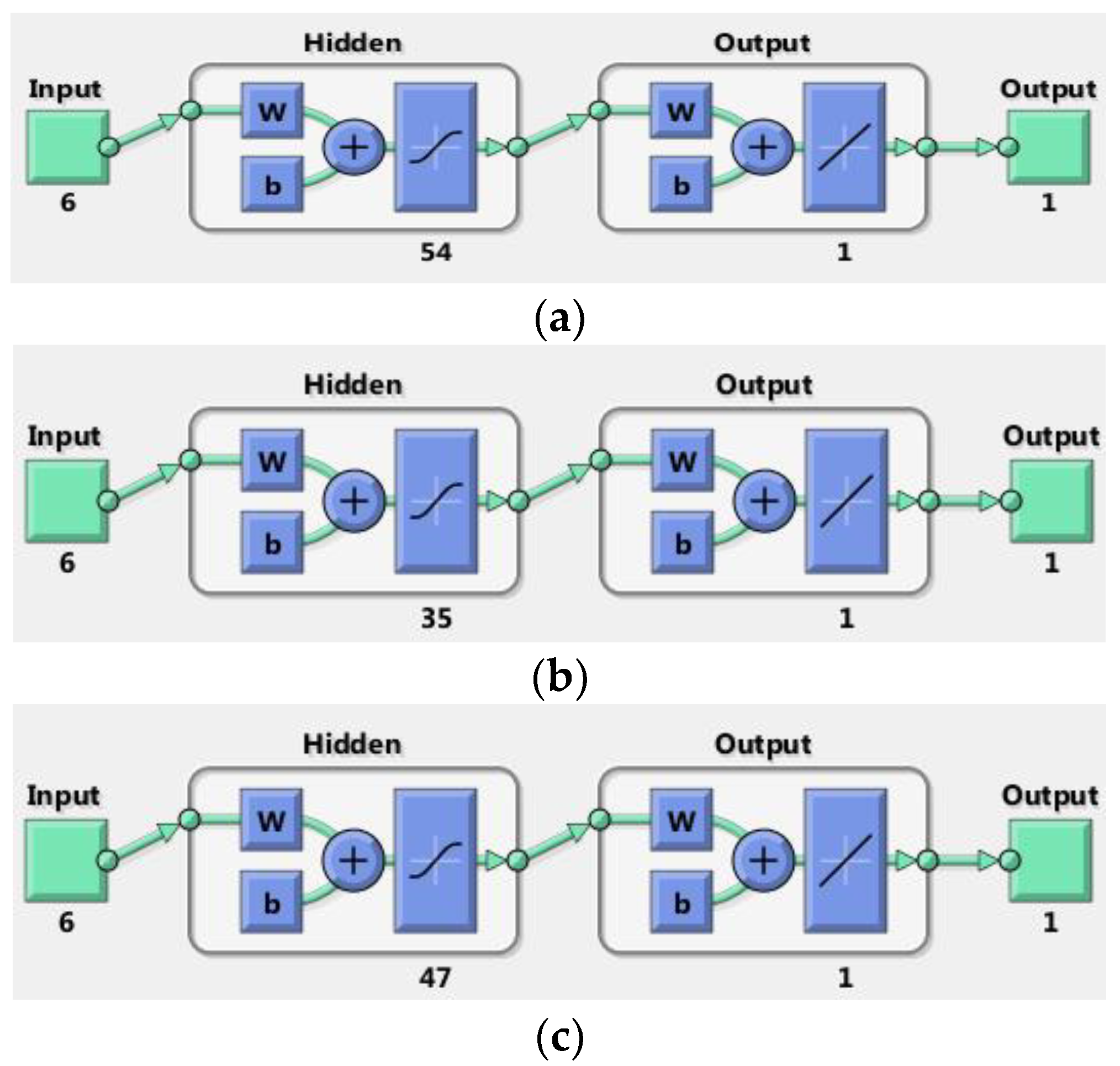
In the second part of the conducted experiments, the influence of the considered factors on the target values in the National Power System of Bulgaria was studied. Appropriate optimal neural structures were created for their forecast (
Figure 9):
- (1)
Total final consumption in the National Power System—the neural network named Net_Nees, with 54 neurons in the hidden layer;
- (2)
Electricity consumption in industry, public sector and services—Net_Industry neural network with 35 neurons in the hidden layer;
- (3)
Electricity consumption on households—Net_Household neural network with 47 neurons in the hidden layer.
Activation functions of all neural networks found by the software system were hyperbolic tangent, and of the output neuron, linear.
The deviations of the forecast results from the actual data for single-point forecasts (for one-year consumption) were relatively small (
Table 4) as the largest deviations in forecasting consumption in the industry are about 41 thousand tons of oil (toe) equivalent, i.e., about 1.525%. The deviation in forecasting consumption in the entire energy system was 0.0739%, and household consumption was 0.0302%.
Considering complex values as time series did not provide good results. The errors obtained with the best approximations of time series were many times worse than the corresponding neural networks (
Table 5).
The analysis of the weights of the neural networks can show us the influence of the individual factors on the predicted value of the target variable.
Let us denote by
the weights by which the
-th factor is transmitted to the neuron
from the hidden layer of the already trained neural network, as
. We choose the value as a criterion for the significance of factor
:
where
r is the number of neurons in the hidden layer of the neural network.
The study showed that the largest impact on the total electricity consumption in the national network belongs to the gross domestic product of the country with , and the least to the average annual income per capita with . For consumption in the industry sector, things are similar. The most significant factor was GDP with , and the one with the least importance was the price of electricity for the household—. The most important factors in the energy consumption of households are population ( and average annual income—.
4.4. Multi-Step Forecasts
Using the created neural structures for factor forecasting, we created forecasts for a period of 7 years. Their accuracy can be determined over time (
Table 6). Similarly, we created 7-year forecasts for the studied multifactorial values (
Table 7). The forecast results showed that household electricity consumption, as well as total final consumption, will gradually increase, while electricity consumption in industry, the public sector, and services will decrease.
5. Conclusions
Forecasting is a complex task. The availability of a wide variety of mathematical and statistical methods, and artificial intelligence methods, combined with the pursuit of the most accurate forecasting, usually requires a lot of time and effort. The use of software tools to automate some of the activities greatly simplifies the work.
The article proposed a model for multifactor forecasting which automatically selects the best method for forecasting significant factors and then uses the data predicted by them to create a complex multifactor forecast. The developed model was successfully experimented with to make multiple forecasts for the energy consumption of households, industry, and total consumption—for a one-year and a seven-year period. By automating the forecasting process in an indicative way, we made it easier to make predictions with fewer errors than previously.
The presented model has wide applications in various subject areas. It can be used for air quality forecasting, demographic forecasting, forecasting in industry, etc.
In the future, the system can be expanded in several directions. An important part of its development is the integration of additional forecasting methods. The development of a module to evaluate the correlation between the individual factors and the target variable would also help to optimize the forecasting process. Automated generation of graphics and documentation for each step in the overall forecasting process would be beneficial to the end user of the system.


