
Green Credit Financing and Emission Reduction Decisions in a Retailer-Dominated Supply Chain with Capital Constraint

Abstract
:1. Introduction
- (1)
- Is the GCF at a discounted interest rate conducive to driving the capital-constrained supplier to implement low-carbon innovation and increase his profit?
- (2)
- Is the retailer willing to provide partial prepayment to alleviate the supplier’s financial pressure?
- (3)
- Can mixed financing with a price-discount contract coordinate the supply chain?
2. Literature Review
2.1. Operations Management under a Low-Carbon Supply Chain
2.2. Research on Supply Chain Finance
2.3. Research on Green Finance
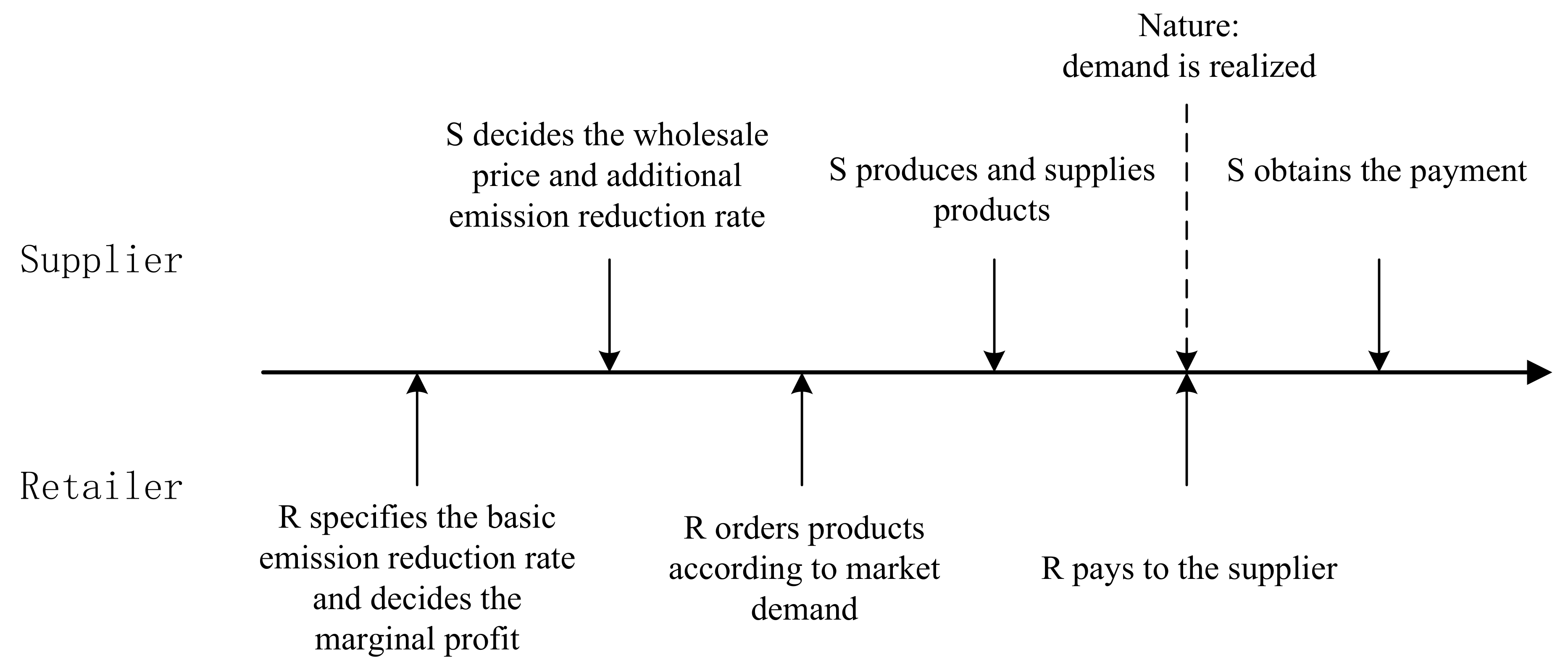
3. Model
3.1. Model a: Benchmark Model
3.2. Model b: Mixed Financing without Price-Discount Contract
3.3. Model c: Mixed Financing with Price-Discount Contract
4. Numerical Analysis
4.1. Impact of on the Profits
4.2. Impact of on the Profits
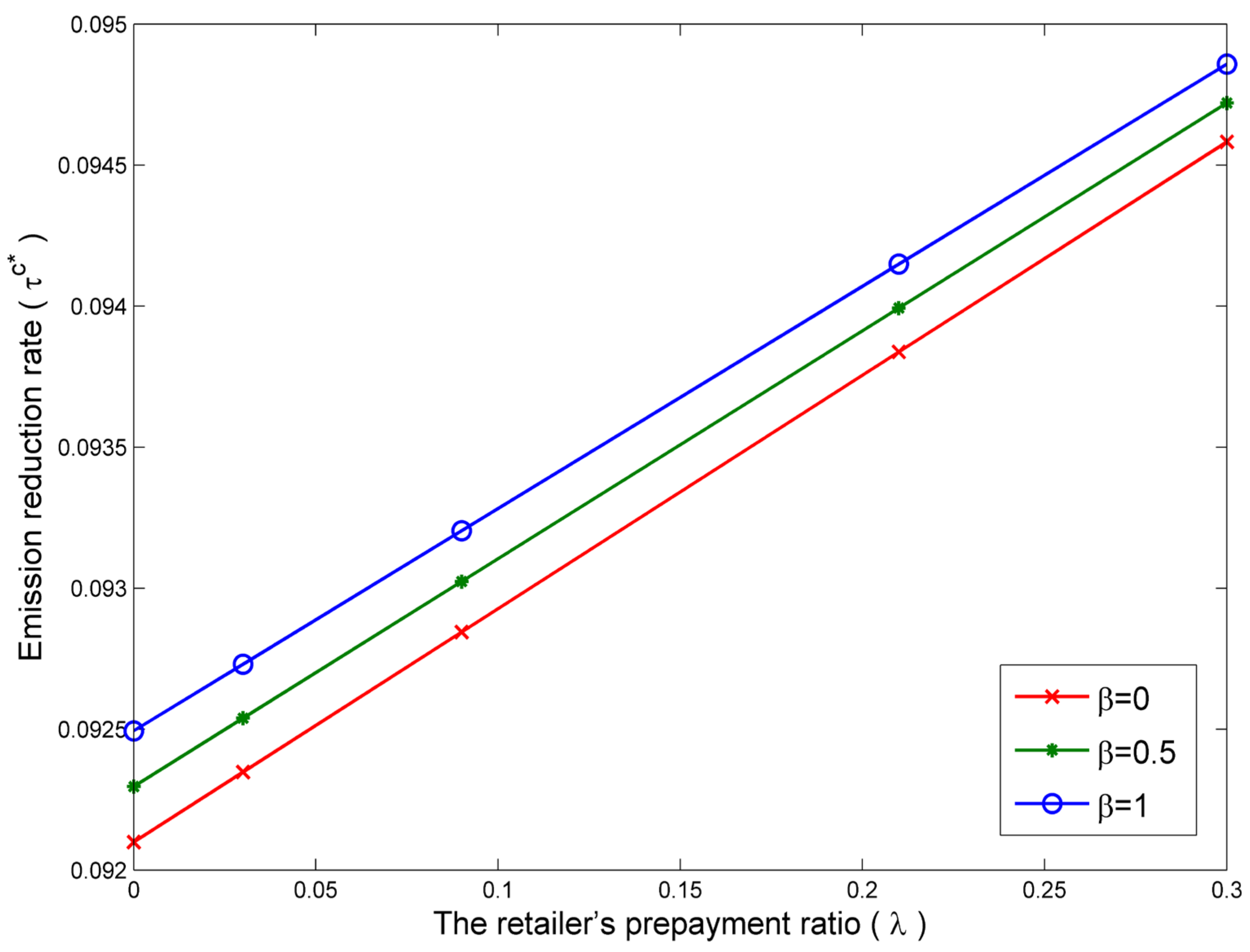
4.3. Impact of and on the Emission Reduction Rate and Profits
4.4. Impact of , , and on the Emission Reduction Rate and Profits
5. Managerial Insights
6. Conclusions
Author Contributions
Funding
Institutional Review Board Statement
Informed Consent Statement
Data Availability Statement
Conflicts of Interest
Appendix A
Appendix A.1. Proof of Lemma 1
Appendix A.2. Proof of Lemma 2
Appendix A.3. Proof of Proposition 1
Appendix A.4. Proof of Proposition 2
Appendix A.5. Proof of Proposition 3
Appendix A.6. Proof of Proposition 4
Appendix A.7. Proof of Proposition 5
Appendix A.8. Proof of Lemma 3
Appendix A.9. Proof of Corollary 1
Appendix A.10. Threshold Values
References
- Xia, X.Q.; Li, C.Y.; Zhu, Q.H. Game analysis for the impact of carbon trading on low-carbon supply chain. J. Clean. Prod. 2020, 276, 123220. [Google Scholar] [CrossRef]
- Ma, J.; Wang, Z. Optimal pricing and complex analysis for low-carbon apparel supply chains. Appl. Math. Model. 2022, 111, 610–629. [Google Scholar] [CrossRef]
- Vieira, L.C.; Longo, M.; Mura, M. Are the European manufacturing and energy sectors on track for achieving net-zero emissions in 2050? An empirical analysis. Energy Policy 2021, 156, 112464. [Google Scholar] [CrossRef]
- Xue, Q.T.; Feng, S.X.; Chen, K.R.; Li, M.C. Impact of digital finance on regional carbon emissions: An empirical study of sustainable development in China. Sustainability 2022, 14, 8340. [Google Scholar] [CrossRef]
- An, S.; Li, B.; Song, D.; Chen, X. Green credit financing versus trade credit financing in a supply chain with carbon emission limits. Eur. J. Oper. Res. 2021, 292, 125–142. [Google Scholar] [CrossRef]
- Luo, Y.; Wei, Q.; Ling, Q.H.; Huo, B.F. Optimal decision in a green supply chain: Bank financing or supplier financing. J. Clean. Prod. 2020, 271, 122090. [Google Scholar] [CrossRef]
- Fang, L.; Xu, S. Financing equilibrium in a green supply chain with capital constraint. Comput. Ind. Eng. 2020, 143, 106390. [Google Scholar] [CrossRef]
- Cao, E.; Yu, M. Trade credit financing and coordination for an emission-dependent supply chain. Comput. Ind. Eng. 2018, 119, 50–62. [Google Scholar] [CrossRef]
- Jing, B.; Chen, X.; Cai, G.G. Equilibrium financing in a distribution channel with capital constraint. Prod. Oper. Manag. 2012, 21, 1090–1101. [Google Scholar] [CrossRef]
- Walker, H.; Preuss, L. Fostering sustainability through sourcing from small businesses: Public sector perspectives. J. Clean. Prod. 2008, 16, 1600–1609. [Google Scholar] [CrossRef]
- Tolliver, C.; Keeleyab, A.R.; Managi, S. Drivers of green bond market growth: The importance of Nationally Determined Contributions to the Paris Agreement and implications for sustainability. J. Clean. Prod. 2020, 224, 118643. [Google Scholar] [CrossRef]
- Wang, C.; Wang, W.; Huang, R. Supply chain enterprise operations and government carbon tax decisions considering carbon emissions. J. Clean. Prod. 2017, 152, 271–280. [Google Scholar] [CrossRef]
- Hong, Z.; Dai, W.; Luh, H.; Yang, C. Optimal configuration of a green product supply chain with guaranteed service time and emission constraints. Eur. J. Oper. Res. 2018, 266, 663–677. [Google Scholar] [CrossRef]
- Li, N.; Deng, M.; Mou, H.; Tang, D.; Fang, Z.; Zhou, Q.; Cheng, C.; Wang, Y. Government participation in supply chain low-carbon technology R&D and green marketing strategy optimization. Sustainability 2022, 14, 8342. [Google Scholar]
- Liu, Z.; Anderson, T.D.; Cruz, J.M. Consumer environmental awareness and competition in two-stage supply chains. Eur. J. Oper. Res. 2012, 218, 602–613. [Google Scholar] [CrossRef]
- Zhang, L.H.; Wang, J.G.; You, J.X. Consumer environmental awareness and channel coordination with two substitutable products. Eur. J. Oper. Res. 2015, 241, 63–73. [Google Scholar] [CrossRef]
- Sun, L.; Cao, X.; Alharthi, M.; Zhang, J.; Taghizadeh-Hesary, F.; Mohsin, M. Carbon emission transfer strategies in supply chain with lag time of emission reduction technologies and low-carbon preference of consumers. J. Clean. Prod. 2020, 264, 121664. [Google Scholar] [CrossRef]
- Ghosh, S.K.; Seikh, M.R.; Chakrabortty, M. Analyzing a stochastic dual-channel supply chain under consumers’ low carbon preferences and cap-and-trade regulation. Comput. Ind. Eng. 2020, 149, 106765. [Google Scholar] [CrossRef]
- Wang, Q.P.; Zhao, D.Z.; He, L.F. Contracting emission reduction for supply chains considering market low-carbon preference. J. Clean. Prod. 2016, 120, 72–84. [Google Scholar] [CrossRef]
- Wang, Y.Y.; Yu, Z.Q.; Jin, M.Z.; Mao, J.F. Decisions and coordination of retailer-led low-carbon supply chain under altruistic preference. Eur. J. Oper. Res. 2021, 293, 910–925. [Google Scholar] [CrossRef]
- Ji, J.N.; Huang, J.S. Research on single/cooperative emission reduction strategy under different power structures. Environ. Sci. Pollut. Res. 2022, 29, 55213–55234. [Google Scholar] [CrossRef] [PubMed]
- Moretto, A.; Grassi, L.; Caniato, F.; Giorgino, M.; Ronchi, S. Supply chain finance: From traditional to supply chain credit rating. J. Purch. Supply Manag. 2019, 25, 197–217. [Google Scholar] [CrossRef]
- Tsai, K.S. Financing Small and Medium Enterprises in China: Recent Trends and Prospects Beyond Shadow Banking; HKUST IEMS Working Paper Series 2015-24; HKUST Institute for Emerging Market Studies: Hongkong, China, 2015. [Google Scholar]
- Lee, H.H.; Zhou, J.; Wang, J.Q. Trade credit financing under competition and its impact on firm performance in supply chains. Manuf. Serv. Oper. Manag. 2017, 20, 36–52. [Google Scholar] [CrossRef]
- Lee, C.H.; Rhee, B.D. Trade credit for supply chain coordination. Eur. J. Oper. Res. 2011, 214, 136–146. [Google Scholar] [CrossRef]
- Gao, G.X.; Fan, Z.P.; Fang, X.; Lim, Y.F. Optimal Stackelberg strategies for financing a supply chain through online peer-to-peer lending. Eur. J. Oper. Res. 2018, 267, 585–597. [Google Scholar] [CrossRef]
- Wang, C.F.; Fan, X.J.; Yin, Z. Financing online retailers: Bank vs. electronic business platform, equilibrium, and coordinating strategy. Eur. J. Oper. Res. 2019, 276, 343–356. [Google Scholar] [CrossRef]
- Aljazzar, S.M.; Gurtu, A.; Jaber, M.Y. Delay-in-payments-a strategy to reduce carbon emissions from supply chains. J. Clean. Prod. 2018, 170, 636–644. [Google Scholar] [CrossRef]
- Zhen, X.P.; Shi, D.; Li, Y.J.; Zhang, C. Manufacturer’s financing strategy in a dual-channel supply chain: Third-party platform, bank, and retailer credit financing. Transp. Res. Part E Logist. Transp. Rev. 2020, 133, 101820. [Google Scholar] [CrossRef]
- Tang, R.H.; Yang, L. Financing strategy in fresh product supply chains under e-commerce environment. Electron. Commer. Res. Appl. 2020, 39, 100911. [Google Scholar] [CrossRef]
- Kouvelis, P.; Zhao, W. The newsvendor problem and price-only contract when bankruptcy costs exist. Prod. Oper. Manag. 2011, 20, 921–936. [Google Scholar] [CrossRef]
- Yan, N.; He, X.; Liu, Y. Financing the capital-constrained supply chain with loss aversion: Supplier finance vs. supplier investment. Omega 2019, 88, 162–178. [Google Scholar] [CrossRef]
- Tunca, T.I.; Zhu, W.M. Buyer intermediation in supplier finance. Manag. Sci. 2018, 64, 5461–5959. [Google Scholar] [CrossRef]
- Deng, S.M.; Gu, C.C.; Cai, G.S.; Li, Y.H. Financing multiple heterogeneous suppliers in assembly systems: Buyer finance vs. bank finance. Manuf. Serv. Oper. Manag. 2018, 20, 53–69. [Google Scholar] [CrossRef]
- Reindorp, M.; Tanrisever, F.; Lange, A. Purchase order financing: Credit, commitment, and supply chain consequences. Oper. Res. 2018, 66, 1287–1303. [Google Scholar] [CrossRef]
- Devalkar, S.K.; Krishnan, H. The impact of working capital financing costs on the efficiency of trade credit. Prod. Oper. Manag. 2019, 28, 878–889. [Google Scholar] [CrossRef]
- Li, X.; Lu, T.; Lin, J. Bank interest margin and green lending policy under sunflower management. Sustainability 2022, 14, 8643. [Google Scholar] [CrossRef]
- Yang, H.X.; Miao, L.; Zhao, C. The credit strategy of a green supply chain based on capital constraints. J. Clean. Prod. 2019, 224, 930–939. [Google Scholar] [CrossRef]
- Kang, K.; Zhao, Y.; Zhang, J.; Qiang, C. Evolutionary game theoretic analysis on low-carbon strategy for supply chain enterprises. J. Clean. Prod. 2019, 230, 981–994. [Google Scholar] [CrossRef]
- Cao, E.; Yu, M. The bright side of carbon emission permits on supply chain financing and performance. Omega 2019, 88, 24–39. [Google Scholar] [CrossRef]
- Wu, D.D.; Yang, L.; Olson, D.L. Green supply chain management under capital constraint. Int. J. Prod. Econ. 2019, 215, 3–10. [Google Scholar]
- Zhang, Y.M.; Chen, W. Optimal production and financing portfolio strategies for a capital-constrained closed-loop supply chain with OEM remanufacturing. J. Clean. Prod. 2021, 279, 123467. [Google Scholar] [CrossRef]
- Qin, J.J.; Zhao, Y.H.; Xia, L.J. Carbon emission reduction with capital constraint under greening financing and cost sharing contract. Int. J. Environ. Res. Public Health 2018, 15, 750. [Google Scholar] [CrossRef] [PubMed] [Green Version]
- Tang, R.H.; Yang, L. Impacts of financing mechanism and power structure on supply chains under cap-and-trade regulation. Transp. Res. Part E Logist. Transp. Rev. 2020, 139, 101957. [Google Scholar] [CrossRef]
- Li, Q.; Long, R.; Chen, H. Empirical study of the willingness of consumers to purchase low carbon products by considering carbon labels: A case study. J. Clean. Prod. 2017, 161, 1237–1250. [Google Scholar] [CrossRef]
- Wong, E.Y.C.; Chan, F.F.Y.; So, S. Explaining consumer choice of low carbon footprint goods using the behavioral spillover effect in German-speaking countries. J. Clean. Prod. 2020, 242, 118404. [Google Scholar] [CrossRef]
- Savaskan, R.C.; Wassenhove, L.N.V. Reverse channel design: The case of competing retailers. Manag. Sci. 2006, 52, 1–14. [Google Scholar] [CrossRef]
- Subramanian, R.; Gupta, S.; Talbot, B. Compliance strategies under permits for emissions. Prod. Oper. Manag. 2007, 16, 763–779. [Google Scholar] [CrossRef]
- Swami, S.; Shah, J. Channel coordination in green supply chain management. J. Oper. Res. Soc. 2013, 64, 336–351. [Google Scholar] [CrossRef]
- Luo, Z.; Chen, X.; Wang, X. The role of co-opetition in low carbon manufacturing. Eur. J. Oper. Res. 2016, 253, 392–403. [Google Scholar] [CrossRef]
- Xu, S.; Fang, L. Partial credit guarantee and trade credit in an emission-dependent supply chain with capital constraint. Transp. Res. Part E Logist. Transp. Rev. 2020, 135, 101859. [Google Scholar] [CrossRef]
- Ji, J.N.; Zhang, Z.Y.; Yang, L. Carbon emission reduction decisions in the retail-/dual-channel supply chain with consumers’ preference. J. Clean. Prod. 2017, 141, 852–867. [Google Scholar] [CrossRef]


| Model Parameters | |
| Basic market capacity | |
| The market demand | |
| Profit function of the supplier | |
| Profit function of the retailer | |
| Unit retail price | |
| Supplier’s cost of raw materials | |
| Basic emission reduction rate, | |
| Basic loan interest rate | |
| Emission reduction investment coefficient of the supplier | |
| Retailer’s prepayment ratio for the supplier, | |
| Consumers’ price sensitivity coefficient | |
| Consumers’ low-carbon sensitivity coefficient | |
| The GCF relevant rate | |
| Discount rate of the GCF interest | |
| Price discount rate | |
| The supplier’s initial fund | |
| The supplier’s amount of loan | |
| Decision Variables | |
| Wholesale price | |
| Retailer’s marginal profit () | |
| Supplier’s additional emission reduction rate, | |
| 0 | 0 | 0.1599094537 | 100.3516681 | 200.7033362 |
| 0 | 0.5 | 0.1599094537 | 100.3516681 | 200.7033362 |
| 0 | 1 | 0.1599094537 | 100.3516681 | 200.7033362 |
| 0.05 | 0 | 0.1599094537 | 100.3516681 | 200.7033362 |
| 0.05 | 0.5 | 0.1601310971 | 100.3811621 | 200.7623242 |
| 0.05 | 1 | 0.1603532911 | 100.4106614 | 200.8213227 |
| 0.1 | 0 | 0.1599094537 | 100.3516681 | 200.7033362 |
| 0.1 | 0.5 | 0.1603532910 | 100.4106614 | 200.8213227 |
| 0.1 | 1 | 0.1607993391 | 100.4696757 | 200.9393514 |
Publisher’s Note: MDPI stays neutral with regard to jurisdictional claims in published maps and institutional affiliations. |
© 2022 by the authors. Licensee MDPI, Basel, Switzerland. This article is an open access article distributed under the terms and conditions of the Creative Commons Attribution (CC BY) license (https://creativecommons.org/licenses/by/4.0/).
Share and Cite
Ji, J.; Tang, D.; Huang, J. Green Credit Financing and Emission Reduction Decisions in a Retailer-Dominated Supply Chain with Capital Constraint. Sustainability 2022, 14, 10553. https://doi.org/10.3390/su141710553
Ji J, Tang D, Huang J. Green Credit Financing and Emission Reduction Decisions in a Retailer-Dominated Supply Chain with Capital Constraint. Sustainability. 2022; 14(17):10553. https://doi.org/10.3390/su141710553
Chicago/Turabian StyleJi, Jingna, Dengli Tang, and Jiansheng Huang. 2022. "Green Credit Financing and Emission Reduction Decisions in a Retailer-Dominated Supply Chain with Capital Constraint" Sustainability 14, no. 17: 10553. https://doi.org/10.3390/su141710553