Article

Application of Machine Learning and Multivariate Statistics to Predict Uniaxial Compressive Strength and Static Young’s Modulus Using Physical Properties under Different Thermal Conditions

1
Department of Sustainable Advanced Geomechanical Engineering, Military College of Engineering, National University of Sciences and Technology, Risalpur 23200, Pakistan
2
Key Laboratory of Deep Coal Resource Mining (China University of Mining & Technology), Ministry of Education, Xuzhou 221116, China
3
Department of Mining Engineering, Balochistan University of Information Technology Engineering and Management Sciences, Quetta 87300, Pakistan
4
School of Management Science and Engineering, Anhui University of Finance and Economics, Bengbu 233030, China
5
State Key Laboratory of Mining Response and Disaster Prevention and Control in Deep Coal Mine, Anhui University of Science and Technology, Huainan 232001, China
6
School of Materials and Mineral Resources Engineering, University Sains Malaysia, Engineering Campus, Nibong Tebal 14300, Penang, Malaysia
7
Department of Mining Engineering, University of Engineering & Technology, Peshawar 25000, Pakistan
8
Department of Mining Engineering, University of Engineering and Technology, Lahore 54890, Pakistan
9
School of Resources and Safety Engineering, Central South University, Changsha 410083, China
10
Department of Mining Engineering, Karakoram International University, Gilgit 15100, Pakistan
*
Authors to whom correspondence should be addressed.
Sustainability 2022, 14(16), 9901; https://doi.org/10.3390/su14169901
Submission received: 26 May 2022 / Revised: 4 July 2022 / Accepted: 29 July 2022 / Published: 10 August 2022
(This article belongs to the Special Issue Advances in Rock Mechanics and Geotechnical Engineering)

Abstract

:
Uniaxial compressive strength (UCS) and the static Young’s modulus (Es) are fundamental parameters for the effective design of engineering structures in a rock mass environment. Determining these two parameters in the laboratory is time-consuming and costly, and the results may be inappropriate if the testing process is not properly executed. Therefore, most researchers prefer alternative methods to estimate these two parameters. This work evaluates the thermal effect on the physical, chemical, and mechanical properties of marble rock, and proposes a prediction model for UCS and ES using multi-linear regression (MLR), artificial neural networks (ANNs), random forest (RF), and k-nearest neighbor. The temperature (T), P-wave velocity (PV), porosity (η), density (ρ), and dynamic Young’s modulus (Ed) were taken as input variables for the development of predictive models based on MLR, ANN, RF, and KNN. Moreover, the performance of the developed models was evaluated using the coefficient of determination (R2) and mean square error (MSE). The thermal effect results unveiled that, with increasing temperature, the UCS, ES, PV, and density decrease while the porosity increases. Furthermore, ES and UCS prediction models have an R2 of 0.81 and 0.90 for MLR, respectively, and 0.85 and 0.95 for ANNs, respectively, while KNN and RF have given the R2 value of 0.94 and 0.97 for both ES and UCS. It is observed from the statistical analysis that P-waves and temperature show a strong correlation under the thermal effect in the prediction model of UCS and ES. Based on predictive performance, the RF model is proposed as the best model for predicting UCS and ES under thermal conditions.

1. Introduction

In recent years, investigations into and understandings of reservoir rock behaviour under differing high temperatures (T) have become imperative for the safe implementation of engineering projects [1,2,3,4,5,6,7,8]. The behaviour of rock under high temperatures is a major concern in geological sciences, underground engineering, geothermal energy exploitation, deep mining, nuclear waste disposal, engineering structures, and coal gasification. The high temperatures alter and degrade the properties of the rock mass associated with these engineering structures [9]. Granite, in particular, contains heat-producing radioactive isotopes that raise the thermal gradient and stimulate the geothermal system (EGSs) up to 350 °C [10,11,12,13]. This thermal stress dramatically affects the mechanical properties of the reservoir rock. Furthermore, different heating conditions exhibit distinct mechanical properties compared to the intact rock’s room temperature, affecting borehole stability. Therefore, it is essential to study the high thermal mechanics and their effects on the reservoir rock properties for the safe and efficient execution of the engineering project.
Previous research shows that rocks’ physical and mechanical properties are significantly affected by increasing thermal conditions due to the alteration of mineral composition and intergrain bonding [14,15,16]. Furthermore, the high temperature can cause a thermal expansion in the rock-forming mineral, inducing thermal stress in the rock resulting in the development of micro-cracks and propagating the existing cracks and length [15,17,18,19,20,21,22,23,24]. For instance, Chen et al. [25] noted that the UCS and Young’s modulus (E) of rock are decreased with the increases in temperature up to 1000 °C. Homand-Etienne and Houpert [14], and Chen, Ni, Shao, and Azzam [25], concluded from their research that the UCS of granite decreased slightly with an increase in temperature up to 400 °C, but a dramatic decline in UCS was observed when the temperature exceeded 400 °C. Peng, Rong, Cai, Yao, and Zhou [15] evaluated marble’s physical and mechanical properties and found that the UCS and E both decrease with the increase in temperature. Considering the importance of UCS and ES used as input parameters in the effective design and rock mass behaviour analysis, it is essential to evaluate these parameters under high-temperature mechanics.
It is possible determine UCS and ES by both destructive and non-destructive methods [26]. The destructive testing for both parameters is time-consuming and expensive, and the core sampling needs high precision, while the obtained results can be ambiguous [27,28]. Therefore, researchers have focused their attentions on non-destructive techniques. Several studies have been conducted using various artificial intelligent (AI) techniques to predict rock’s strength and stiffness properties [29]. In this regard, Manouchehrian et al. [26] predicted UCS using texture as input variables based on ANN and multivariate statistics. Likewise, [26,30] used porosity (η), PV, and ρ as input variables and predicted UCS and ES based on ANNs and ANFIS. Abdi, Garavand, and Sahamieh [28] proposed the ANN and MLR methods for predictive modeling of E using η in %, dry density (γd), P-wave velocity (PV), and water absorption as input variables. It was found that the prediction performance of ANN is better than MLR. Dehghan et al. [31] predicted UCS and Es based on ANNs and MLR using PV, the point load index, the Schmidt hammer rebound number, and η as input variables. Some cutting-edge machine learning models are also adopted to predict UCS and Es. For example, Zhang et al. [32] proposed a beetle antennae search (BAS) algorithm-based RF model to accurately and effectively predict the UCS of lightweight self-compacting concrete (LWSCC). Matin et al. [33] used the RF model to select variables within several rock properties and indexes, namely porosity (η), water content, Is (50), p-wave velocity (PV), and rebound numbers (Rn), along with an effective model for the prediction of UCS and E based on the RF preferred variables. Suthar [34] appraised the potential of five modeling approaches, namely M5 model tree, RF, ANN, SVM, and Gaussian processes (GPs) for predicting the UCS of stabilized pond ashes with lime and lime sludge. Wang et al. [35] proposed an RF model to accurately predict the UCS of rocks from simple index tests. Matin et al. [33] predicted E using RF, and multivariate regression (MVR) and a generalized regression neural network (GRNN) were used for comparison. The results revealed that RF performed well compared to MVR and GRNN. Ren et al. [36] developed several ML algorithms, namely k-nearest neighbors (KNN), naive Bayes, RF, ANN, and SVM, to accurately predict rock’s UCS using ANN and SVM. Ghasemi et al. [37] evaluated the UCS and E of carbonate rocks by developing a tree-based approach. According to their findings, the applied method revealed highly accurate results. Saedi et al. [38] studied the prediction of the UCS and E of migmatite rocks by ANN, ANFIS, and multivariate regression (MVR). Shahani et al. [39] developed an XGBoost model to predict the UCS and E of intact sedimentary rock. Armaghani et al. [40] developed a hybrid model based on ANN and imperialist competitive algorithm (ICA) to predict UCS and E of granite rocks. Although, the above-discussed literature has provided useful insights into predicting the UCS and E by utilizing different machine learning approaches, there has been, to date, no significant study documented which consider the thermal effect on the physical and mechanical behaviors of rock. The temperature has a great effect on these physical and mechanical properties. Therefore, it is imperative to increase the performance of the proposed model and to explore the use of a new input variable, i.e., temperature, in predicting the UCS and Es.
This current research was carried out in the following three steps: (1) microscopic observation was performed on thin sections of various rock samples treated at different thermal conditions. (2) Secondly, the physical and mechanical properties of marble were investigated under the influence of temperature. (3) Finally, using physical and mechanical properties, such as T, PV, ρ, η, and Ed as input variables, the UCS and Es were predicted using different statistical and computational intelligence methods, including MLR, ANN, RNN, and RF. The results of this study will serve to help researchers to better understand the thermal effect on the physical and mechanical properties of rocks in a sweltering environment.

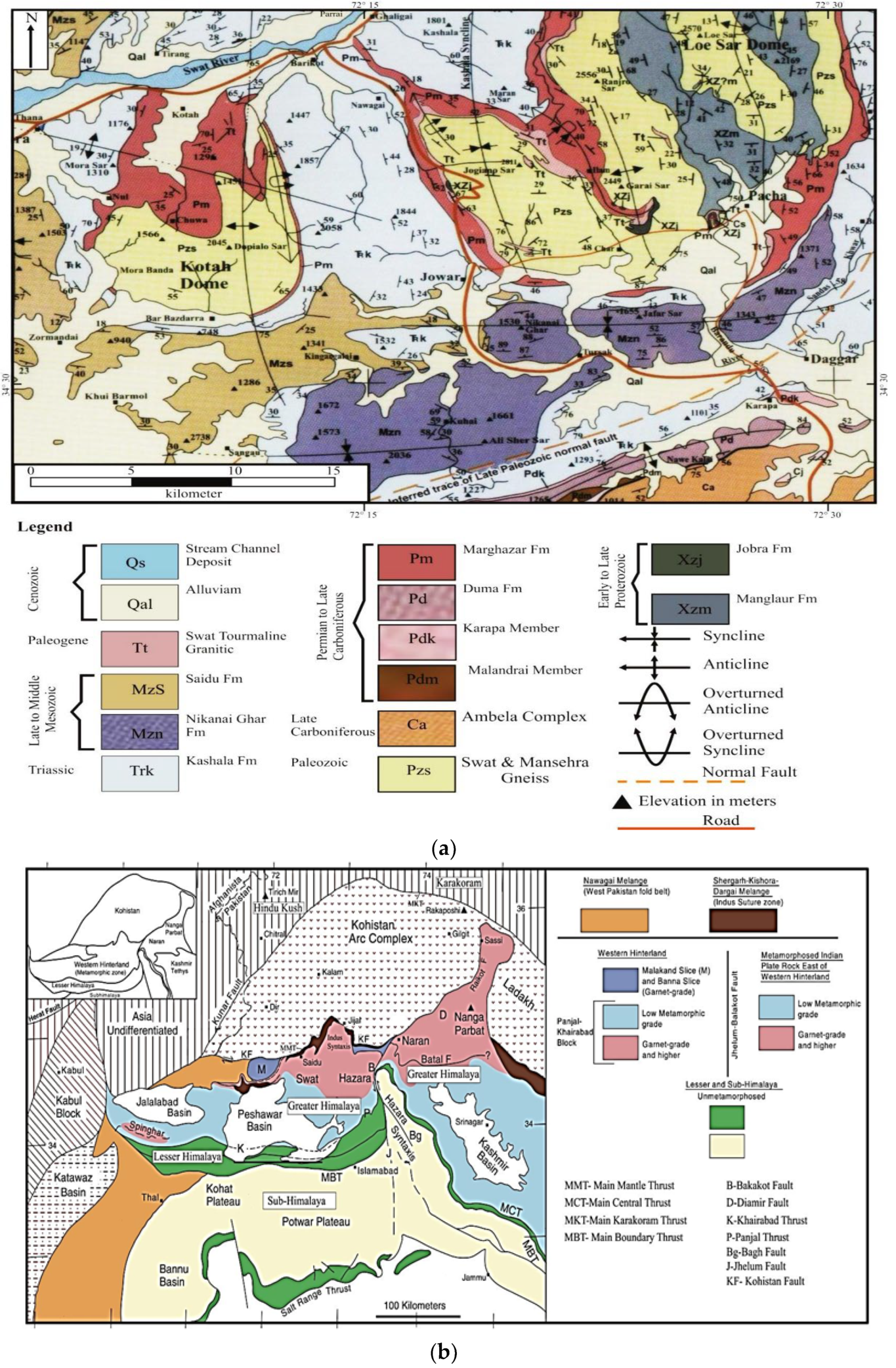
2. Regional Geological Setting

Northward subduction of the Indian Plate under the Kohistan Island Arc results in upper amphibolite, blueschist, and eclogite facies under metamorphic conditions. These high-grade metamorphic rocks form exposures from west to east in the Kotah/Loe Sar domes. At the main mantle thrust (MMT), as well as in Indus syntaxis and Nanga Parbat, there is a rapid exhumation and crustal anatexis of the Indian affinity plutonic, oceanic, and metasedimentary rocks, as shown in Figure 1a. The grade of metamorphism and deformation decrease south of the main collisional front at the MMT. The Khairabad/Panjal thrust tectonically separates the more enormous Himalayan crystalline rocks from unmetamorphosed sedimentary rocks. For this reason, dimension stones including marble, granite, granodiorites, nephrite, gabbro, quartzite, and serpentine exist between the MMT and Khairabad/Panjal Thrust presented in Figure 1a. The current research focuses on the ~ Late to Middle Mesozoic Nikanai Ghar marble of the Nikanai Ghar Formation that crops at 24 to 27 Km south of the main convergent Indian plate margin at 34.501177″ N, 72.288059″ E in the southernmost limbs of the Kotah and Loe Sar domes in the Buner district, as shown in Figure 1b. The Nikanai Ghar marble, which is spread over 700 km2 and belongs to the Alpurai Group metasediments, comprises marble, dolomite, and phyllites developed as a result of a high geothermal gradient associated with active crustal thickening and anatectic processes under the Barrovian metamorphic conditions between ca. 39 Ma and 28 Ma [41]. The total estimated marble in the district of Buner is 100 million tons. These marbles vary in color as well as in grain size [42]. The Nikani Ghar marble has a mainly fine to medium grain size. The marble individual bed thickness is 0.5–3.0 m, and the lateral extension (length) varies from 1.5–3.0 Km.
Regional geological map as presented in Figure 1a show the distribution of the greater/higher-, lesser-, and sub-Himalayan rocks. South of the convergent plate margin between the Indian plate and Kohistan Island Arc, high temperature and pressure converted limestone stratigraphic units of the greater Himalaya into marble. Indian plate basement rocks are exposed in the cores of Indus syntaxis and Nanga Parbat. The MMT separates the Indian plate from the Kohistan Island Arc. The MKT is the convergent plate boundary between the Kohistan Island Arc and Karakoram microplate [44].
A detailed geological map is presented in Figure 1b of the Lower Swat, showing the main stratigraphic and structural components of the northernmost convergent plate margin of the Indian Plate. Crustal thickening, metamorphism, and partial melting of the middle crust resulted in the Barrovian metamorphic conditions during the prograde burial of the Indian affinity rocks beneath the Kohistan Island Arc. Marble, quartzite, schist, and gneisses developed from limestone, sandstone, shale, and granite protoliths, respectively (after Hussain et al. 2004 [44]).

3. Experimental Design
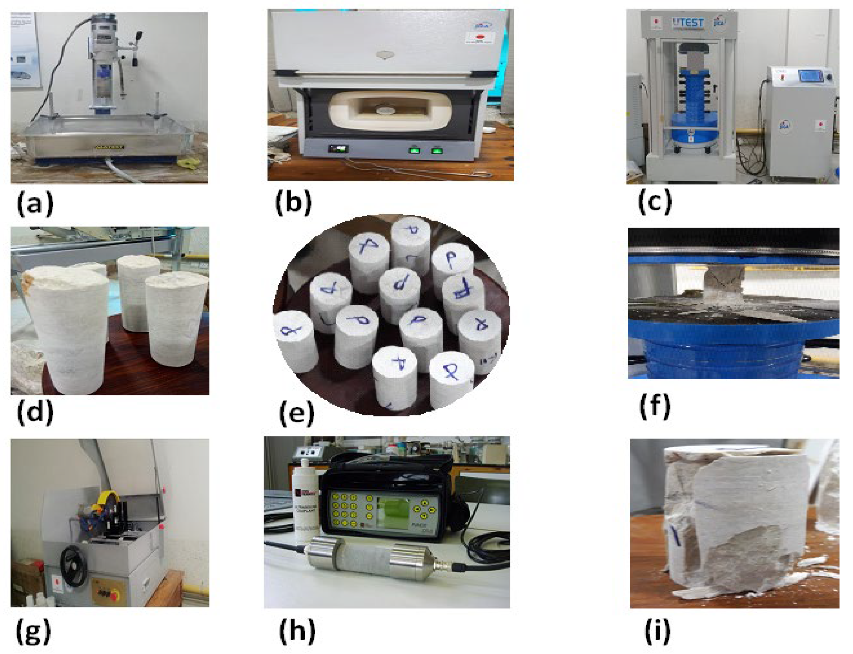
3.1. Rock Specimen

In this research, marble specimens were collected from Buner, Khyber Pakhtunkhwa, Pakistan, which has the coordinates 34.501177′′ N, 72.288059′′ E. The representative rock specimens were collected in boulder form from different points within the quarry. The cylindrical core samples (with dimensions of 54 × 108 mm) were prepared according to the International Standard of Rock Mechanics (ISRM) [45,46]. To avoid the nonparallelism between ends of the samples, the maximum allowable deviation of ±0.3 in length and ±0.5 were kept. The specimen’s ends were carefully ground and polished within 0.03 mm. The rock processing and testing scheme are shown in Figure 2.

3.2. Heating Procedure

The samples were heated in a furnace with a maximum operating temperature of 1200 °C and a power of 10 kW, as shown in Figure 2b. A total of 64 samples were heated at different predetermined temperatures in a furnace for 24 h and then cooled down gradually to room temperature. The predetermined temperatures were divided into ten groups, namely 25 °C, 200 °C, 250 °C, 300 °C, 350 °C, 400 °C, 450 °C, 500 °C, 550 °C, and 600 °C, and each group contained an average of 6 samples.

3.3. Samples Characterization

Representative samples were properly prepared, before being subjected to different types of analytical techniques for mineralogical evaluation. Thin-section study was carried out under an optical reflection microscope (Nikon Microphoto-FXA, Type 118) for mineral identification. The X’Pert PRO MPD instrument (with the specifications of Cu Kα, 40 mA current, and 40 kV voltage) was used for XRD analysis to determine the minerals; crystal size and mineral composition. A scanning electron microscope (SEM) with an energy dispersive X-ray spectrometer (SEM-EDX), with a specification of 6610LV+ OXFORD X-max, Japan, and an energy range 0–20 KV, was used for the determination of morphology and mineral microstructure element distribution in the specimen. Major oxides’ element percentage was determined in the marble sample including SiO2, Fe2O3, CaO, Al2O3, MgO, MnO, Na2O, and K2O and loss of ignition was assessed by X-ray fluorescence (XRF).

3.4. Ultrasonic Test

A portable ultrasonic nondestructive digital indicating tester (PUNDIT) was used to compute the ultrasonic parameters,0such as ultrasonic P-wave velocity. This is shown in Figure 2e. The Ed and PV were determined by an empirical relation [24].

3.5. Universal Testing Machine (UTM)

The mechanical properties of marble were determined in the laboratory by UTM, as shown in Figure 2g. The maximum capacity of machine is 250 KN. The UCS, ES, shear, and bulk modulus were determined for each predetermined temperature.

3.6. Intelligent Models

3.6.1. Multiple Linear Regression (MLR) Model

It is routine to use MLR to forecast the relationship between important parameters. It is understood that MLR is an expanded variant of basic linear regression, which is utilized in prediction modes with several predictive variables. In this study, MLR model design for UCS and ES is based on five parameters, such as T, PV, ρ, η, Ed, as shown in Table 1.
The multilinear regression result general equation is given as follows:
Y = c + b 1 X 1 + b 2 X 2 + b 3 X 3 + .......... b n X n
where, Y, c, X1 to Xn, and b1 to bn are the dependent variable, constant, independent variable, and partial regression coefficient, respectively [47,48].

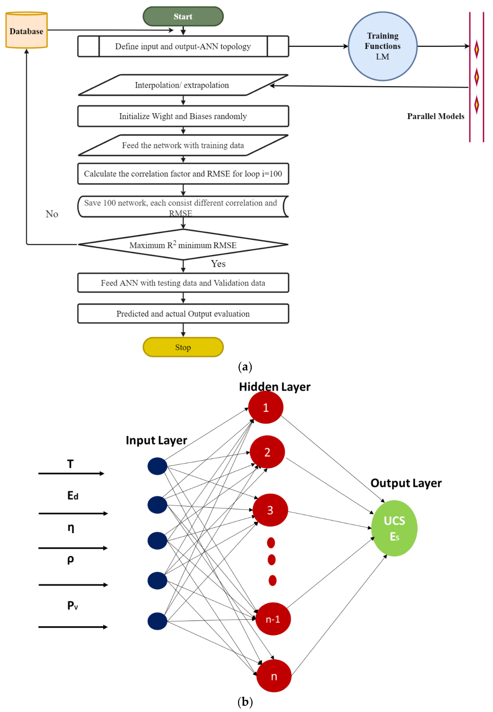
3.6.2. Artificial Neural Network (ANN) Model

An ANN plays a significant role and considered as an intelligent tool for solution of complex engineering-based problems in geotechnical engineering [49,50]. In this research, the multi-layered perception (MLP) is used. It is composed of three layers, as follows: (1) an input layer which is used to give data to the network; (2) a hidden layer which uses an algorithm and collection of features, the neurons, and the hidden layer selected on trial and error methods [51]; (3) an output layer which gives the output of the input data. Each layer contains many neurons depending on the specific application. Each layer neuron is in connection to the next successive layer and each link carries a weight [52]. Furthermore, several algorithms are used for the ANN model. Nevertheless, the most efficient is backpropagation (BP), which is used in many engineering problems due to its simple training function.
A supervised learning technique must be used throughout the training phase to ensure the accuracy and effectiveness of any classification and task in ANN. A group of examples are used in the training of the BP algorithm’s networking to connect and link the nodes and to identify the parametric function, also referred to as weight inadequate methods. In order to minimize the discrepancy between the actual output and the anticipated output, the mean square error (MSE) is repeatedly lowered. Additionally, training aids in identifying each iteration weight [53]. When training various kinds of networks, the BP method is often used. Previous research has shown that the BP method takes into account and assumes a random value. This random value is then used by the NN operation to compute output. The weight value will be adjusted in order to cut down on the margin of error, and this procedure will be repeated as many times as necessary until the minimal result is reached [54]. The model must be trained, and a wide number of scholars have provided specifics of how this might be accomplished [55,56,57].

ANN Code Compilation in MATLAB

As shown in Figure 3a, our research constructed self-generated ANN code for n numbers of networks while preserving the same training and activation function for a single loop. This code includes a loop function that may run for as many networks as the user resembling. This code’s activation function was fixed in general, but the data’s nature could be altered. In this scenario, the code was run once for 100 networks. For each network in a loop, the number of neurons increased with each successor and, thus, network1 had one neuron, network2 had two, and so forth. Different algorithms are available for ANN, but the most efficient is BP with the Levenberg–Marquardt algorithm suggested by Ullah et al. [58]. He conducted a detailed study on types of learning algorithms available for ANN. Rao and Kumar [59] concluded that the Levenberg–Marquardt (LM) is more efficient and takes less of a time epoch, while giving better results as compared to other algorithms. Therefore, LM was used in the current model for both the hidden and output layers.
The fundamental structure in this study consists of five inputs (T, PV, ρ, η, and Ed) and two outputs (UCS and ES), as illustrated in Figure 3b. The dataset consisted of 60 data points in total. The data was separated into the following three sections: training (75%), testing (15%), and validation (15%).

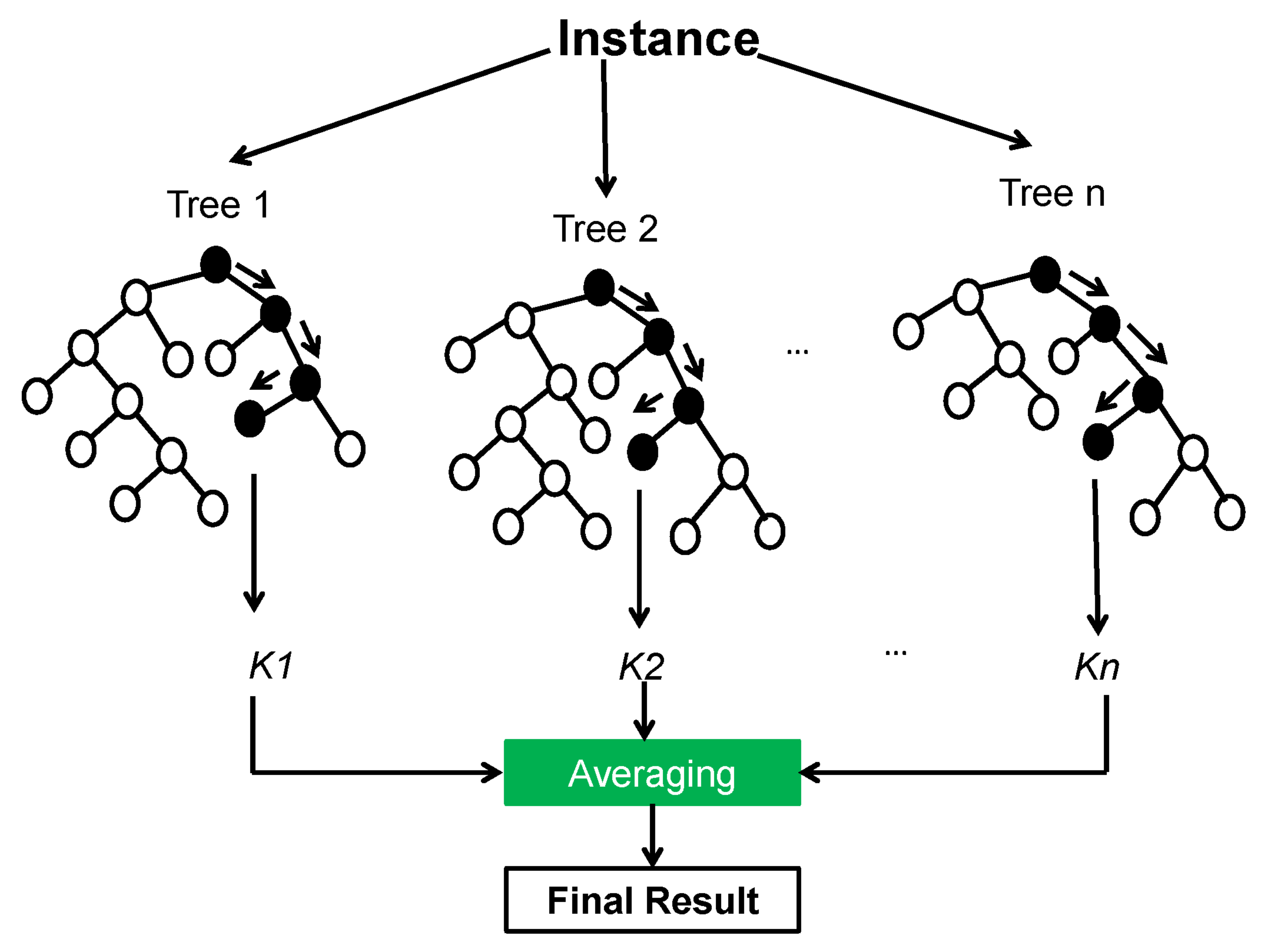
3.6.3. Random Forest Regression

The random forest regression (RFR) method was created to aid in predicting hanging wall stability, because it can explain the non-linear relationship between inputs and outputs without relying on statistical assumptions. This made it possible to pinpoint the procedure. The RFR approach is used rather often in geotechnical engineering [60], but also used for the stability of rock pillars, landslide susceptibility assessment, soil liquefaction potential, and for ground settlement prediction [58,59,60,61,62]. However, no research was documented that was associated with the use of the RFR algorithm on the prediction of the hanging wall’s stability.
Two of the most important aspects of RFR are known as the decision tree (DT) approach and the bagging methodology. Depending on the datasets, the DT approach may be used to solve problems relating to classification as well as regression. When using the DT approach, the feature space will first be segmented into sub-regions. Iterative partitioning is carried out up to the point when the termination condition is met. During the construction of a DT, three different components are produced, namely branches, internal nodes, and exterior nodes. Nodes inside the network are always linked to decision functions, which are responsible for determining which node should be visited after the current one. In a DT, the nodes that are no longer divided are referred to as the output nodes. These nodes are also sometimes called terminals or leaf nodes. Because there are problems with classification, every external node will be assigned a class label. This label will be used to classify the data that is associated with that node. When building a DT, branches are used to connect the many nodes, both internally and externally.
In spite of the fact that the DT method may be beneficial in a variety of applications, including civil engineering, Breiman [61] claims that the RFR algorithm is a more effective strategy than the DT method. This is the case despite the fact that the DT method can be used to the study of a variety of different topics. It has been shown to be more reliable than the use of a single tree in a range of data mining applications [62,63,64]. The RFR technique is a sort of ensemble learning that makes predictions based on bagging the data. Bagging is the foundation of this strategy. In the process of RFR, many of the samples collected via the bagging method are joined with those gathered through other methods to form a collection of decorrelated DTs. The results of averaging all of the DTs are employed, and this is done so that the quality of the modelling may be improved without resorting to overfitting. Figure 4 presents an overview of RF’s general architectural makeup. In this figure, the value n denotes the total number of trees, while the numbers k1, k2, etc., up to and including kn, denote the results of each individual DT.

3.6.4. k-Nearest Neighbor

The k-nearest neighbor (KNN) method is simple, powerful, and straightforward to implement [65]. In the same way that ANN and RF are used for classification and regression, so, too, is this technique. The following are some benefits associated with using this method:
  • It is straightforward to grasp and put into practice.
  • When it is employed for classification and regression, it can learn non-linear decision boundaries, and it can also invent a highly flexible choice limit by adjusting the value of K. Both of these capabilities are available when it is applied.
  • The KNN architecture does not have a step that is specifically dedicated to training.
  • Since there is only one hyperparameter, which is denoted by the letter K, adjusting the other hyperparameters is quite simple.
The essential concept behind KNN is to locate a group of “k” samples (for example, by applying distance functions) that are close in distance to unknown samples in the calibration dataset. This may be accomplished by searching for groups of samples that are similar to each other. In addition, KNN determines the class of unknown samples by calculating the average of response variables and then comparing those results to the “k” samples [66]. As a consequence of this, the value of k is critically important to the performance of the KNN [67]. For the purpose of the regression issue, the three distance function, which computes the distance between neighboring points and is presented in the following Equations (2)–(4), is utilized:
F ( e ) = i = 0 f ( x i y i ) 2
F ( m a ) = i = 0 f x i y i
F ( m a ) = i = 0 f x i y i q 1 q
where F(e) stands for the Euclidean function, F(ma) stands for the Manhattan function, F(mi) stands for the Minkowski function, xi and yi stand for the ith dimension, and q stands for the order between the points x and y.

4. Experimental Results

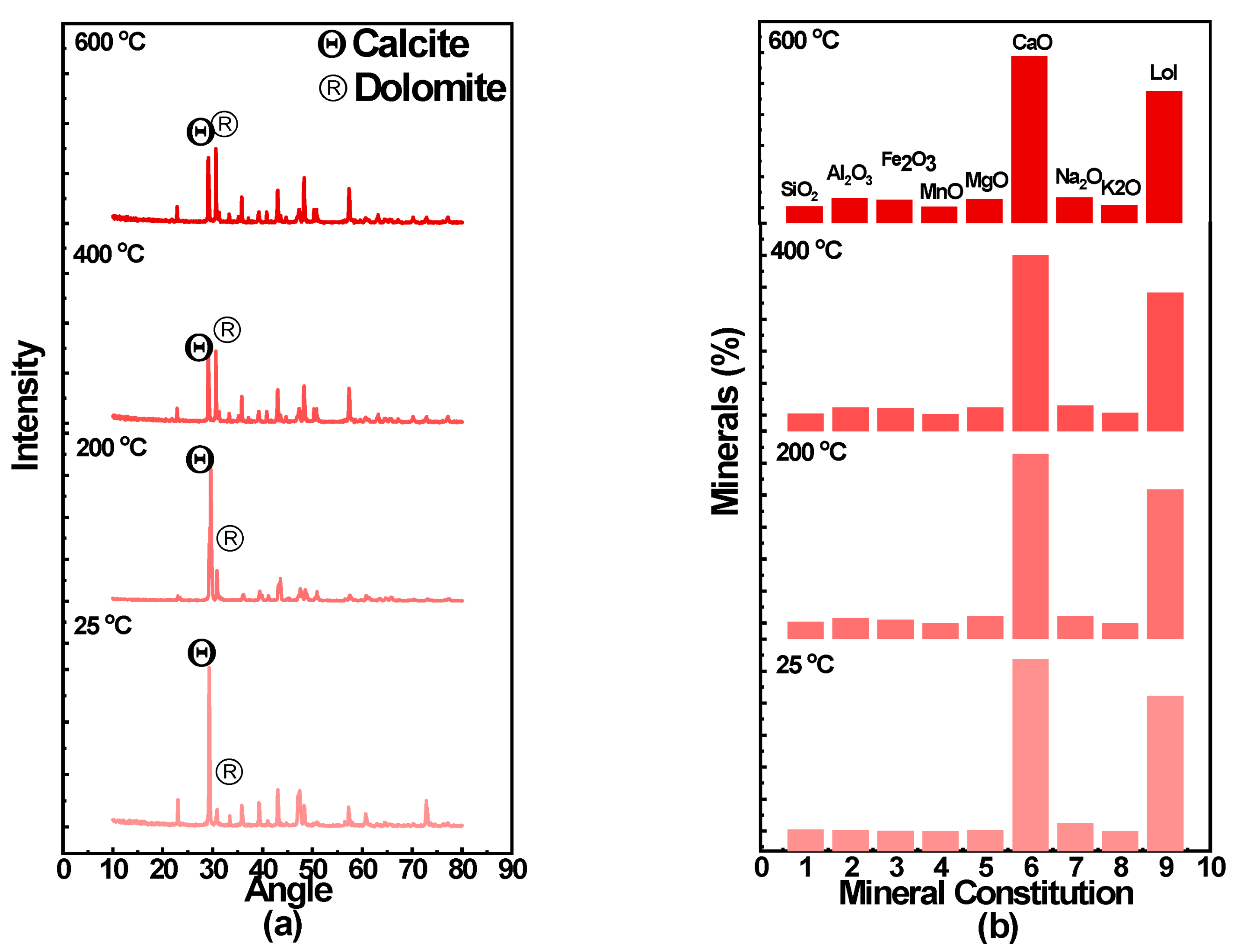
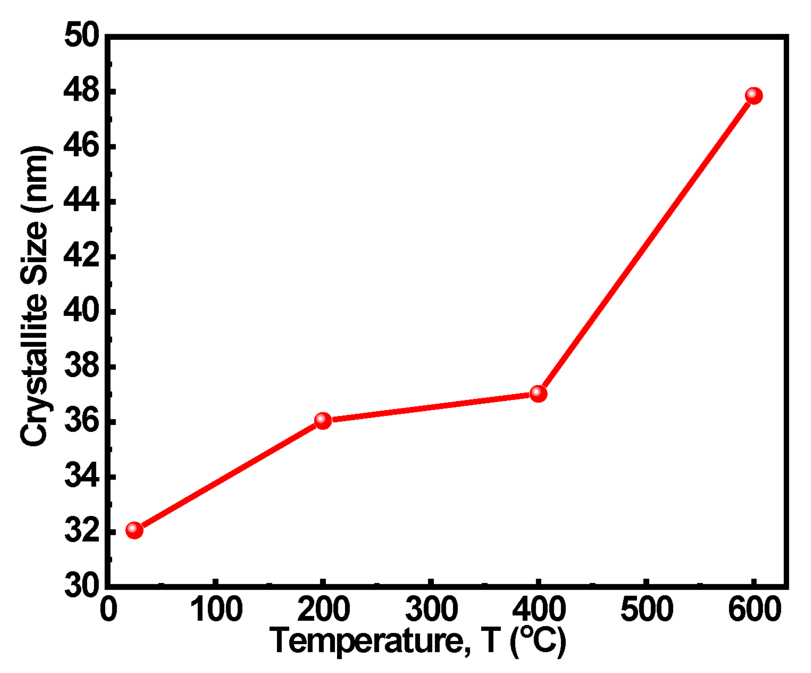
4.1. Physical Properties

The temperature significantly affects the physical properties of a rock specimen, as shown by Peng et al. [15]. As the temperature increases, and at the maximum temperature of 600 °C, the color of the sample changes from milky white to gray. It is believed that, as the temperature increases, the composition and color of the samples changes accordingly. The percentages of mineral constitution of samples at room temperature and 600 °C temperature were noted to be different. These variations are confirmed through XRD and XRF, as shown in Table 2 and Figure 5a,b. The XRD and XRF results revealed that the samples are mainly composed of calcite, dolomite, and other minerals traces, as shown in Table 2. The increase in temperature has an inverse effect on the intensity of calcite, which is confirmed from the results of the XRD and XRF, as shown in Figure 5a,b. Moreover, it is clear from Table 2 that the temperature increase does not influence the composition of marble. For each mineral, some differences in mineral composition result from the heterogeneity of the marble as described in Table 2, which is in agreement with the previous studies [68,69].
The XRD result shows that the rock is mainly composed of calcite and dolomite. The trends in Figure 5a,b show a decrease in the intensity of calcite as temperature increases. The increase in temperature also significantly increased the crystallite size that is determined using the Scherer formula. The result for different temperatures and crystallite size shows that the crystallite size increases with the increase in temperature, as presented graphically in Figure 6.

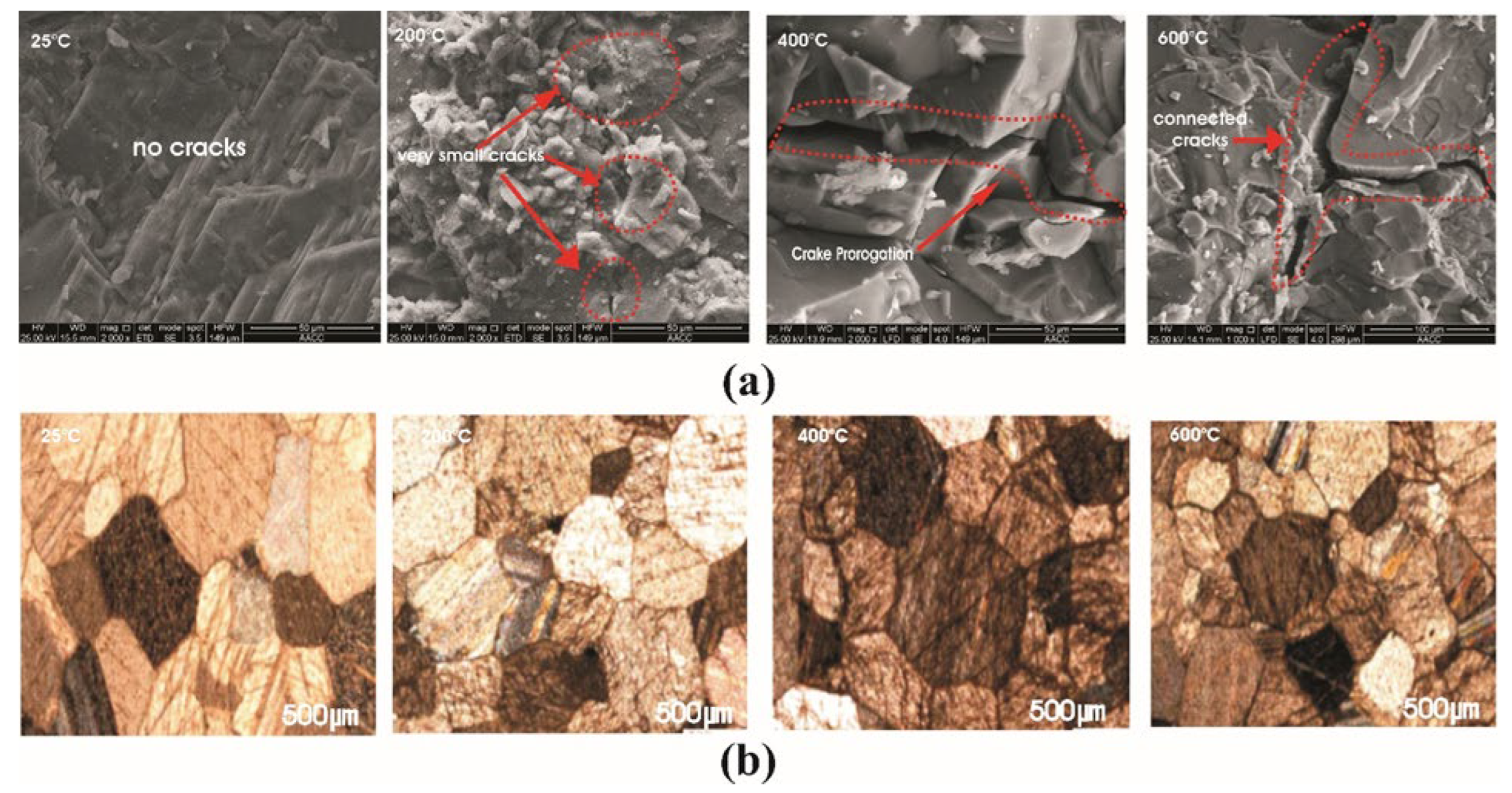
4.2. Micro Crack Analysis

The optical microscopy studies revealed that the grain of the marble is homogeneous. The samples are mainly composed of calcite and show the euhedral shape of crystals with perfect rhombohedral cleavages. Figure 5 depict that the calcite minerals and grain are considerably affected by thermal heat. The crack in the mineral and at the boundary of interlock increase with temperature as shown in Figure 7a, while minerals boundary and their interlock at high resolution were shown in Figure 7b. When temperature increases from 25 °C to 600 °C, more micro-cracks were produced, which also propagated along the existing crack lengths. The samples at room temperature (25 °C), as shown in Figure 7a,b, contains no cracks and the grains are well cemented. While increasing the temperature from room temperature to 200 °C and 400 °C, the separation of some grains, more cracks, and, especially, micro-cracks at grain boundaries were observed in Figure 7a,b. Furthermore, when the temperature was increased to 600 °C, the trans-granular micro-cracks were detected, as shown in Figure 7a,b.

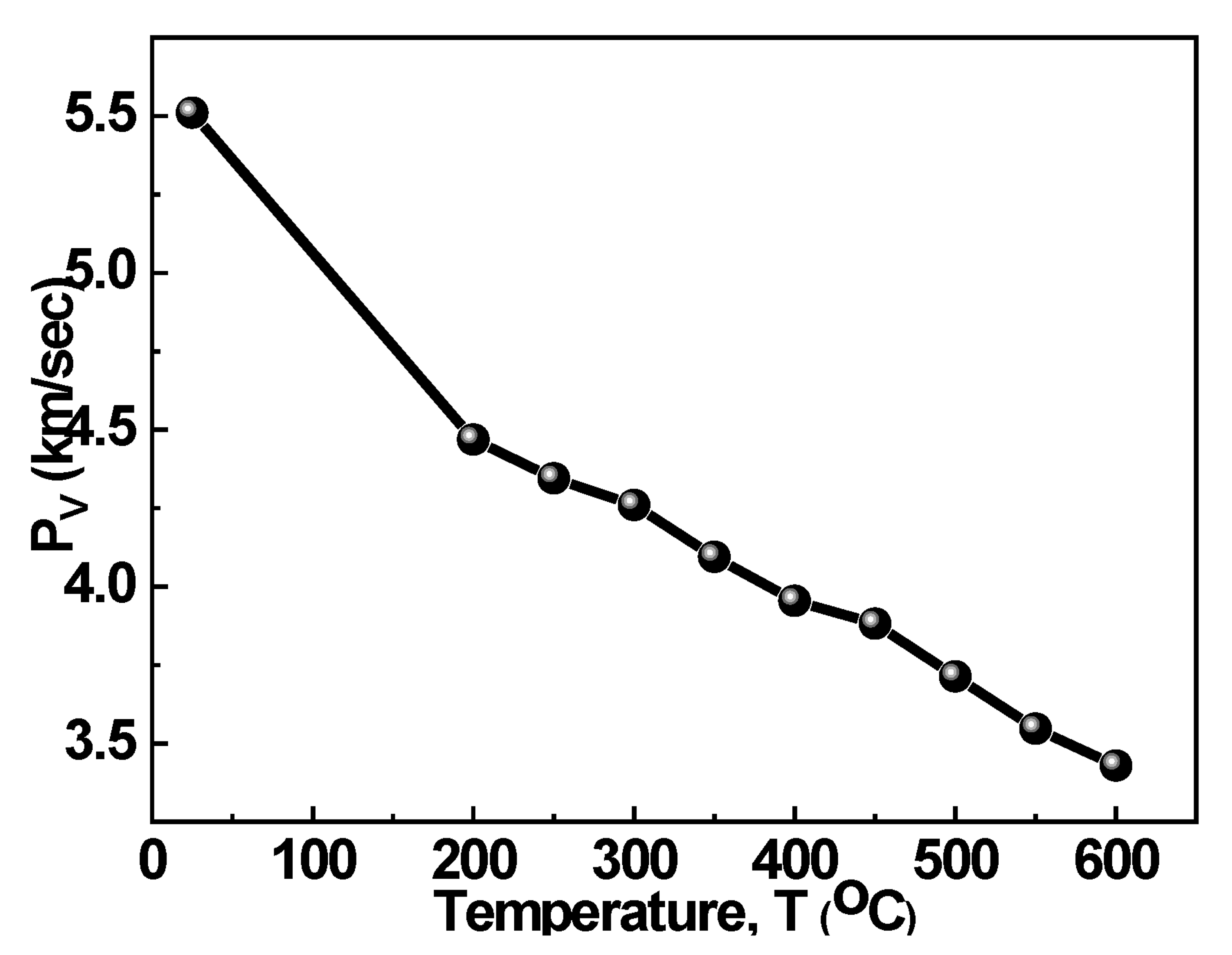
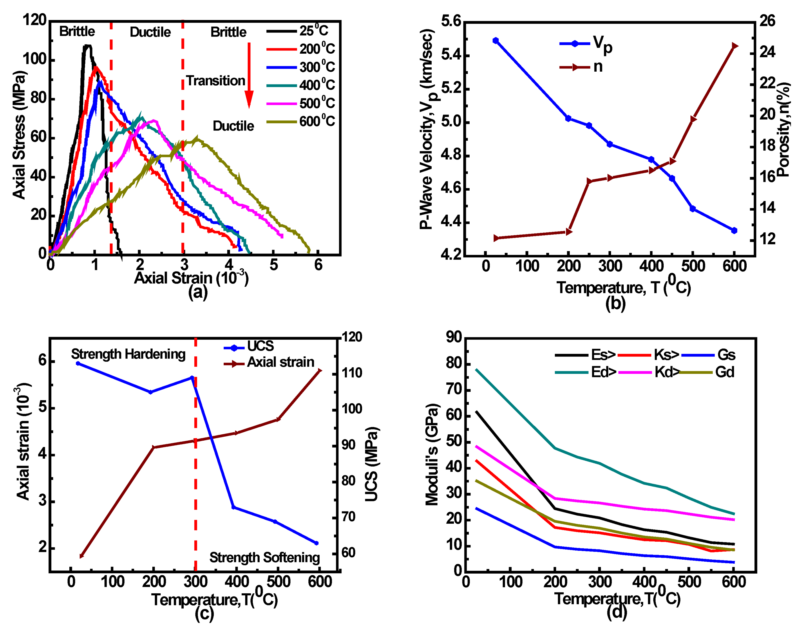
4.3. P-Wave Analysis

The wave velocities traveled differently in the specimens at different temperatures, and this is shown in Figure 6. It can be seen from Figure 8 that the velocity of the wave travel decreases with the temperature increase. This decrease is due to the micro-crack generation, and to the existence of a crack and its extension in length, because wave velocity is sensitive to different mediums. When a crack occurred in rocks, the wave velocity spread slower in air than solid rocks, a pattern which is matched with the experimental results. The trend is presented in Figure 8.

4.4. Effect of Temperature on Stress–Strain Curve

The two parameters of rocks that play a significant role in engineering structure stability are UCS and ES. The temperature effect on the stress–strain behaviors is shown in Figure 9a. A gradual increase in temperature has decreased both the UCS and ES. Figure 9a shows the complete stress–strain curve at different temperatures. The pre-peak stress–strain is significantly influenced by temperature. Temperature variation illustrated a significant influence on stress–strain relations. The initial deformation of the non-linearity pattern increases in the stress–strain curve as the temperature increases. The stress–strain curves shape reveals that, as the temperature increases, the number of micro-cracks is increased and, as a result, the stress decreased. This is in agreement with the changes in material properties from brittle to ductile. The marble rock’s overall ductility increases with the increase in thermal heat, showing a strong agreement with the results of [15].
The marble test results are summarized in Table 3. The result revealed the average UCS, ES, PV, and ρ inverse relation with the increase in temperature, while the strain, as well as η, shows a direct relationship, as indicated in Figure 9b,c. The value of UCS decreased at the temperature range of 25–200 °C, but showed an increase at 200–300 °C, which shows a resemblance to a previous study [70]. On the other hand, at temperatures above 300 °C, the UCS decreased again. The increase in η and decrease in PV are in strong agreement with [71]. Overall, the ES decreased with an increase in temperature, as shown in Figure 9d.

5. Prediction Models of UCS and ES

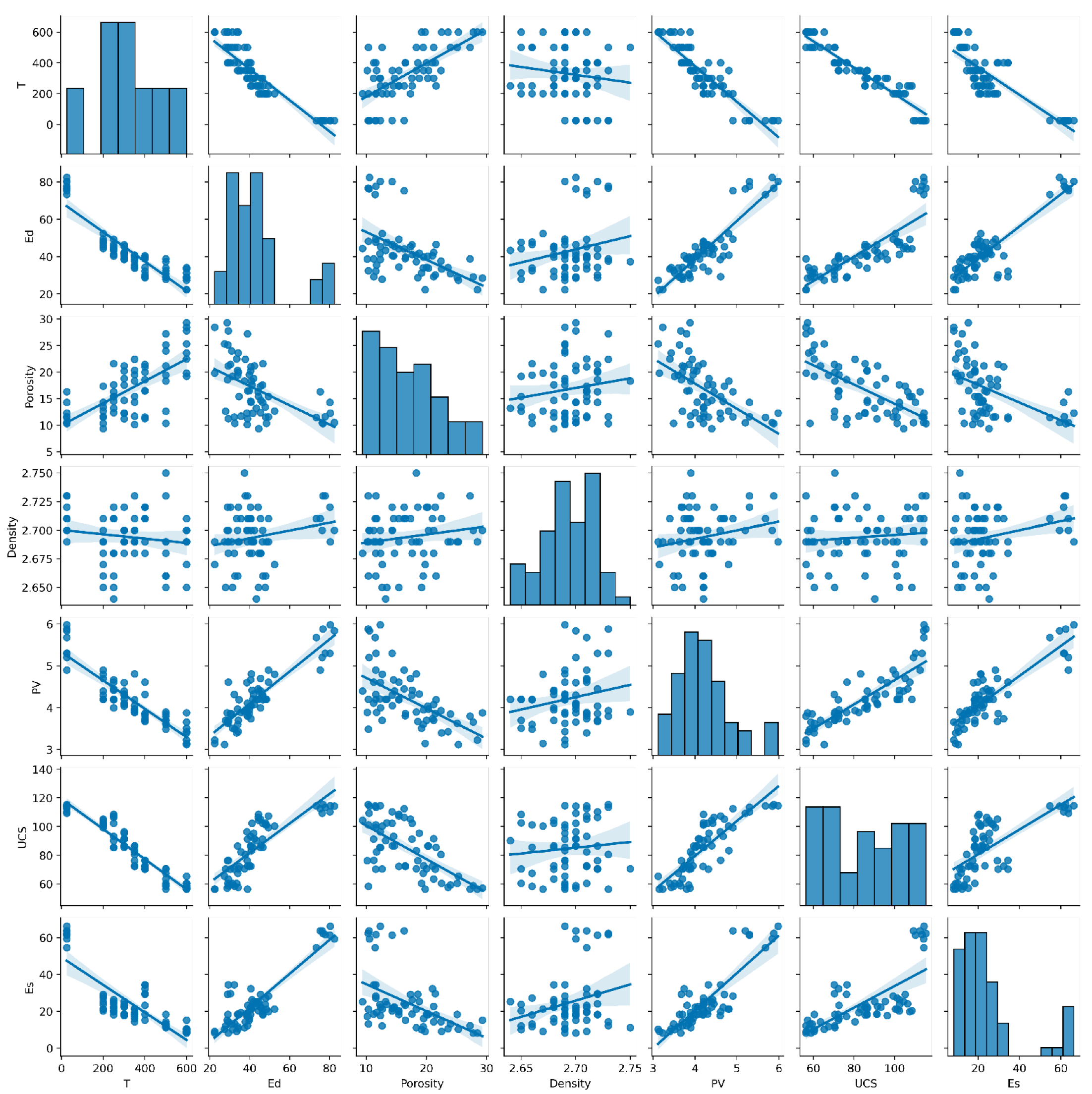
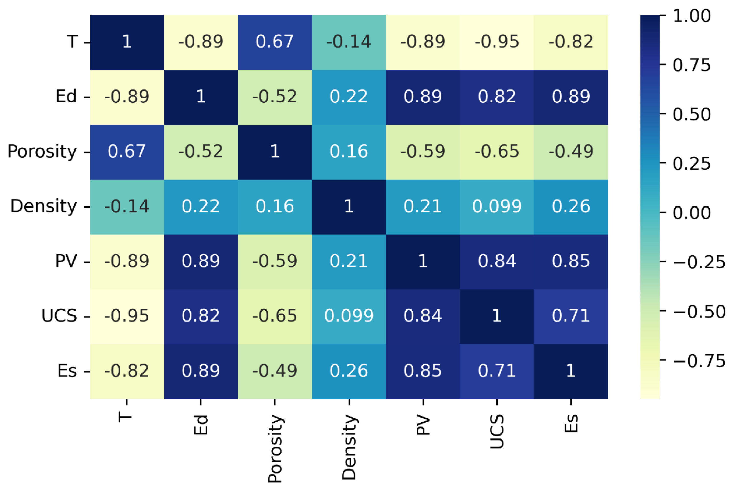
5.1. Preliminary Data Analysis

This study consists of the parameters T, PV, ρ, η, Ed, UCS, and Es for machine learning and a statistical approach. The T, PV, ρ, η, Ed are used as input for the prediction of UCS and Es. The statistical analysis of the inputs and outputs data is described in Table 4.
A correlation matrix is a descriptive statistical tool that informs us about the variance and covariance of regressions that are included in the prediction model. It is often used in conjunction with other statistical matrices. Correlation, on the other hand, describes the regression variations with each other in predictive analysis. In general, the correlation matrix explains the variation of each variable. This can be shown in Figure 10 and Figure 11 with correlation and pairwise correlation, respectively. This revealed that the inputs variables have negative relationship, positive relationship, and no relationship with outputs and each other. For example, temperature and density have a negative relationship, but this relationship is weak, PV have a positive correlation, while other inputs and output have a negative correlation. Figure 10 and Figure 11 enable a researcher to easily understand the effect of inputs on output results of the predicted model. The greater the negative or positive relationship, the greater will be the importance in model efficiency.

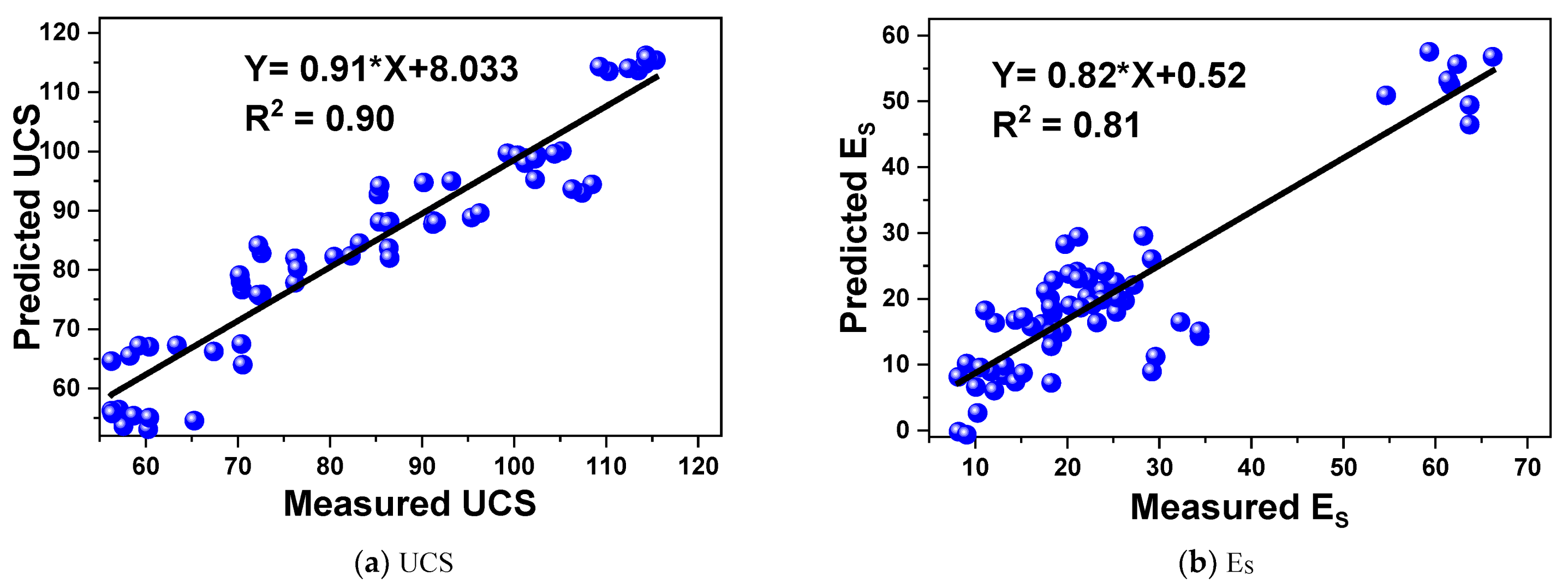
5.2. MLR Prediction Models

Two different multilinear regression equations were developed for the prediction of UCS and Es, respectively. These can be mathematically expressed using Equations (5) and (6), as follows:
U C S = 186.017 0.116 T 0.232 E d + 0.078 η 24.41 ρ + 2.694 P v
E s = 164.9 + 0.003 T + 0.657 E d 0.098 η + 49.318 ρ + 6.890 P v
where UCS is uniaxial compressive strength (Mpa) and Es is the static Young’s modulus (GPa), T is temperature (°C), Ed is the dynamic Young’s modulus (GPa), η is porosity (%), ρ is density (gr/cm3), and PV is P-wave velocity (km/s).
The fundamental descriptive statistic of the original data is shown in Table 3 and Table 4.

Importance of Variable in MLR Models

The MLR model for the UCS has a high coefficient of determination (R2) between the actual and predicted UCS (R2 = 0.90), as shown in Figure 12a. In the UCS model, out of five independent variables, two variables are highly correlated with UCS, namely T and PV, and give a significant value less than (p = 0.05), while the other three parameters, namely ρ, η, and Ed, have less significance because of their P-value is greater than 0.05. The ES model gives an effective coefficient of determination (R2 = 0.817), as shown in Figure 12b. In this model, out of five parameters, the two parameters which are highly correlated with ES are PV with a significance value (p = 0.042), and T, with significance value (p = 0.036), while Ed is worthless. The other two variables, porosity and density, have a significance level more than 0.05, namely η (0.693) and ρ (0.238). These models revealed that the PV and T have a dominant effect on both models of UCS and ES, while the other three parameters have shown no obvious significance in both models.

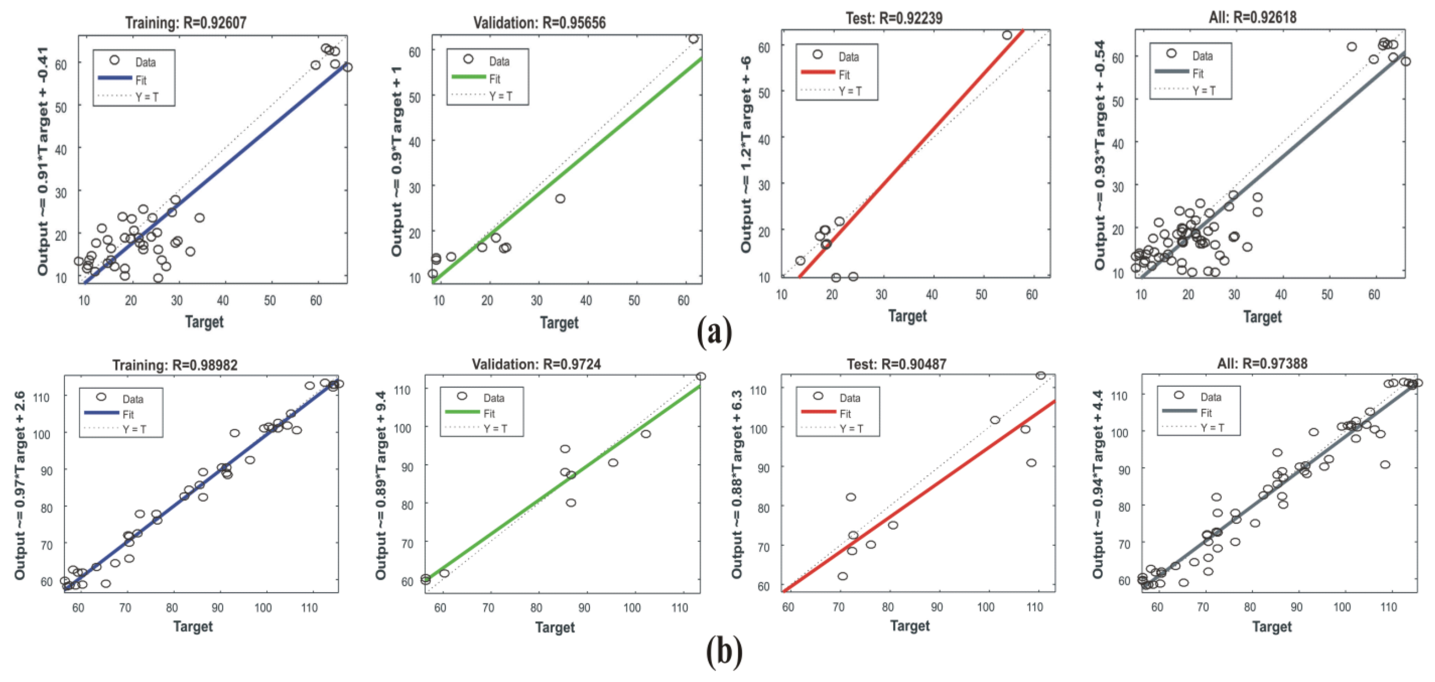
5.3. Network Phases and Regression Model

Each phase of the ANN, i.e., training, validation, testing, and the regression values are shown in Figure 13a,b for the UCS and ES models. The good regression is achieved in training and validation, and testing values between the predicted and measured values of UCS as shown in Figure 13b. In the case of ES, the regression values of the predicted and measured show high validation regression values, as presented in Figure 13a. The plot draws from the ANN model are shown in Figure 14a,b. A good R2 value (0.95) between the predicted and measured UCS is found as shown in Figure 14a. Figure 14b shows a relatively lesser coefficient of determination value (0.85) between predicted ES and measured ES, as compared to predicted and measured UCS.

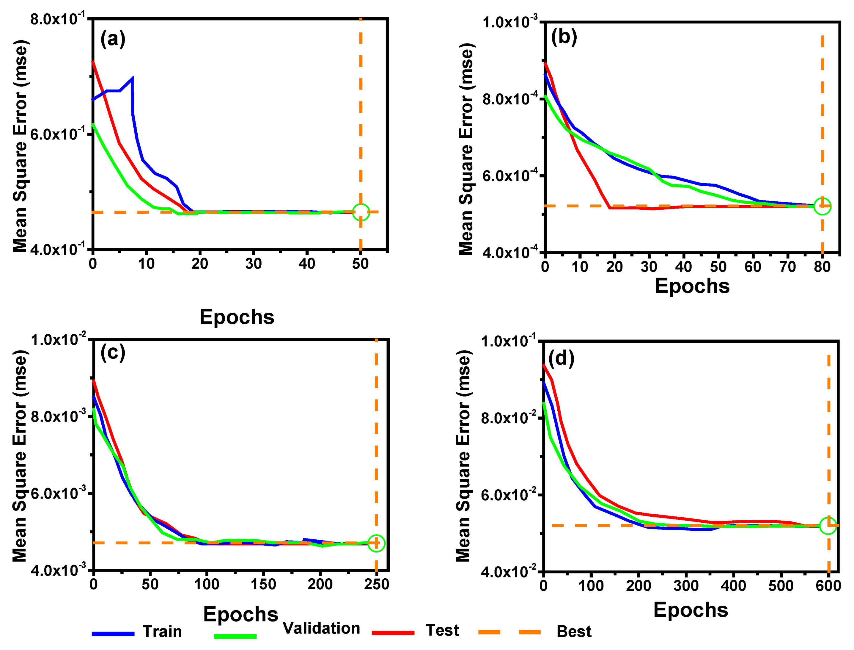
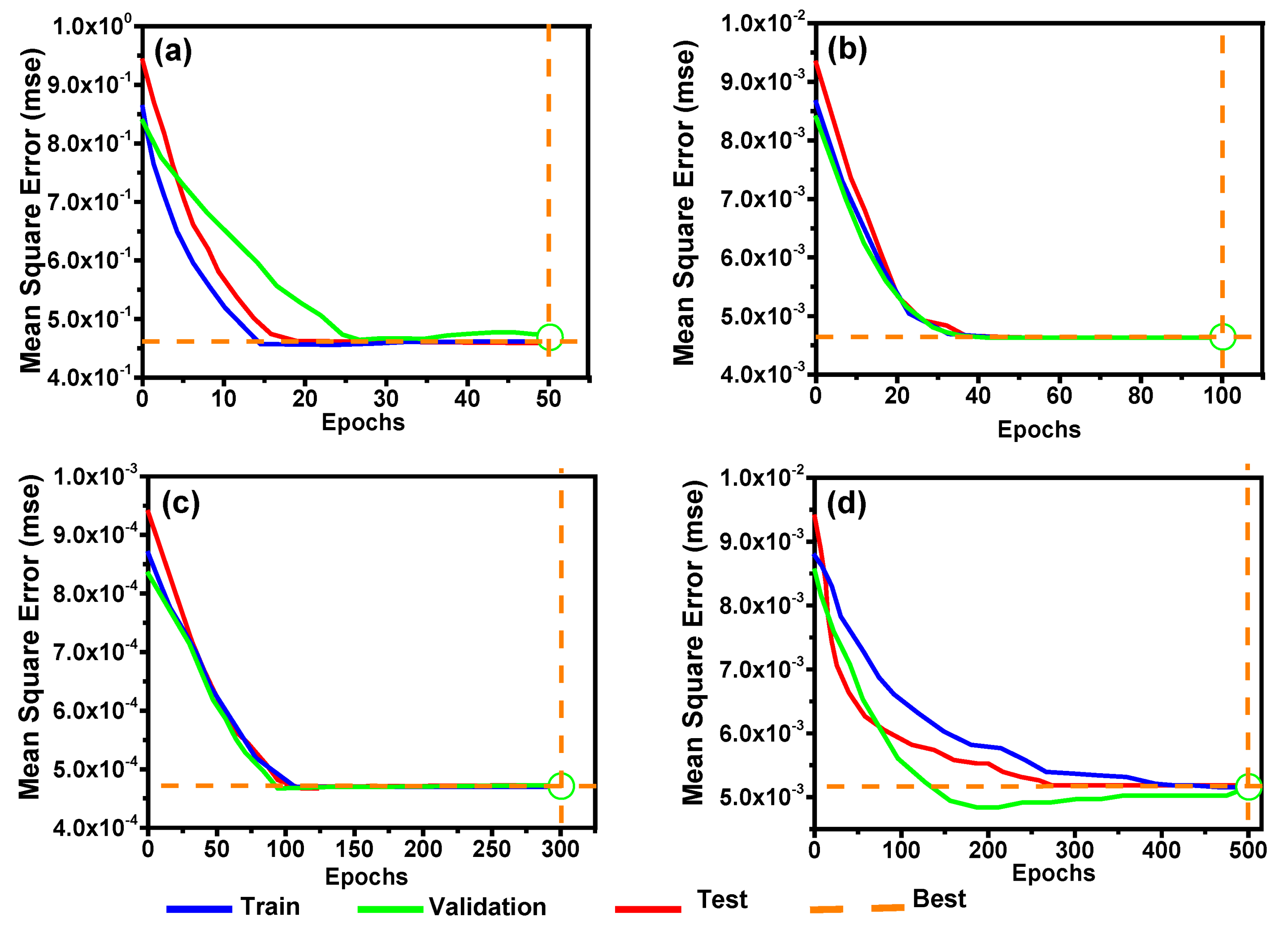
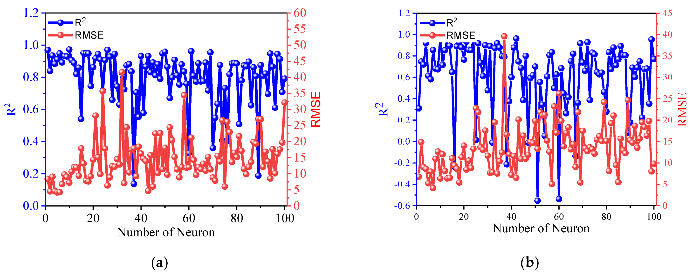
5.3.1. Network Performance and Accuracy

The network performance and accuracy are evaluated by means of MSE (mean squared error) value. The MSE value decreases as the number iteration increased by increasing the neuron number of the hidden layer. For each model of UCS and ES, the MSE is evaluated separately. The optimum regression model is achieved through a lesser MSE value at 250 and 300 epochs for UCS and ES, respectively, as shown in Figure 15 and Figure 16. This also revealed the number of iteration and number of neuron play key role in the accuracy achievement of the model. that The neuron convergence analysis shows that the optimum regression and least MSE for UCS and ES are obtained on 5 and 7 neurons, respectively, as shown in Figure 17.

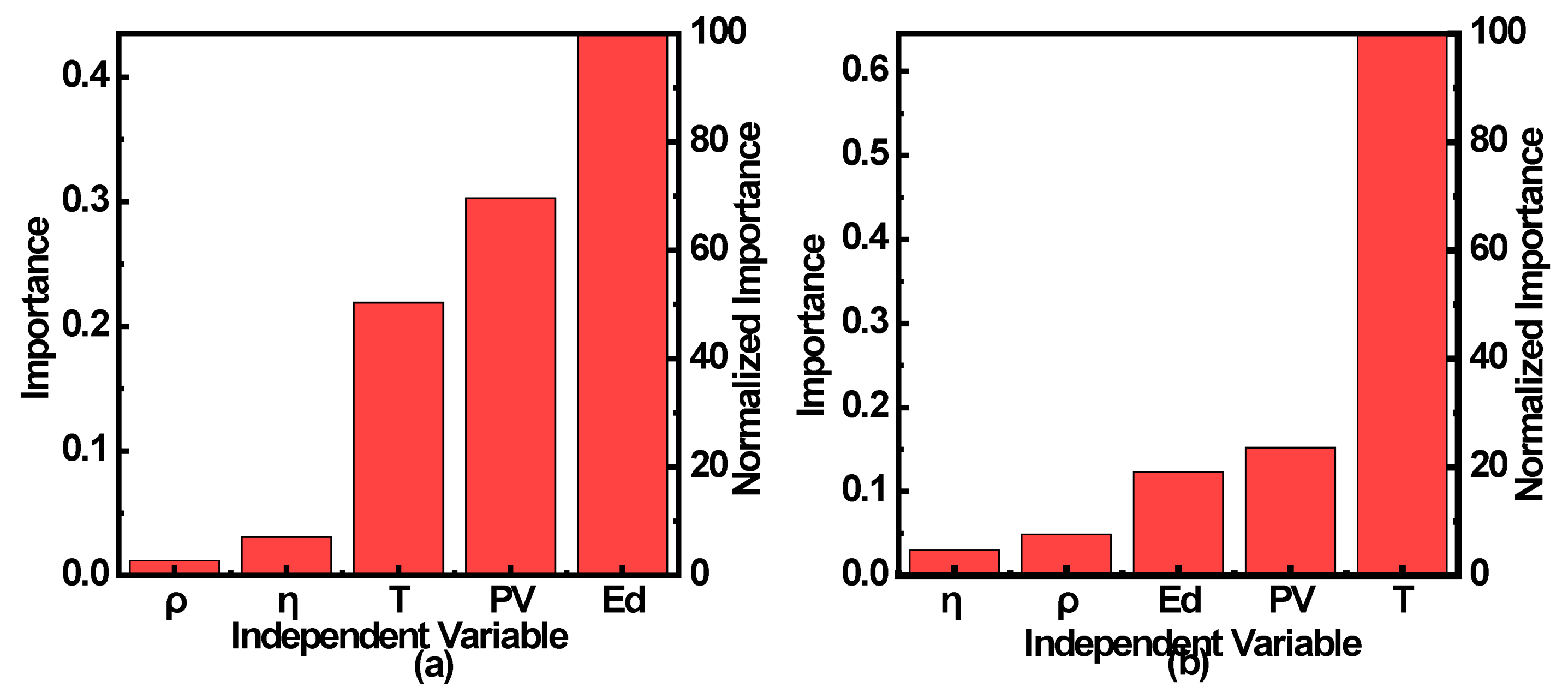
5.3.2. Importance of Variable in ANN Models
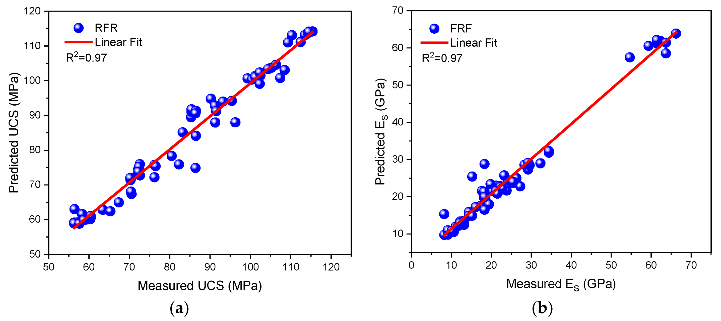
The importance of the ANN independent variable for UCS and ES is shown in Figure 18a,b. In Figure 18a, it seems that the Ed, PV, and T show a strong relation with ES, while ρ and η show a weak relation to ES. The independent variable, such as T, PV, and Ed, have a strong relation with UCS, the most important of which is temperature, as shown in Figure 18b. Moreover, ρ and η have a very low relation to UCS.

5.4. Random Forest

The Scikit-Learn package in Python was used to construct the random forest regression (RFR) and k-nearest neighbor’s regression (KNN) models. It is a Python package that contains several different machine learning algorithms that are easily accessible for use in various applications. At the beginning of this research project, the data were normalized in order to adapt the values that were measured on various scales to a standard scale. After this, the models were trained on 70% of the data, and the remaining 30% of the data was split into two equal portions, namely the testing set (15%) and the validation set (15%). The hyperparameters were fine-tuned with the help of the testing set. In the RFR model, the hyperparameters, referred to as “n_estimators” and “max_depth”, were subjected to a range of different values. Before calculating the maximum averages of predictions, the number of estimators refers to the number of decision trees that were constructed by the random forest regression model. The model becomes more computationally costly as the number of trees increases, but it also provides improved performance. The depth of each decision tree that makes up a random forest is represented by the maximum depth hyperparameters. The model is overfitted, since it was given a value for the maximum depth hyperparameter that was very high. The optimum value of n_estimators, max_depth, and random_state is described in Table 5. Furthermore, the predicted value at this optimum parameter’s value has a high correlation coefficient (R2 = 0.97) for USC and ES, as shown in Figure 19.

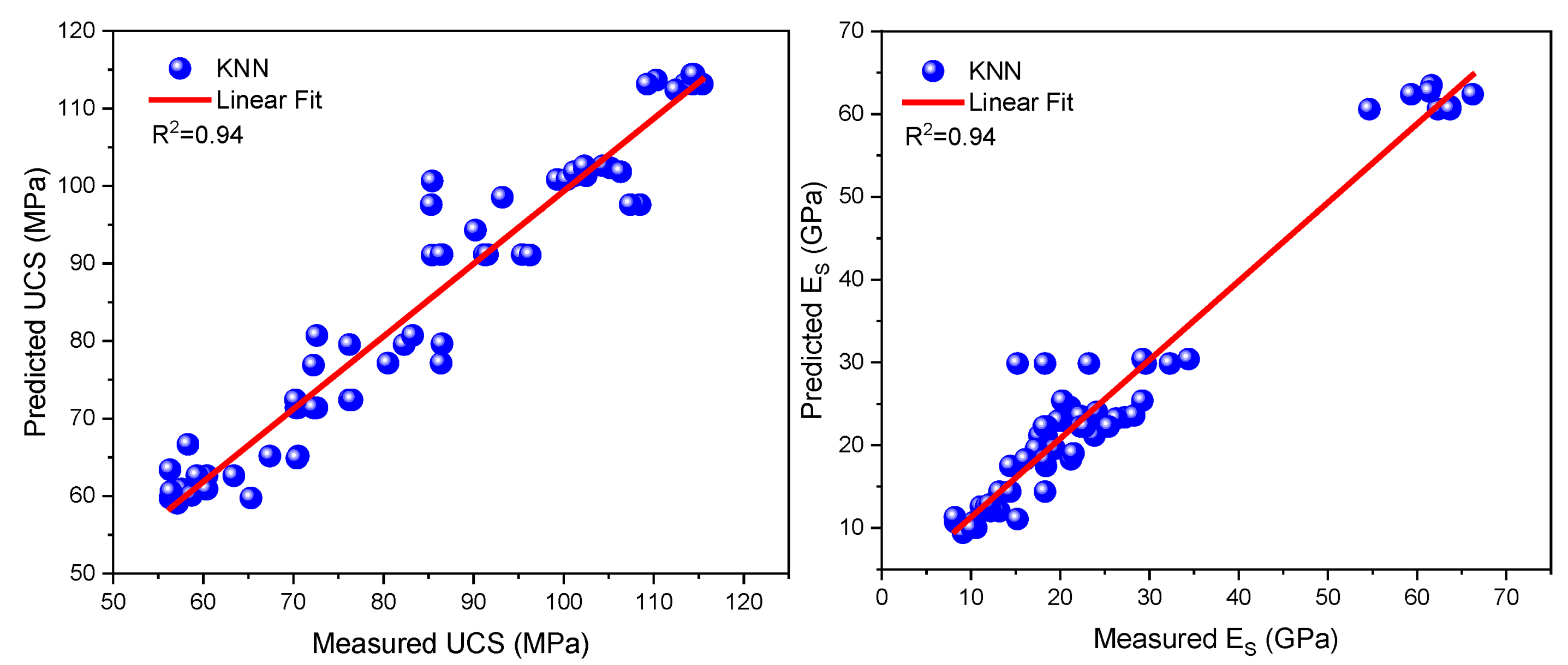
5.5. k-Nearest Neighbor

In the KNN model, the number of neighbors, denoted by the variable “n_neighbors,” was subject to change. When making a forecast, the number of neighbors that should be included in the averaging process is specified by a hyperparameter referred to as the “number of neighbors.” When the value of the n_neighbors hyperparameter is increased to a large number, the method becomes more accurate but also more computationally intensive. The grid search approach was used in order to arrive at the ideal values for the hyperparameters. The grid search approach determines the optimal combination by testing a broad variety of possible values for each hyperparameter that is being changed and then selecting one of those values. However, when working with huge datasets, it is computationally costly to pick the optimal combination of hyperparameters by selecting a broad range for each hyperparameter. This is done in order to maximize the accuracy of the results. In order to determine a workable range for each hyperparameter, the value was played about with on a number of different levels while the other hyperparameters remained the same. The range of values within which the “number of estimators” and “max depth” hyperparameters have an effect on the RFR model’s performance. Table 6 has a description of the ideal combination of n neighbors and metric values. In addition, the projected value at this optimal value for the parameters has a good correlation coefficient (R2 = 0.94), as can be shown in Figure 20. This is the case for both USC and ES.

6. A Comparative Evaluation of Statistics and Intelligent Techniques

The comparison of correlation efficiencies of various developed models was used in this study to improve the performance of predicted models. Through this comparison, the subsequent performance indices, such as R2, MAPE, RMSE, and VAF, were evaluated. An excellent model can be represented by performance indices as, R2 = 1, MAPE = RMSE = 0, and VAF = 100%. The performance indices were calculated using Equations (7)–(10), as follows:
R 2 = i = 1 n ( y i ) 2 i = 1 n ( y i k i ) 2 i = 1 n ( y i ) 2
MAPE = 1 2 i = 1 n y i k i y i × 100
RMSE = i = 1 n ( y i k i ) n
VAF = 1 var ( y k ) var ( y )   x   100
where, y is the actual value, and k′ is the predicted value.
Table 7 describe the performance indices of all models. This shows that the MLR gives a lower coefficient of determination for both predicted parameters, while RFR gives a high coefficient of determination for UCS and ES. On the basis of this performance indices, the RFR performed well.

7. Discussion

(1) Predictive models were developed for UCS and ES based on statistical (MLR) and intelligent models (ANNs, RFR, and KNN). The accuracy and performance of models are satisfactory on the basis of MSE, MAPE, VAF, and R2. The MSE, MAPE, VAF of the MLR is greater than that of the intelligent models. The intelligent models have shown a better prediction performance than the statistical model due to its MSE, MAPE, VAF values and high R2 value. The MSE, MAPE, VAF, R2 values of the MLR are fixed, while the MSE, MAPE, VAF and R2 of the intelligent model are varied. It depends on the neuron optimization in the hidden layer for ANN and the hyperparameters. The MSE, MAPE, and VAF of a prediction model can improve through trial and error methods using an intelligent model. The intelligent model’s optimization needs an expert person who can know the tuning the of hyperparameters number, and how to fine-tune hyperparameters to obtain more reliable results.
(2) The intelligent models with high correlation for UCS and ES respectively are better, as shown in Figure 14a,b, Figure 19a,b, and Figure 20a,b, than MLR. In this research work, ANN gives 5% for UCS and 4% for ES, RFR give 7% for UCS and 16% for ES, and gives 4% for UCS and 13% for ES, meaning that the intelligent model is more accurate than the MLR. Furthermore, RFR give 7% for UCS and 16% for ES, which is more accurate than the statistical model and has 4-5% high accuracy than ANN and KNN. The models are based on limited data and only valid to a specific area. The models can extend to a generalized form in the future to take a large amount of data on different rocks. Temperature and P-wave velocity are strongly correlated in both models. The three other input parameters play a worthless role in the equation. This work result is strongly supported by existing research [35]. It suggested PV, ρ, and η as input variables and, after prediction, revealed that only P-wave velocity has a strong correlation, and the other input variables have a worthless contribution. This study is based on thermal effect; therefore, the temperature is considered as an input parameter that has a strong influence on the mechanical and physical properties of rock. Furthermore, in these modes, the temperature and P-wave velocity both have a strong correlation with output, and the other three independent parameters are meaningless in the model. The performance of this model is better than in the model developed by Torabi-Kaveh, Naseri, Saneie, and Sarshari [26].
(3) After a comparative analysis of results obtained from MLR and the intelligent model, it is concluded that the intelligent model gives effective results as compared to MLR in predicting UCS and ES. The variable performance in both MLR and the intelligent model shows that the T and PV played an active role in the prediction models, while the ρ, η, and Ed have a less active predictive role.
(4) An important factor in marble’s anisotropic behaviour is its temperature state, which may directly influence the material’s characteristics and cause the cohesiveness along the grain boundary to weaken [15]. Although anisotropy has a significant impact on the physico-mechanical behaviour of intact and discontinuous geomaterials, it is often neglected in day-to-day geoengineering practice. This is despite the fact that it is an essential property. The presumption that anisotropic rocks have isotropic properties can primarily be explained by the following factors: (i) the complicated structure of anisotropic elasticity theory; (ii) the increased number of moduli required to describe the deformational behaviour of anisotropic materials; (iii) the significant challenges associated with the reliable sampling and testing of anisotropic geomaterials; (iv) the inherent difficulties of back analysis methodologies related to anisotropic rock. There are extremely few examples of completely isotropic rocks and soils in the natural world. Numerous rock properties, such as thermal conductivity, coefficient of thermal expansion, and other physical (electrical, magnetic, etc.) characteristics, as well as the deformational and strength characteristics of soils and rocks, may be directionally reliant on antecedent endogenetic (primary) or exogenetic (secondary) causes that occur at micro-, meso-, and macroscales. This may be the case for many rock properties, including thermal conductivity, coefficient of thermal expansion, and other physical properties (electrical, magnetic, etc). The former refers to the processes of sedimentation, compaction, and lithification that are responsible for the formation of sedimentary rock formations (such as limestones, sandstones, and other similar rocks), whereas the latter refers to environmental factors, such as pressure, temperature, chemical solutions, and other similar elements that are also responsible for the transformation of various rock types (i.e., diagenesis, metamorphosis, weathering, etc.). Crystallographic preferred orientations (textures) of the rock components, grain shape fabric, and microcrack fabric are principally responsible for influencing the anisotropic physical features of intact rocks at the microscopic and mesoscopic scales, respectively. At the macroscopic level, the anisotropic character of discontinuous rocks is reflected in the foliation, cleavage, and fractures that make up these rocks [71]. The influence of anisotropic characteristics will be taken into consideration in the prediction model that uses computer tomography in the near future.

8. Conclusions

The following conclusions are drawn from the research:
  • The physical and mechanical properties are greatly affected by the increase in temperature from 200–600 °C due to the generation and propagation of micro-cracks. The porosity is increased, while PV is decreased with the increase in temperature. The strength properties i.e., UCS and ES, of rock also decrease with the increasing temperature;
  • The behavior of the stress–strain curve is changed from brittle to ductile when the temperature is increased;
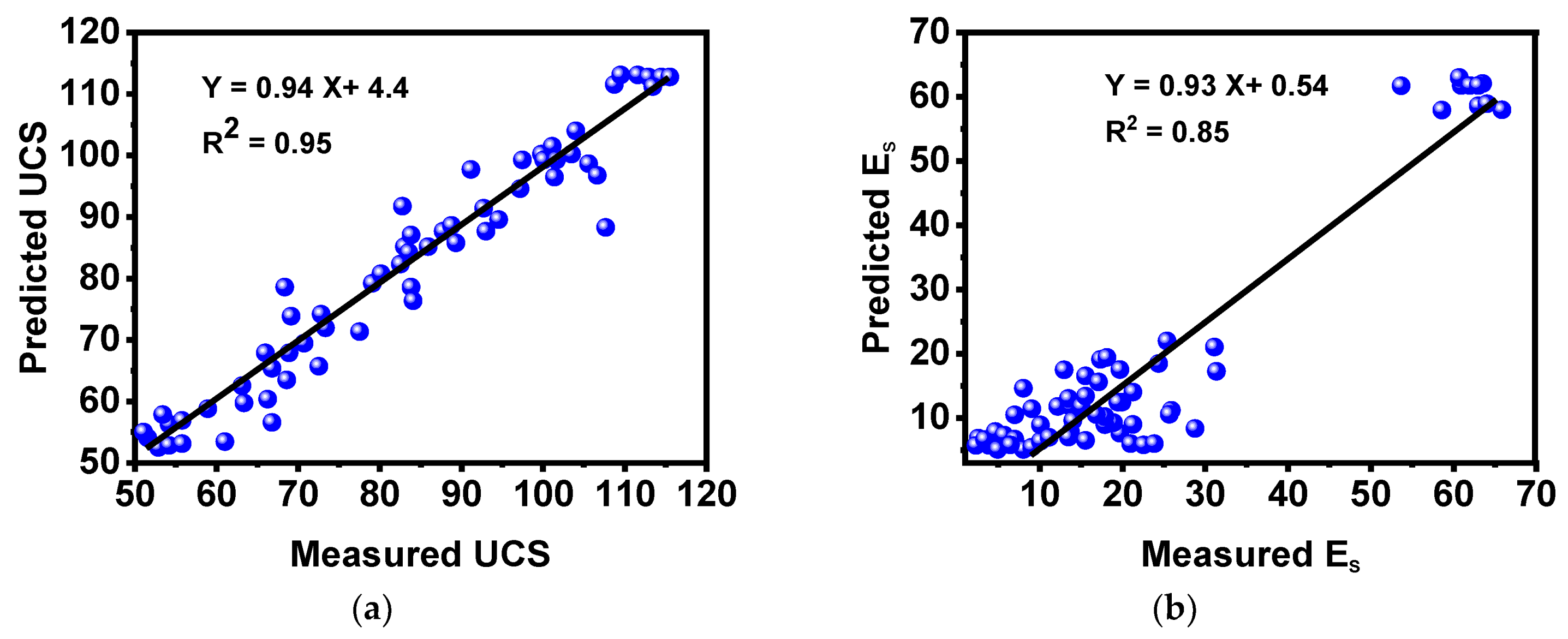
  • The MLR predictive models for UCS and ES give a performance coefficient of 0.90% and 0.81%, respectively. The intelligent models i.e., ANN, RFR, and KNN for UCS and ES give a performance coefficient, revealing that the model for UCS is (5–7%) and ES is (4–16%) better than the statistical model (MRL models).
  • The model’s important feature revealed that the temperature and PV have a significant role in prediction models;
  • Based on comparative analysis of MLR, ANN, RFR, and KNN, it has been proposed that RFR model is suitable for use in the prediction of UCS and ES under thermal treatment.

Author Contributions

N.M.K. and S.H. contributed to the research, designed experiments and wrote the paper. Q.Y. and M.Z.E. conceived this research and were responsible for the research. H.R. supervised this study. M.H.B.M.H. and K.C. contributed in the original as well as in the revised version of the manuscript. H.R., S.K., K.S.S. and B.U. reviewed and revised the paper. All authors have read and agreed to the published version of the manuscript.

Funding

This research received no external funding.

Informed Consent Statement

Not applicable.

Data Availability Statement

All the data and models employed and/or generated during the study appear in the submitted article.

Conflicts of Interest

The authors declare no conflict of interest.

References

  1. Qin, Y.; Tian, H.; Xu, N.-X.; Chen, Y. Physical and mechanical properties of granite after high-temperature treatment. Rock Mech. Rock Eng. 2020, 53, 305–322. [Google Scholar] [CrossRef]
  2. Vagnon, F.; Colombero, C.; Colombo, F.; Comina, C.; Ferrero, A.M.; Mandrone, G.; Vinciguerra, S.C. Effects of thermal treatment on physical and mechanical properties of Valdieri Marble-NW Italy. Int. J. Rock Mech. Min. Sci. 2019, 116, 75–86. [Google Scholar] [CrossRef]
  3. Gautam, P.; Verma, A.; Jha, M.; Sharma, P.; Singh, T.N. Effect of high temperature on physical and mechanical properties of Jalore granite. J. Appl. Geophys. 2018, 159, 460–474. [Google Scholar] [CrossRef]
  4. Lin, K.; Huang, W.; Finkelman, R.B.; Chen, J.; Yi, S.; Cui, X.; Wang, Y.J. Distribution, modes of occurrence, and main factors influencing lead enrichment in Chinese coals. Int. J. Coal Sci. Technol. 2020, 7, 1–18. [Google Scholar] [CrossRef] [Green Version]
  5. Liu, S.; Tan, F.; Huo, T.; Tang, S.; Zhao, W.; Chao, H.J. Origin of the hydrate bound gases in the Juhugeng Sag, Muli Basin, Tibetan Plateau. Int. J. Coal Sci. Technol. 2020, 7, 43–57. [Google Scholar] [CrossRef] [Green Version]
  6. Chen, L.; Mao, X.; Wu, P. Effect of High Temperature and Inclination Angle on Mechanical Properties and Fracture Behavior of Granite at Low Strain Rate. Sustainability 2020, 12, 1255. [Google Scholar] [CrossRef] [Green Version]
  7. Zhang, W.; Wang, T.; Zhang, D.; Tang, J.; Xu, P.; Duan, X. A Comprehensive Set of Cooling Measures for the Overall Control and Reduction of High Temperature-Induced Thermal Damage in Oversize Deep Mines: A Case Study. Sustainability 2020, 12, 2489. [Google Scholar] [CrossRef] [Green Version]
  8. Gomah, M.E.; Li, G.; Sun, C.; Xu, J.; Yang, S.; Li, J. On the Physical and Mechanical Responses of Egyptian Granodiorite after High-Temperature Treatments. Sustainability 2022, 14, 4632. [Google Scholar] [CrossRef]
  9. Meng, Q.-B.; Wang, C.-K.; Liu, J.-F.; Zhang, M.-W.; Lu, M.-M.; Wu, Y. Physical and micro-structural characteristics of limestone after high temperature exposure. Bull. Eng. Geol. Environ. 2020, 79, 1259–1274. [Google Scholar] [CrossRef]
  10. Lian, X.; Hu, H.; Li, T.; Hu, D. Main geological and mining factors affecting ground cracks induced by underground coal mining in Shanxi Province, China. Int. J. Coal Sci. Technol. 2020, 7, 362–370. [Google Scholar] [CrossRef] [Green Version]
  11. Zuo, J.; Wang, J.; Jiang, Y. Macro/meso failure behavior of surrounding rock in deep roadway and its control technology. Int. J. Coal Sci. Technol. 2019, 6, 301–319. [Google Scholar] [CrossRef] [Green Version]
  12. Barla, G. Comprehensive study including testing, monitoring and thermo-hydro modelling for design and implementation of a geothermal system in Torino (Italy). Geomech. Geophys. Geo-Energy Geo-Resour. 2017, 3, 175–188. [Google Scholar] [CrossRef]
  13. Breede, K.; Dzebisashvili, K.; Liu, X.; Falcone, G. A systematic review of enhanced (or engineered) geothermal systems: Past, present and future. Geotherm. Energy 2013, 1, 4. [Google Scholar] [CrossRef] [Green Version]
  14. Homand-Etienne, F.; Houpert, R. Thermally induced microcracking in granites: Characterization and analysis. Int. J. Rock Mech. Min. Sci. Geomech. Abstr. 1989, 26, 125–134. [Google Scholar] [CrossRef]
  15. Peng, J.; Rong, G.; Cai, M.; Yao, M.-D.; Zhou, C.-B. Physical and mechanical behaviors of a thermal-damaged coarse marble under uniaxial compression. Eng. Geol. 2016, 200, 88–93. [Google Scholar] [CrossRef]
  16. Ferreira, A.P.G.; Farage, M.C.; Barbosa, F.S.; Noumowé, A.; Renault, N. Thermo-hydric analysis of concrete–rock bilayers under fire conditions. Eng. Struct. 2014, 59, 765–775. [Google Scholar] [CrossRef]
  17. Tang, Z.C.; Sun, M.; Peng, J. Influence of high temperature duration on physical, thermal and mechanical properties of a fine-grained marble. Appl. Therm. Eng. 2019, 156, 34–50. [Google Scholar] [CrossRef]
  18. Jansen, D.P.; Carlson, S.R.; Young, R.P.; Hutchins, D.A. Ultrasonic imaging and acoustic emission monitoring of thermally induced microcracks in Lac du Bonnet granite. J. Geophys. Res. Solid Earth 1993, 98, 22231–22243. [Google Scholar] [CrossRef]
  19. Dwivedi, R.D.; Goel, R.K.; Prasad, V.V.R.; Sinha, A. Thermo-mechanical properties of Indian and other granites. Int. J. Rock Mech. Min. Sci. 2008, 45, 303–315. [Google Scholar] [CrossRef]
  20. Zhao, Y.; Wan, Z.; Feng, Z.; Yang, D.; Zhang, Y.; Qu, F. Triaxial compression system for rock testing under high temperature and high pressure. Int. J. Rock Mech. Min. Sci. 2012, 52, 132–138. [Google Scholar] [CrossRef]
  21. Wong, T.-F. Effects of temperature and pressure on failure and post-failure behavior of Westerly granite. Mech. Mater. 1982, 1, 3–17. [Google Scholar] [CrossRef]
  22. Chaki, S.; Takarli, M.; Agbodjan, W.P. Influence of thermal damage on physical properties of a granite rock: Porosity, permeability and ultrasonic wave evolutions. Constr. Build. Mater. 2008, 22, 1456–1461. [Google Scholar] [CrossRef]
  23. Lion, M.; Skoczylas, F.; Ledésert, B. Effects of heating on the hydraulic and poroelastic properties of bourgogne limestone. Int. J. Rock Mech. Min. Sci. 2005, 42, 508–520. [Google Scholar] [CrossRef]
  24. Malaga-Starzec, K.; Åkesson, U.; Lindqvist, J.E.; Schouenborg, B. Microscopic and macroscopic characterization of the porosity of marble as a function of temperature and impregnation. Constr. Build. Mater. 2006, 20, 939–947. [Google Scholar] [CrossRef]
  25. Chen, Y.-L.; Ni, J.; Shao, W.; Azzam, R. Experimental study on the influence of temperature on the mechanical properties of granite under uni-axial compression and fatigue loading. Int. J. Rock Mech. Min. Sci. 2012, 56, 62–66. [Google Scholar] [CrossRef]
  26. Torabi-Kaveh, M.; Naseri, F.; Saneie, S.; Sarshari, B. Application of artificial neural networks and multivariate statistics to predict UCS and E using physical properties of Asmari limestones. Arab. J. Geosci. 2015, 8, 2889–2897. [Google Scholar] [CrossRef]
  27. Heidari, M.; Khanlari, G.; Momeni, A. Prediction of Elastic Modulus of Intact Rocks Using Artificial Neural Networks and non-Linear Regression Methods. Aust. J. Basic Appl. Sci. 2010, 4, 5869–5879. [Google Scholar]
  28. Abdi, Y.; Garavand, A.T.; Sahamieh, R.Z. Prediction of strength parameters of sedimentary rocks using artificial neural networks and regression analysis. Arab. J. Geosci. 2018, 11, 587. [Google Scholar] [CrossRef]
  29. Tariq, Z.; Elkatatny, S.; Mahmoud, M.; Ali, A.Z.; Abdulraheem, A. A new approach to predict failure parameters of carbonate rocks using artificial intelligence tools. In Proceedings of the SPE Kingdom of Saudi Arabia Annual Technical Symposium and Exhibition, Dammam, Saudi Arabia, 24–27 April 2017. [Google Scholar]
  30. Manouchehrian, A.; Sharifzadeh, M.; Moghadam, R. Application of artificial neural networks and multivariate statistics to estimate UCS using textural characteristics. Int. J. Min. Sci. Technol. 2012, 22, 229–236. [Google Scholar] [CrossRef]
  31. Dehghan, S.; Sattari, G.; Chehreh Chelgani, S.; Aliabadi, M.A. Prediction of uniaxial compressive strength and modulus of elasticity for Travertine samples using regression and artificial neural networks. Min. Sci. Technol. 2010, 20, 41–46. [Google Scholar] [CrossRef]
  32. Zhang, J.; Ma, G.; Huang, Y.; Aslani, F.; Nener, B.J. Modelling uniaxial compressive strength of lightweight self-compacting concrete using random forest regression. Constr. Build. Mater. 2019, 210, 713–719. [Google Scholar] [CrossRef]
  33. Matin, S.; Farahzadi, L.; Makaremi, S.; Chelgani, S.C.; Sattari, G. Variable selection and prediction of uniaxial compressive strength and modulus of elasticity by random forest. Appl. Soft Comput. 2018, 70, 980–987. [Google Scholar] [CrossRef]
  34. Suthar, M. Applying several machine learning approaches for prediction of unconfined compressive strength of stabilized pond ashes. Neural Comput. Appl. 2020, 32, 9019–9028. [Google Scholar] [CrossRef]
  35. Wang, M.; Wan, W.; Zhao, Y. Prediction of the uniaxial compressive strength of rocks from simple index tests using a random forest predictive model. Comptes Rendus Mec. 2020, 348, 3–32. [Google Scholar] [CrossRef]
  36. Ren, Q.; Wang, G.; Li, M.; Han, S. Prediction of rock compressive strength using machine learning algorithms based on spectrum analysis of geological hammer. Geotech. Geol. Eng. 2019, 37, 475–489. [Google Scholar] [CrossRef]
  37. Ghasemi, E.; Kalhori, H.; Bagherpour, R.; Yagiz, S. Model tree approach for predicting uniaxial compressive strength and Young’s modulus of carbonate rocks. Bull. Eng. Geol. Environ. 2018, 77, 331–343. [Google Scholar] [CrossRef]
  38. Saedi, B.; Mohammadi, S.D.; Shahbazi, H. Prediction of uniaxial compressive strength and elastic modulus of migmatites using various modeling techniques. Arab. J. Geosci. 2018, 11, 574. [Google Scholar] [CrossRef]
  39. Shahani, N.M.; Zheng, X.; Liu, C.; Hassan, F.U.; Li, P. Developing an XGBoost Regression Model for Predicting Young’s Modulus of Intact Sedimentary Rocks for the Stability of Surface and Subsurface Structures. Front. Earth Sci. 2021, 9, 761990. [Google Scholar] [CrossRef]
  40. Armaghani, D.J.; Tonnizam Mohamad, E.; Momeni, E.; Monjezi, M.; Sundaram Narayanasamy, M. Prediction of the strength and elasticity modulus of granite through an expert artificial neural network. Arab. J. Geosci. 2016, 9, 48. [Google Scholar] [CrossRef]
  41. Larson, K.P.; Ali, A.; Shrestha, S.; Soret, M.; Cottle, J.M.; Ahmad, R. Timing of metamorphism and deformation in the Swat valley, northern Pakistan: Insight into garnet-monazite HREE partitioning. Geosci. Front. 2019, 10, 849–861. [Google Scholar] [CrossRef]
  42. Fahad, M.; Iqbal, Y.; Riaz, M.; Ubic, R.; Abrar, M. Geo-mechanical properties of marble deposits from the Nikani Ghar and Nowshera formations of the Lesser Himalayas, Northern Pakistan—A review Himal. Himal. Geol. 2016, 37, 17–27. [Google Scholar]
  43. DiPietro, J.A.; Ahmad, I.; Hussain, A. Cenozoic kinematic history of the Kohistan fault in the Pakistan Himalaya. Geol. Soc. Am. Bull. 2008, 120, 1428–1440. [Google Scholar] [CrossRef]
  44. Hussain, A.; Dipietro, J.; Pogue, K.; Ahmed, I. Geologic Map of 43-B Degree Sheet of NWFP, Pakistan; Geological Map Series; Geological Survey of Pakistan: Peshawar, Pakistan, 2004. [Google Scholar]
  45. Hatheway, A.W. The complete ISRM suggested methods for rock characterization, testing and monitoring; 1974–2006. Environ. Eng. Geosci. 2009, 15, 47–48. [Google Scholar] [CrossRef]
  46. Fairhurst, C.; Hudson, J. Draft ISRM suggested method for the complete stress-strain curve for intact rock in uniaxial compression. Int. J. Rock Mech. Min. Sci. 1999, 36, 279–289. [Google Scholar]
  47. Garson, G.D. Multiple Regression; Statistical Associates Publishers: Fargo, ND, USA, 2014. [Google Scholar]
  48. Cohen, J.; Cohen, P.; West, S.S.; Aiken, L. Applied Multiple Regression/Correlation Analysis for the Behavioral Sciences; Routledge: New York, NY, USA, 2002. [Google Scholar]
  49. Roy, M.; Singh, P. Application of artificial neural network in mining industry. Indian Min. Eng. J. 2004, 43, 19–23. [Google Scholar]
  50. Lawal, A.I.; Aladejare, A.E.; Onifade, M.; Bada, S.; Idris, M.A. Predictions of elemental composition of coal and biomass from their proximate analyses using ANFIS, ANN and MLR. Int. J. Coal Sci. Technol. 2021, 8, 124–140. [Google Scholar] [CrossRef]
  51. Aboutaleb, S.; Behnia, M.; Bagherpour, R.; Bluekian, B. Using non-destructive tests for estimating uniaxial compressive strength and static Young’s modulus of carbonate rocks via some modeling techniques. Bull. Eng. Geol. Environ. 2018, 77, 1717–1728. [Google Scholar] [CrossRef]
  52. Atkinson, P.M.; Tatnall, A. Introduction neural networks in remote sensing. Int. J. Remote Sens. 1997, 18, 699–709. [Google Scholar] [CrossRef]
  53. Lee, S.; Ha, J.; Zokhirova, M.; Moon, H.; Lee, J. Background Information of Deep Learning for Structural Engineering. Arch. Comput. Methods Eng. 2018, 25, 121–129. [Google Scholar] [CrossRef]
  54. Facchini, L.; Betti, M.; Biagini, P. Neural network based modal identification of structural systems through output-only measurement. Comput. Struct. 2014, 138, 183–194. [Google Scholar] [CrossRef]
  55. Ham, F.K.I. Principles of Neurocomputing for Science and Engineering; McGraw-Hill Education Europe: London, UK, 2001; p. 642. [Google Scholar]
  56. Sonmez, H.; Gokceoglu, C.; Nefeslioglu, H.A.; Kayabasi, A. Estimation of rock modulus: For intact rocks with an artificial neural network and for rock masses with a new empirical equation. Int. J. Rock Mech. Min. Sci. 2006, 43, 224–235. [Google Scholar] [CrossRef]
  57. Ceryan, N.; Okkan, U.; Kesimal, A. Prediction of unconfined compressive strength of carbonate rocks using artificial neural networks. Environ. Earth Sci. 2013, 68, 807–819. [Google Scholar] [CrossRef]
  58. Ullah, H.; Khan, I.; AlSalman, H.; Islam, S.; Asif Zahoor Raja, M.; Shoaib, M.; Gumaei, A.; Fiza, M.; Ullah, K.; Mizanur Rahman, S.M.; et al. Levenberg–Marquardt Backpropagation for Numerical Treatment of Micropolar Flow in a Porous Channel with Mass Injection. Complexity 2021, 2021, 5337589. [Google Scholar] [CrossRef]
  59. Rao, A.R.; Kumar, B. Neural Modeling of Square Surface Aerators. J. Environ. Eng. 2007, 133, 411–418. [Google Scholar] [CrossRef]
  60. Qi, C.; Fourie, A.; Du, X.; Tang, X. Prediction of open stope hangingwall stability using random forests. Nat. Hazards 2018, 92, 1179–1197. [Google Scholar] [CrossRef]
  61. Breiman, L. Random forests. Mach. Learn. 2001, 45, 5–32. [Google Scholar] [CrossRef] [Green Version]
  62. Qi, C.; Tang, X. Slope stability prediction using integrated metaheuristic and machine learning approaches: A comparative study. Comput. Ind. Eng. 2018, 118, 112–122. [Google Scholar] [CrossRef]
  63. Qi, C.; Fourie, A.; Ma, G.; Tang, X.; Du, X. Comparative study of hybrid artificial intelligence approaches for predicting hangingwall stability. J. Comput. Civ. Eng. 2018, 32, 04017086. [Google Scholar] [CrossRef]
  64. Kuhn, M.; Johnson, K. Applied Predictive Modeling; Springer: Berlin/Heidelberg, Germany, 2013; Volume 26. [Google Scholar]
  65. Wu, X.; Kumar, V.; Ross Quinlan, J.; Ghosh, J.; Yang, Q.; Motoda, H.; McLachlan, G.J.; Ng, A.; Liu, B.; Yu, P.S.; et al. Top 10 algorithms in data mining. Knowl. Inf. Syst. 2008, 14, 1–37. [Google Scholar] [CrossRef] [Green Version]
  66. Akbulut, Y.; Sengur, A.; Guo, Y.; Smarandache, F. NS-k-NN: Neutrosophic Set-Based k-Nearest Neighbors Classifier. Symmetry 2017, 9, 179. [Google Scholar] [CrossRef] [Green Version]
  67. Qian, Y.; Zhou, W.; Yan, J.; Li, W.; Han, L. Comparing Machine Learning Classifiers for Object-Based Land Cover Classification Using Very High Resolution Imagery. Remote Sens. 2015, 7, 153–168. [Google Scholar] [CrossRef]
  68. Yang, S.-Q.; Ranjith, P.; Jing, H.-W.; Tian, W.-L.; Ju, Y. An experimental investigation on thermal damage and failure mechanical behavior of granite after exposure to different high temperature treatments. Geothermics 2017, 65, 180–197. [Google Scholar] [CrossRef]
  69. Heap, M.; Lavallée, Y.; Laumann, A.; Hess, K.-U.; Meredith, P.; Dingwell, D. How tough is tuff in the event of fire? Geology 2012, 40, 311–314. [Google Scholar] [CrossRef]
  70. Brotons, V.; Tomás, R.; Ivorra, S.; Alarcón, J. Temperature influence on the physical and mechanical properties of a porous rock: San Julian’s calcarenite. Eng. Geol. 2013, 167, 117–127. [Google Scholar] [CrossRef]
  71. Entwisle, D.; Hobbs, P.; Jones, L.; Gunn, D.; Raines, M. The relationships between effective porosity, uniaxial compressive strength and sonic velocity of intact Borrowdale Volcanic Group core samples from Sellafield. Geotech. Geol. Eng. 2005, 23, 793–809. [Google Scholar] [CrossRef] [Green Version]
Figure 1. (a) Geological map of greater/higher and sub-Himalayan rocks [43]. (b) Detailed geological map of the Lower Swat after [44].
Sustainability 14 09901 g001
Figure 2. Schematic flowsheet of samples preparation and sample testing, as follows: (a) core bit machine for core extraction, (b) furnace for heating sample, (c) universal testing machine (UTM) for UCS, (d) cylindrical core before cutting and polishing, (e) cylindrical core after cutting and polishing, (f) core sample under compression in UTM, (g) core cutting & polishing instrument (h) the PUNDIT for P-waves, and (i) core samples after failure.
Sustainability 14 09901 g002
Figure 3. (a) Flowchart of ANN for the UCS and ES prediction model. (b) The architecture topology of ANN for UCS and ES.
Sustainability 14 09901 g003
Figure 4. A simple sketch of a regression using a random forest.
Sustainability 14 09901 g004
Figure 5. (a) The XRD peak at a different temperature and (b) the XRF analysis at different temperature ranges.
Sustainability 14 09901 g005
Figure 6. Crystallite size variation with temperature.
Sustainability 14 09901 g006
Figure 7. Optical microscopy at different temperatures. (a) SEM images for crack propagation; (b) Micrograph of the thin section.
Sustainability 14 09901 g007
Figure 8. Longitudinal wave velocity variation with temperature.
Sustainability 14 09901 g008
Figure 9. (a) Stress–strain curve, (b) porosity and PV curve, (c) UCS and strain curve and (d) all static and dynamic moduli at a different temperature.
Sustainability 14 09901 g009
Figure 10. Pairwise correlation matrix and frequency distribution of inputs and outputs.
Sustainability 14 09901 g010
Figure 11. Correlation matrix of inputs and outputs.
Sustainability 14 09901 g011
Figure 12. (a) Relationship between the predicted and actual UCS, (b) Relationship between the predicted and actual ES.
Sustainability 14 09901 g012
Figure 13. (a) The ANN phases of training, validation, and testing, and the regression coefficient for UCS, (b) The ANN phases of training, validation, and testing, and the regression coefficient for ES.
Sustainability 14 09901 g013
Figure 14. (a) The ANN scatter plot between the predicted and measured UCS and (b) scatter plot between the predicted and actual ES.
Sustainability 14 09901 g014
Figure 15. The UCS neural network performance for the selected network. (a) 50, (b) 80, (c) 250, and (d) 600.
Sustainability 14 09901 g015
Figure 16. The ES neural network performance for the selected network. (a) 50, (b) 100, (c) 300, and (d) 500.
Sustainability 14 09901 g016
Figure 17. The optimum performance of network under different number of neurons; (a) UCS and (b) Es.
Sustainability 14 09901 g017
Figure 18. Independent variable importance chart from ANN model; (a) UCS, (b) ES. Key is as follows: ρ density; η porosity; T: Temperature; Pv: p-wave velocity, and Ed: dynamic Young’s modulus.
Sustainability 14 09901 g018
Figure 19. RFR Scatter plot between predicted and measured for UCS and ES. (a) UCS; (b) ES.
Sustainability 14 09901 g019
Figure 20. The KNN scatter plot between predicted and measured for UCS and ES.
Sustainability 14 09901 g020
Table 1. Basic descriptive statistics for the original data set.
ParameterMinimumMaximumMeanStd. DeviationMean Std. Error
T25600328.12168.7721.09
Ed228243.0814.911.86
N92916.805.210.65
Ρ332.690.020.01
PV364.220.650.08
UCS6311584.7218.722.34
Es86624.7715.411.93
Table 2. Average group XRF analysis of samples at different temperatures.
Temperature
(°C)
SiO2
(%)
TiO2
(%)
Al2O3
(%)
Fe2O3
(%)
MnO
(%)
MgO
(%)
CaO
(%)
Na2O
(%)
K2O
(%)
P2O5
(%)
LoI
(%)
250.40500.3520.1210.0120.37353.8922.5520.0120.00042.28
2000.40401.510.0142.1752.892.20.0120.00041.81
4000.502.452.30.342.37503.10.710.00038.23
6000.5103.12.60.42.8048.93.30.820.00037.58
Table 3. Average physico-mechanical properties of marble rock.
S. NoT
(°C)
PV
(km/s)
ρ
(gr/cm3)
n
(%)
Dynamic ModuliStatic ModuliStrainUCS (MPa)
Ed
(GPa)
Kd
(GPa)
Gd
(GPa)
Es
(GPa)
Ks
(GPa)
Gs
(GPa)
ԑp
(10−3)
1255.492.71112.1577.8348.30435.08661.6242.79224.4531.83113
22005.032.70712.5647.7328.39319.57724.517.2299.6994.16105
32504.982.69815.7944.3227.40318.01822.3215.9668.8084.25107
43004.872.69516.0241.9026.64216.93220.915.1458.2284.30109
53504.782.68916.5141.3725.37015.04118.3213.7547.1674.3680
64004.672.68517.0940.7524.28713.52416.3212.4776.3654.4773
75004.482.68119.7840.0023.68212.74415.3412.1175.9504.7569
86004.352.6824.4939.1322.40411.09113.2410.7125.1165.8063
Table 4. Multiple linear regression model summaries for UCS and ES.
ModelVariablesCoefficientStd. ErrorTp-ValueR2
UCSC186.01795.2121.9540.0560.905
T(°C)−0.1160.013−9.0530.038
Ed (GPa)−0.2320.133−1.7470.086
η (%)0.0780.2160.3590.721
ρ (gr/cm3)−24.41036.162−0.6750.502
PV (km/sec)2.6942.8980.9300.356
ESC−164.932108.981−1.5130.1360.817
T(°C)0.0030.0150.2350.036
Ed (GPa)0.6570.1524.3250.000
η (%)−0.0980.248−0.3970.693
ρ (gr/cm3)49.31841.3911.1920.238
PV (km/sec)6.8903.3172.0780.042
Table 5. Optimized RFR hyperparameters.
ParametersValuesDetails
n_estimators100Number of trees in RFR
max_depth12Maximum depth of tree
random_state32Random state
Table 6. Optimized KNN hyperparameters.
ParametersValuesDescriptions
n_neighbors5Number neighbors
MetricMinkowskiThe distance metric to use
Table 7. Performance indices of the developed models.
Predicted ParamterModelsR2MSEMAPE (%)VAF (%)
UCSMLR0.9023.1531.5390.23
ANN0.940.141.1894.23
RFR0.972.040.2597.22
KNN0.943.020.9494.01
ESMLR0.8127.1534.5381.02
ANN0.860.542.1886.03
RFR0.972.040.2597.22
KNN0.943.020.9494.23
Publisher’s Note: MDPI stays neutral with regard to jurisdictional claims in published maps and institutional affiliations.

