With the Continuing Increase in Sub-Saharan African Countries, Will Sustainable Development of Goal 1 Ever Be Achieved by 2030?

Abstract

The poor in Sub-Saharan Africa (SSA) are in a worse predicament than their counterparts in other regions. The goal of this study was to establish the key drivers of poverty in SSA by looking at how economic variables affect growth and poverty. Data from ten SSA nations—upper-middle-income countries (UMIC), lower-middle-income countries (LMIC), and low-income countries (LIC)—were analyzed based on historical values from 2015 to 2019. From the six economic variables studied, the best model reveals that 78% of the differences in poverty can be accounted for using a methodical, statistical approach. Poverty and unemployment rates have a substantial positive relationship (p = 0.001662). The gross domestic product (GDP) growth rate and poverty have a slight link, which is significant at the 10% level (p = 0.067) but is not a significant contributor to poverty alleviation. The secondary school enrolment rate has no bearing on poverty variation (p = 0.33). Increased GDP does not necessarily correspond to poverty reduction. Unemployment, on the other hand, is a major contributor to poverty in the region. Moreover, education (secondary school ennoblement) plays a less important role in reducing poverty, whereas per capita personal consumer spending and GDP growth rate have a bigger impact on poverty reduction. The proposed theoretical and numerical model works on general indicators and trends; it does not guarantee that people in the UMIC, LMIC, and LIC countries may not fall below the international poverty line ($1.90 per day). The poverty rates are predicted to climb by more than 2% by 2030, postponing poverty elimination in the SSA region by almost five years. This signifies that more than half of the SSA population will remain poor.

1. Introduction

The United Nations Millennium Summit met at the turn of the millennium to take on the monumental and formidable task of eradicating poverty in all its forms, the results of which were the Millennium Development Goals (MDGs), which essentially set the development plan for the next five years [1]. The first sustainable development goal (SDG) sets a target to end poverty in all its forms by 2030 [1]. The period was marked by a substantial decrease in the proportion of the world’s poorest people, resulting in the global achievement of halving the rate of extreme poverty to 3% in 2015, half its 1990 level [2]. Similarly, the international policy argument on inequality has also increased worldwide [3]. Thus, global SDGs include the goals to end poverty and reduce inequality (SDG 1 and SDG 10).

On the other hand, sub-Saharan Africa (SSA) remains the least developed area where MDG 1 has not been met [4]. The average poverty rate for SSA stands at about 41%, and of the world’s 28 poorest countries, 27% are from SSA with a poverty rate of 30%. The region’s gross domestic product (GDP) per capita growth point was estimated to be 3–5% lower, based on the updated international poverty line of US$ 1.90 per day according to the 2011 purchasing power parity (PPP) [5]. According to estimates, a 3% drop in GDP, the positive lower point, will result in 13 million more Africans living below the international poverty line [5]. However, if the containment measures are prolonged, the downstream effects could worsen, resulting in more than 13 million people living in poverty. For example, a 5% drop in GDP per capita might result in poverty rates similar to those seen in 2011, or around 50 million people in SSA being pushed into poverty. This was a considerable setback, one that could have wiped out years of hard-won progress on poverty reduction [5]. The notion of GDP growth as a measure of economic growth obscures geographical and country-specific differences and similarities in poverty and inequality [6,7]. The global, state, and microeconomic lenses can all be used to look at the growth–poverty–inequality nexus [8], but this study took a cross-regional approach. Because of their structural macroeconomic differences and related political upheavals, SSA countries are an excellent place to start. Furthermore, many SSA developing countries, such as the poor countries, have ample natural resources and are primary raw material exporters [9]. As a result, understanding the relative essence of poverty and inequality in this area becomes critical. In developing markets, income inequality continues to rise in tandem with economic growth, while in highly developed countries the reverse is true [10]. Moreover, despite GDP growth, wars, and climate disturbances, the coronavirus global health pandemic and macroeconomic shocks worsen poverty and inequality. It is a timely report, as countries strive to achieve SDG 1 (no poverty) and SDG 4 (quality education). Experts believe that the coronavirus pandemic (COVID-19) will trigger the first recession. Even though SSA has been less seriously affected by the virus in health, estimates suggest that it would be the hardest hit in terms of increased poverty [5]. In SSA, an estimated 23 million people are expected to be forced into poverty. Although the SSA continent is made up of countries with a wide range of health policies, infrastructure, and even characteristics in the COVID-19 pandemic, those characteristics, such as a young population, are typical [11,12], and low urbanization rates outweigh these discrepancies that have gone unnoticed in the plethora of studies conducted to gather data. Since the median age in SSA countries is less than 20 years, the death toll from the COVID-19 outbreak could be lower than elsewhere [13]. However, many infected individuals do not display symptoms because of the young population, and asymptomatic people risk infecting more people than symptomatic people [14].

Additionally, the large number of squatter camps may aggravate the issue. In Ethiopia and Nigeria, the COVID-19 shocks have dropped harder in urban areas where the initial effects of the lockdowns have been felt more strongly. Low-wage and casual workers in occupations that cannot be done from home, such as retail, distribution, and hospitality, have suffered the most. According to a telephonic survey done in the countries mentioned above in SSA, jobs have been lost, businesses have closed, and markets have been disrupted [5,15]. Identifying the primary causes (drivers) of poverty in SSA and how to combat it has become one of the most critical development issues of our time. Indeed, addressing poverty is critical because poverty hurts progress towards the other SDGs in general and has other negative consequences. The extent of poverty, its primary causes, and what can be done to alleviate it are vital to explore. Some research studies [16,17,18] investigated the drivers of poverty in SSA with added novelty. The growth–poverty–inequality scenario was used in this study. As a measure of poverty, per capita consumption expenditure (PCE) and GDP growth were used because several countries in SSA lacked data.

This article extends and contributes to the literature on the drivers of poverty in SSA by examining the interaction between per capita PCE (a proxy for poverty and the economic growth indicators). To do so, the most recent data collection on poverty was used. It is focused on the international poverty line of $1.90 a day and covers ten different countries classified by the World bank international nomenclature as upper-middle-income countries (Gabon, Botswana, South Africa); lower-middle-income countries (Cameroon, Ghana, Nigeria); low-income countries (Burundi, Central African Republic, the Democratic Republic of the Congo, Malawi), throughout 2015–2020 respectively. Second, this article also includes some fascinating stylized details about poverty in the city. Finally, the statistical analysis and experimental simulation model focused on theoretical points to estimate the number of poor people in each category to meet the SSA region’s SDG 1.

The objective was to establish the key drivers of poverty by examining the interaction of economic indicators on growth and poverty in SSA.

The following steps were followed:

• To examine the interaction between economic growth and poverty, as well as the number of poor income groups projected in the regions. This was accomplished through the following:
  • Selecting ten samples from SSA.
  • Analyzing the samples by using a statistical model to understand the interacting dynamics of economic indicators on growth and poverty.
  • Theoretical modelling and simulation were done in three selected countries from the different categories.
• To present a background study on the drivers of poverty in SSA.
• To give some stylized facts related to the objective.
• To outline data in the statistical and theoretical model section.
• To present and discuss the results.
• To provide recommendations.

1.1. Background Study

Understanding defining and measuring poverty has been broadly approached as the lack of basic capabilities to live in dignity, impacting both material well-being, psychological insecurity, lack of freedom of choice, in a conceptual framework outlined by Adeyemi, Ijaiya and Raheem [19]. SSA is the only region where poverty has been rising over time. SSA is the only area in the world where poverty is measured in weeks. Most countries in these regions will need substantial public spending from outside sources to reverse current poverty patterns due to extremely low per capita GDP and savings rates. Being poor is not just defined by the lack of income. Well-being is an accumulation of many aspects, including total population, impoverished by region, education, civil war, conflict and unemployment, lack of essential services, agriculture, and diseases.

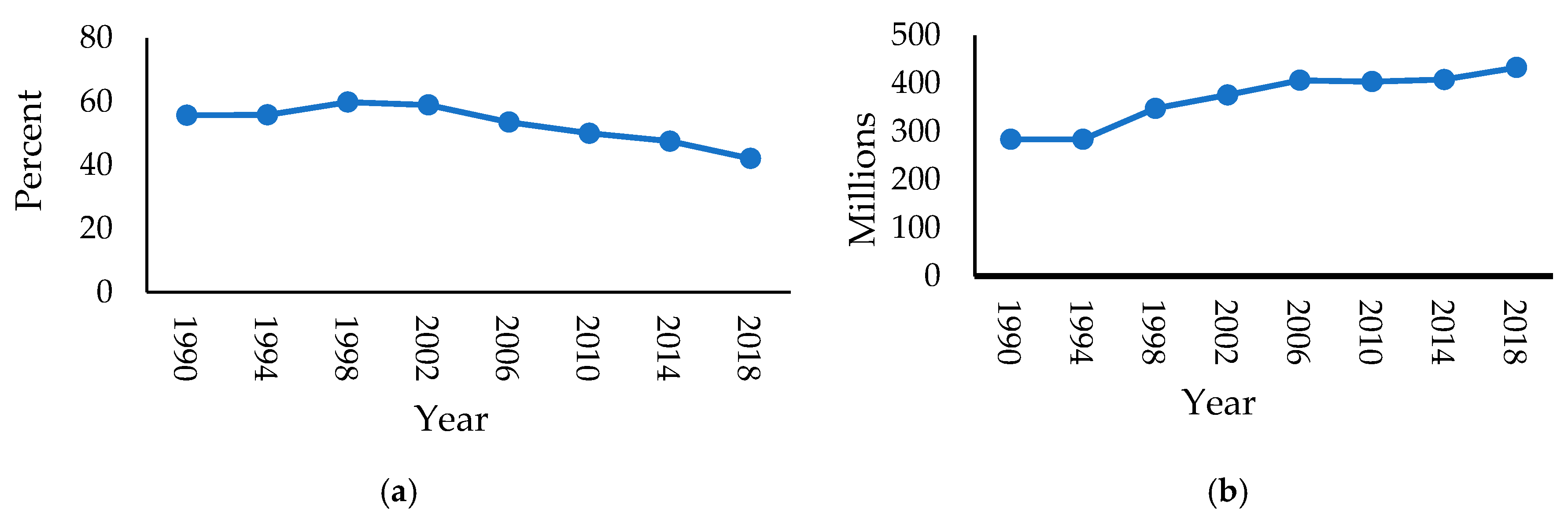
1.1.1. The Number of Poor and the Total Population in SSA

The international community’s attempts to achieve SDG 1 of zero poverty by 2030 have been disrupted by the global economic fallout from the COVID-19 pandemic. Africa is home to more than 70% of the world’s poor. Although poverty rates on the continent have been gradually increasing since the SDG period began (<1% in the previous two years), the number of people living in severe poverty in Africa was projected to increase by about 8% from 2019 to 2020 to nearly 520 million Africans. The poverty rates for 2018 matched the official World Bank poverty rates published by Povcalnet [20]. According to Wadjwa [2], the World Bank indicated that 1.9 billion people were living on less than $1.90 in 2015, from 736 million in 1990 (Figure 1). Statistics also display the number of people living on less than $1.90 per day increased by almost 1000 million, representing about a fifth of the population growth.

A good example can be seen from 1999 to 2014, when the number of poor people increased by just 30 million (Figure 1b). These statistics amounted to just 5% of the overall population growth in the area over the same period. As a result, poverty headcount rates have gradually declined since the mid-1990s, peaking at 60%. Despite this, poverty remained widespread, with nearly one in every two Africans living in poverty. Furthermore, poverty reduction has been extremely sluggish, averaging less than half a percentage point per year from 1999 to 2011 (See Figure 1a). Another report showed that the region’s poverty rate decreased by 1.6% between 2015 and 2018 (Figure 1b) [20].

Even though the rate of poverty in Sub-Saharan Africa (SSA) has not kept pace with population growth, poor people have continued to rise, with 413 million Africans living in extreme poverty in 2018, in comparison to 284 million in 1990. [21,22,23]. The progress done so far in reducing poverty in SSA has not been translated into equal rises in the demand above the US$3.20 mark. The slow development in Africa can also be seen at the country level, where the poverty rate in SSA barely narrowed between 1990 and 2018, ranging from the 0–80% point [22,23]. A report by Schoch and Lakner [23] states that 21 out of 45 African economies had a poverty headcount above 40% in 2018.

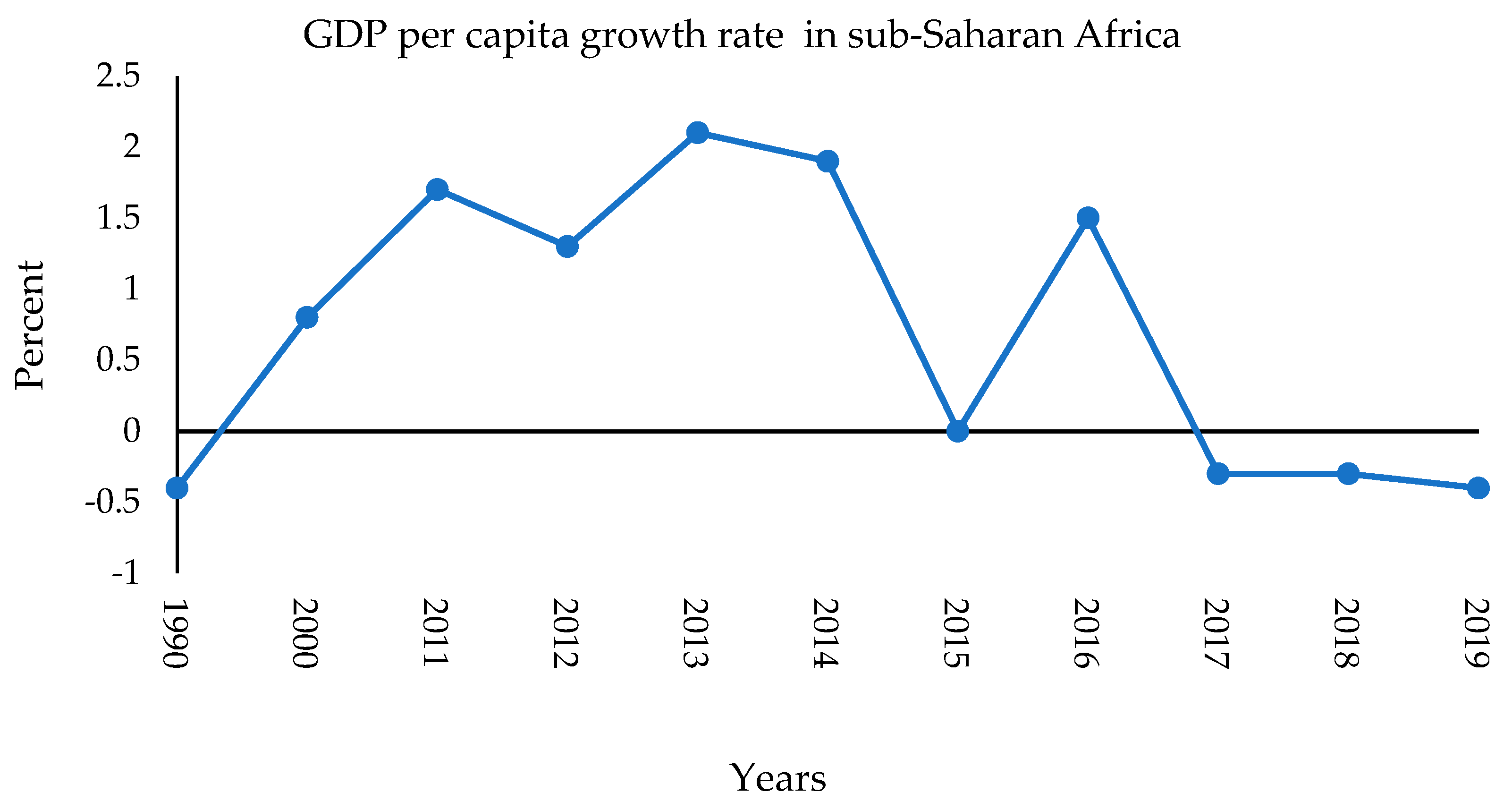
1.1.2. GDP Growth Rate per Capita

Africa was projected to recover in 2021 from its worst economic recession in half a century. Given the high rates of poverty still prevalent in many African countries, the sustainability of Africa’s growth rate in GDP per capita is essential. According to the African Development Bank Group [24], economic activity was constrained in 2020. Even after an unprecedented global pandemic caused by COVID-19, Africa’s economic growth was stifled. Africa’s real GDP will grow by 3.4% in 2021 after contracting by 2.1% in 2020.

Regardless of the proportion of Africans living in severe poverty, which had decreased from 57% to 43% (1990–2012), critical poverty problems still exist [2]. The number of people living in extreme poverty in African countries has increased by more than 100 million. In Africa’s conflict-affected nations, poverty reduction has been the slowest [25]. Maintaining an increase in growth rate in GDP per capita would be critical in reducing poverty levels in African countries. Poverty in Africa is widely regarded as a development problem. Different African countries experience diverse GDP per capita growth. In terms of how their growth rate in GDP per capita has risen, countries have differentiated themselves [25].

According to various studies, economic growth measured by real GDP per capita reduces poverty. Shorrocks and Van der Hoeven [26] pointed out that improved economic welfare in a country benefits all. Sachs [27] observed that the critical pro-poor development policy ensures that the country’s overall financial interest improves. Ulriksen [28] discovered that in selected developing countries in SSA, higher economic income levels, as calculated by growth rate in GDP per capita, are associated with lower poverty rates. These findings were consistent with that of Anyanwu and Erhijakpor [29] and Anyanwu and Ncube et al. [18] (Figure 2).

Government spending appears to play an essential role in poverty reduction, according to the literature. The premise is that government spending increases the standard of living in all aspects of society, especially for the poor. For example, according to the Keynesian perspective, government spending boosts aggregate demand, promoting economic growth and jobs, thus reducing poverty through the multiplier effect. Detailed discussion on the determinants or drivers of poverty has long been done by politicians, stakeholders, and other scholars. Recently, empirical research has emerged to support some of the most widely held theories about the causes of poverty [16]. A similar study has been done, providing a theoretical structure for understanding the causes of poverty. Poverty, they say, may be the product of domestic human problems [16].

1.1.3. Inequality and Gini Index

Inequality is the primary, most fundamental source of poverty. The poorest people in Africa are the most vulnerable. The COVID-19 crisis may intensify discontent among the most susceptible population if decisive action is not implemented. According to the Gini index, South Africa, currently, the most affected country in the SSA region, is among the world’s five most unequal nations. The virus’s initial impact on the world appears to have been primarily on the country’s wealthy, globally mobile community. Assume, however, that the virus is not controlled, and that population dissemination accelerates; in such cases, lower-income people who depend on public transit, do not have savings, and must continue working, cannot afford hygiene products, live in large families, or live in an informal settlement, may be particularly vulnerable [30]. One study has discovered a positive impact of inequality and wealth on poverty in Côte d’Ivoire at the regional level [31]. Another research study found that poverty was also more sensitive to income inequality than income [32]. Estimations done on the growth of elasticity in SSA countries indicated that the poverty growth elasticity is higher for communities with less inequality (lower Gini index). Naschold [33] used survey data from 1980 to 1998 to show that rising inequality leads to higher poverty levels for a given level of consumption. Another research, which looked for positive and meaningful Gini index coefficients for depth, poverty headcount, and severity indicators, found that a high level of inequality is linked to a higher level of poverty [29].

1.1.4. Education

As stated by the literature, education increases the stock of human capital, resulting in higher skills, labor productivity, and profits. Meanwhile, labor is the most valuable commodity for poor people; improving their education would help them escape poverty. Human capital investment is essential not only for economic development but also for poverty reduction [34]. It was found that rural households in India and Nigeria with a central earner who has not completed secondary school or only completed primary school were more likely to be poor than those with an immediate earner who has completed secondary school [35,36]. Higher education is not urgently needed in rural areas where only a few well-educated people live [37].

When it comes to poverty reduction, however, not all levels of education are created equal. It was shown that primary education is positively and substantially linked to the number of people living in poverty (poverty headcount) and that only in cases of individuals with at least a secondary education, which connects education and poverty, does poverty become negative and meaningful [17]. The poverty rate is positively correlated with basic literacy and primary education. Consistent with Botha’s results [38], there is a strong negative relationship between education and poverty in South Africa. His report suggested that low-education households are more likely to be disadvantaged than those with a higher level of education.

1.1.5. Lack of Essential Services and Agriculture

SSA has experienced its first setback in poverty reduction in two decades, threatening to undo all its progress toward the MDGs. Low-income families in both urban and rural areas were severely impacted. Considering the high level of informal urbanization in Africa, efforts to combat COVID-19 may have unintended consequences in developing countries, thereby putting more lives in danger than they intended to save [39]. The lack of essential housing services for the urban poor, especially water, increases the risk of disease outbreaks, particularly cholera and other similar diseases. Some urban poor people depend on informal employment to supplement their income and meet their basic needs, such as food [40]. If such individuals are forced to stay home—such as is the case during COVID-19 lockdowns—with little access to their primary source of income and no financial support from the government, the risk of starvation rises, further leading to food insecurity and potentially raising the risk of infection with other diseases [15]. Living in a particular region increases a person’s access to labor markets and centralized job opportunities. This is the case since the urban labor market offers a diverse range of employment, from manufacturing to services to clerical work. Due to the higher income produced by increased labor participation, increased urbanization is expected to reduce poverty rates [41]. While urbanization has the potential to minimize poverty, it also has the potential to increase it. Considering another study, backward linkages, agricultural productivity, remittance, rural and land process, rural non-farming employment, and consumer prices are the six main indirect channels by which urban population growth may affect rural poverty in surrounding areas [42]. It was also stated that urbanization has a significant impact on reducing rural poverty and the poverty of migrant peasants. As a result, the income or consumption difference between rural and urban areas was narrowed significantly [41]. In the labor market, urbanization plays a critical role. It has been pointed out that urbanization is linked to urban poverty [43]. The failure of the government’s anti-poverty policies in metropolitan cities has resulted in urbanization due to labor market rivalry between migrating peasants and urban workers [44].

1.1.6. Civil Wars, Conflicts, and Unemployment

Civil wars and conflicts have aggravated poverty by annihilating the economy’s beneficial powers (incredible human and physical capital), lowering social spending, disrupting economic activity due to an unsafe business climate, and raising transaction costs [43]. Because of the shortage of physical and human resources, relative prices of capital-intensive goods are increasing, whereas salaries and jobs for unskilled workers are falling. These factors contribute to poverty and a widening income gap, exacerbated as the number of war profiteers increases. As a result of the shortage of physical and human resources, relative prices of capital-intensive goods are increasing. More specifically, it has been postulated that violent conflict contributes to poverty, which in turn causes economic disruptions, such as:

• harm to infrastructure, institutions, and production [45];
• increased unemployment and inflation rates [46];
• wealth destruction; disintegration of community and social networks [47];
• changes of access to and relationship with local trade, housing credit, and insurance markets [48];
• forced displacement [49];
• a reduction in social-service spending; and
• a rise in the number of people who die or are injured [50].

1.1.7. Diseases

Although the African landmass is made up of countries with various foundations, health policies, and qualities, several factors—such as a young population, low urbanization rates, and comorbidities, such as HIV, anemia, and tuberculosis [51,52], as well as low urbanization rates—transcend these differences and have seldom been considered in the large number of studies published to date. For example, the epidemic’s death toll in African countries may be lower than elsewhere due to the median age of fewer than 20 years and low urbanization rates. However, a young population means that many infected people may not have shown symptoms, putting them at risk of infecting more people as is the case with symptomatic people [14]. As previously mentioned, the HIV/AIDS epidemic has had a significant impact on many countries in SSA. A considerable development threat causes the gross national product to rise slower, resulting in higher total health costs for both medical and social support. Studies have shown that the principal mechanisms by which HIV/AIDS can affect global poverty in Africa are the environmental effects [53]. Since the disease mainly affected people in are working-age group, the affected countries observed a drastic decline in their workforces, lowering the GDP growth rate unmistakably.

An experimental study on HIV in South Africa has shown that the incidence, severity, and depth are higher among households highly affected by the HIV/AIDS epidemic. In addition, members of such families are more likely to suffer from extreme poverty and income inconsistencies [54]. Additional evidence showed that the HIV outbreak reduced average income and raised poverty. Poverty is rising faster than anticipated, resulting in a decline in middle-income households [53].

2. Materials and Methods

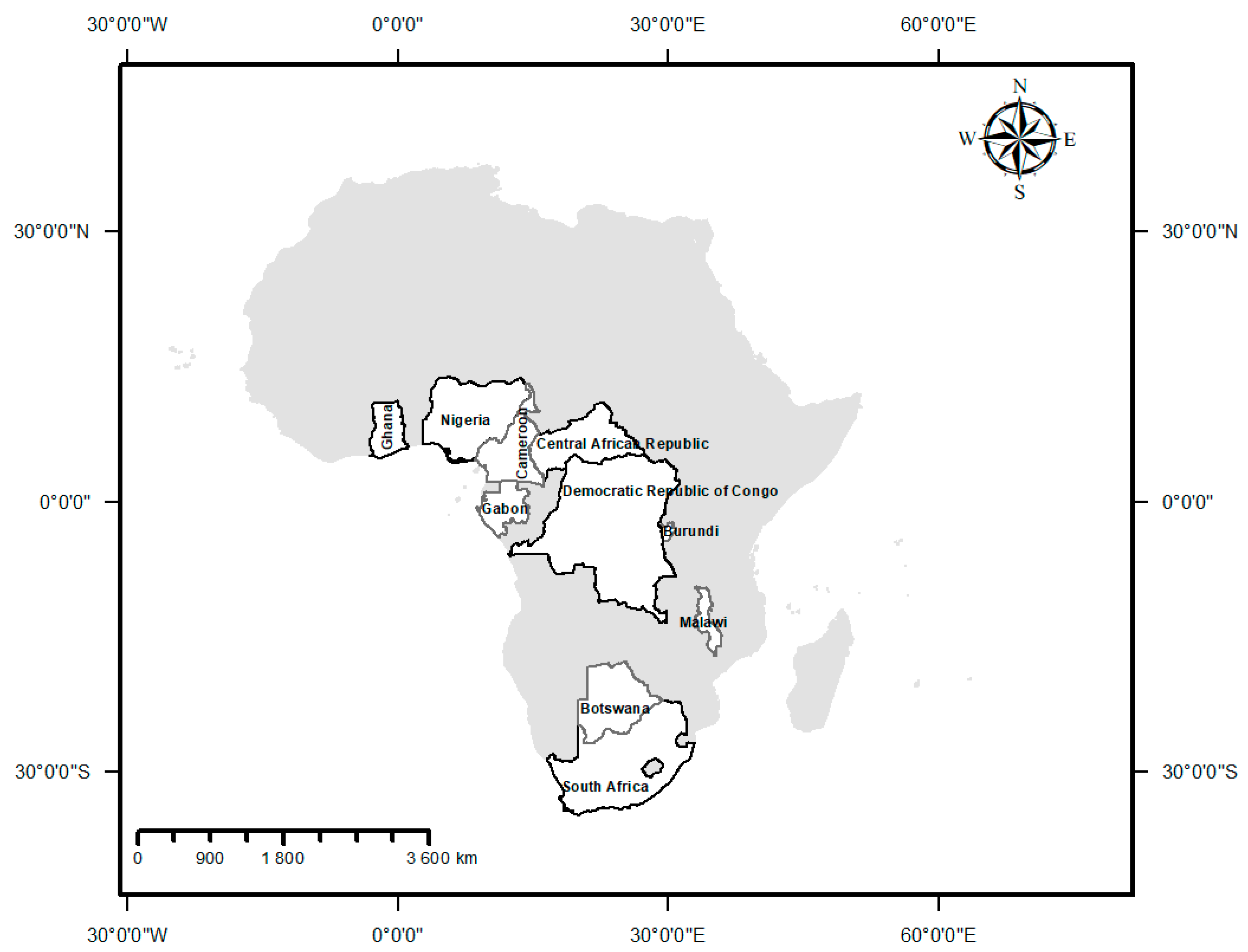
2.1. Description of the Study

SSA is made up of 52 African countries, including the island of Madagascar, but excludes northern Africa. The population of these countries living in severe poverty is rapidly increasing, with more than half of Central Africa living below the poverty line [55]. Therefore, ten selected countries from the regions were chosen for this study. These countries were obtained from South, Central, East, and West Africa; categories as upper-middle-income countries (Gabon, Botswana, South Africa), lower-middle-income countries (Cameroon, Ghana, Nigeria), low-income countries (Burundi, Central African Republic, Democratic Republic of the Congo, Malawi) were used in the study area. These countries are highlighted in yellow in Figure 3.

2.2. Selection of Variables

The analysis made use of five variables: per capita PCE (a proxy for poverty); Gini index; per capita income (a measure of inequality); GDP growth rate (measuring the economic growth rate and unemployment rate); and secondary school enrolment (both male and female). Poverty is the dependent variable; economic development and income inequality are the primary explanatory variables, while secondary school enrolments and unemployment are the control variables.

2.3. Data and Data Source

The study made use of the national representative poverty survey from 2015 to 2019. The database consisted of 10 selected countries in SSA, classified as usual upper-middle-income (Gabon, Botswana, South Africa), low-middle-income (Cameroon, Ghana, Nigeria), and low-income (Burundi, Central African Republic, the Democratic Republic of the Congo, Malawi) African countries.

The proxy for poverty is used as the dependent variable data obtained online from Povcalnet [20]. The World Population Prospects database provided the population info [56]. The World Bank’s development indicators [57] were the key data sources for the independent variables (explanatory and control). The variables, their descriptions, and their references are mentioned in

Table 1. Description of variables used.

Name of Variable	Code	Description	Sources
Per capita personal consumption expenditure	PCE	Proxy for poverty	Pocvalnet
Gross domestic product growth rate	GDP-GR	The GDP annual growth rate	World Bank, World Development Indicators [57]
Gross domestic product per capita (US$ 2010)	GDP-PC	GDP divided by the population	Done by authors
Secondary school enrolment rate	SSER	Ratio of children of official school age	Done by authors
Unemployment rate	UNEM	The percentage of the labor force that is unemployed but looking for jobs	Done by authors
Gini index	GI	Measures of income inequality	World Bank [57]
Population	P	Population in a country	United Nations, World Population Prospects [56]
Poverty rate	P(r)		Pocvalnet
Income group of the population susceptible	S(t)	Ratio of income below the poverty line
Upper middle-income population	PP(s)
Low-income population	PV(t)
Lower middle-income population	PM(t)
Population recovered from poverty	Λ

. Data were obtained from the World Bank’s online research tool called Povcalnet, published in 2020 by Washington, DC [20]. Yearly numbers of the total population and poverty rates from those countries were collected: for Ghana, data were collected from 1987 to 2020; for South Africa, data were collected from 1991 to 2020; and for Malawi, from 1997 to 2020. Yearly numbers of the total populations were multiplied by corresponding yearly numbers of poverty rates; the obtained results to represent the approximate numbers of actual numbers of poor people in each country are considered here. The difference in dates of the selected data is because data was not available for some countries for the same periods. A description of the parameters used is presented in Table 1 below.

2.4. Data Analysis

Data from 10 African countries, spanning five years from 2015 to 2019, were analyzed to understand the interacting dynamics of economic indicators on growth and poverty. While poverty rates had been slowly increasing on the continent since the beginning of SDGs, from 2019 to 2020, more than 70% of the global poverty was in African countries. Because of this, the countries were grouped into three different categories: low-income, low-middle-income, and lower upper-income groups respectively [57]. Using the per capita PCE growth rate as a proxy for poverty levels, the study compared the impact of growth, GDP, population size, and other variables on poverty, supposing that the general factors contributing to poverty have been substantially studied and researched. In this case, the literature still offered very little insight into comparative analyses of African countries at different levels of development and poverty. This study investigated countries at similar poverty levels within classification groups. It examined poverty dynamics within each group and between groups to recognize incidences and the impacts of variations on poverty in the economic variables at hand. Seven economic and sociopolitical variables were used in all the statistical analyses. A summary of the statistics of the variables is presented and examined. Tables of yearly average values per group; low, lower upper, and middle countries were also obtained for the variables PCE growth, GDP growth, GDP per capita, and total population (Supplementary Materials). All variables are correlated and regressed together to understand their co-monotonicity. The analysis was conducted using Microsoft Excel 2019 (perpetual License Tool Pak). Summary statistics of the variables with primary central locations and dispersion measures were obtained, presented, and examined.

2.4.1. Descriptive Statistics

The study used data from the World Bank [57] to examine the dynamics of economic indicators on growth and poverty in ten countries in the SSA region (categories: Upper-middle-income, low-middle-income, and low-income countries respectively.). Per capita (PCE) growth rate, GDP growth rate, secondary school enrolment GDP per capita, schooling, and the GINI index were all used in the descriptive analysis (see

Table 2. Descriptive statistics for independent variables.

Groups Statistics: Full Sample	Personal Consumption Expenditure Growth Rate	Gross Domestic Product Growth Rate	Gross Domestic Product Per Capita	Secondary School Enrolment	Total Population	GINI Index
Mean	0.50	1.81	3420.58	62.74	34,426,689.24	41.75
Standard deviation	4.52	3.59	3003.99	25.67	55,194,044.62	4.46
Minimum	−11.82	−10.19	525.48	12.72	2,007,882.00	35.10
Maximum	15.43	8.14	7446.25	99.63	200,963,599.00	44.70
Median	0.41	2.57	2230.32	70.14	14,137,941.50	43.60
Skewness	0.50	−1.21	0.60	−0.23	2.36	−1.92
Low-income countries	Personal consumption expenditure growth rate	Gross domestic product growth rate	Gross domestic product per capita	Secondary school enrolment	Total population	GINI index
Mean	0.84	0.44	597.47	62.37	9,559,240.35	44.70
Standard deviation	6.09	4.29	66.78	28.86	5,442,220.86	-
Minimum	−11.82	−10.19	525.48	12.72	4,493,170.00	-
Maximum	15.43	4.75	695.79	99.63	18,628,747.00	-
Median	0.05	2.16	590.04	71.37	7,770,269.00	-
Skewness	0.57	−1.05	0.70	−0.25	0.62	-
Low-middle-income countries	Personal consumption expenditure growth rate	Gross domestic product growth rate	Gross domestic product per capita	Secondary school enrolment	Total population	GINI index
Mean	−0.05	3.61	2252.77	67.88	81,555,361.80	39.30
Standard deviation	3.66	2.45	43.01	18.40	80,213,600.52	5.94
Minimum	−8.17	−1.62	2226.60	42.05	23,298,368.00	35.10
Maximum	6.99	8.14	2327.84	96.03	23,298,368.00	43.50
Median	0.63	3.55	2230.32	58.26	29,121,465.00	39.30
Skewness	−0.50	−0.17	1.99	0.07	0.80	-
Upper-middle-income countries	Personal consumption expenditure growth rate	Gross domestic product growth rate	Gross domestic productper capita	Secondary school enrolment	Total population	GINI index
Mean	0.60	1.83	7411.51	50.92	20,454,615.20	45.00
Standard deviation	2.70	2.84	31.48	28.62	26,750,359.47	7.73
Minimum	−6.47	−5.72	7362.41	28.10	2,007,882.00	38.00
Maximum	6.20	7.04	7446.25	90.54	58,558,270.00	53.30
Median	0.43	1.41	7413.61	35.87	2,254,067.00	43.70
Skewness	−0.62	−0.94	−0.95	0.79	0.79	-

).

2.4.2. Pearson Correlation and Regression Analysis

The strength of the relationship between parameters was estimated using the following scale: ±0.5 is large/strong, ±0.3 is medium/moderate, and ±0.1 is small/weak. The possible relationship between economic growth and poverty data is investigated using the Pearson correlation coefficients and a t-test using the Sigma Plot program (Microsoft Excel 365 Software version 11 for Windows). Significance was described as a p-value of less than 0.05. The Pearson correlation coefficient measures the degree of association between two variables and also how closely in theory they are related. The ordinary correlation matrix will specify the degree of multicollinearity between the variables under consideration before the measurement is performed (

Table 3. Pearson correlation of all the income groups (low, upper and lower middle income countries).

	Personal Consumption Expenditure	GDP Growth Rate	Per Capita GDP	UNEM	SSER	Ln (UNEM)	Ln (SSER)
Personal consumption expenditure	1
GDP growth rate	0.2902	1
Per capita GDP	0.3370	0.1938
UNEM	0.7041	−0.134	0.7548	1
SSER	−0.3605	−0.122	0.07266	0.0328	1
Ln (UNEM)	0.7743	−0.1261	0.5065	0.8835	−0.2114	1
Ln (SSER)	−0.3798	−0.1705	0.09158	0.0559	0.9964	−0.1767	1

 Large/strong relation ±0.5.  Medium/moderate and ±0.3.  Small/weak ±0.1. GDP = gross domestic product growth; GDP per capita (2010) (US$2010); SSER = secondary school enrolment for the low-income group; UNEM = unemployment rate, for the low-income, lower-middle-income and, upper-middle-income countries in SSA.

). The Statistical Package for Social Scientists (SPSS), version 20, was used to analyze the regression results. The average values of the independent variables (GDP per capita, unemployment, and secondary school enrolment rate) were taken from the Millennium Declaration year 2015–2019. The dependent variable –PCE growth rate—was regressed against covariates in three tentative models (

Table 4. Regression results on raw data for the best model suggested for low-income, lower-middle-income, and upper-middle-income sub-Saharan countries.

	Coefficients	Standard Error	t-Stat	p-Value	Lower 95%	Upper 95%	Lower 95%	Upper 95%
Intercept	19.83	23.99	0.8262	0.4325	−35.51	75.17	−35.51	75.17
GDP growth rate Low-income, upper and low-middle-income countries	0.4137	0.1953	2.117	0.06706	−0.0368	0.8643	−0.0368	0.8644
Ln (UNEM)	3.945	0.8500	4.641	0.001662	1.986	5.905	1.985	5.9059
Ln (SSER)	−5.999	5.715	−1.049	0.3245	−19.18	7.181	−19.17	7.1814

Multiple R = 0.88458; R² = 0.782482; Adjusted R² = 0.700913; Standard error = 2.362032; Observations = 12; F = 9.592871; S.F. = 0.005006.

), integrating the interactions between variables to establish the association between poverty and other independent variables similar to methodological stances in Adeyemi, Ijaiya and Raheem [19], Tsai [58] and Reddy [59] justifying PCE as dependent variable. Data values that were not usually distributed were transformed using the natural logarithm. The knowledge that was not traditionally distributed was converted using the natural logarithm. The critical determinant drivers of poverty in SSA were classified using a stepwise multivariate linear regression model based on country-level data for the 10 SSA countries. On the other hand, the regression study agreed that GDP growth does not always correspond to poverty reduction. Also included were two crucial economic growth factors that benefit the poor: secondary school enrolment and unemployment. They represent a new strategic doctrine of change in human capital growth that can be reflected in a broad spectrum of poverty levels across countries. Although higher educational levels are supposed to push poverty southward, the situation will deteriorate if unemployment rates continue to rise, ceteris paribus. The analysis was done in three sets of models, and the best model fit was considered (Equation (1)):

$$PCE G{R}_{it}={\beta }_0+{\beta }_1 GDP G{R}_{it}+{\beta }_2 \mathrm{L}n UNE{M}_{it}+{\beta }_3 \mathrm{L}n SSE{R}_{it}+{\epsilon }_{it}$$

(1)

where PCE GR is the growth rate of per capita PCE (a proxy for poverty rate);

GDP GR is the gross domestic product growth rate;

SSER (education) is the secondary school enrolment in its natural logarithm;

UNEM is the unemployment rate;

${\beta }_j$ (where j = 1…3) are parameters to be predictable;

L, countries, 1, 2, 3…. N;

t is the time = 1, 2 …T, and

$\epsilon$_it is the error term.

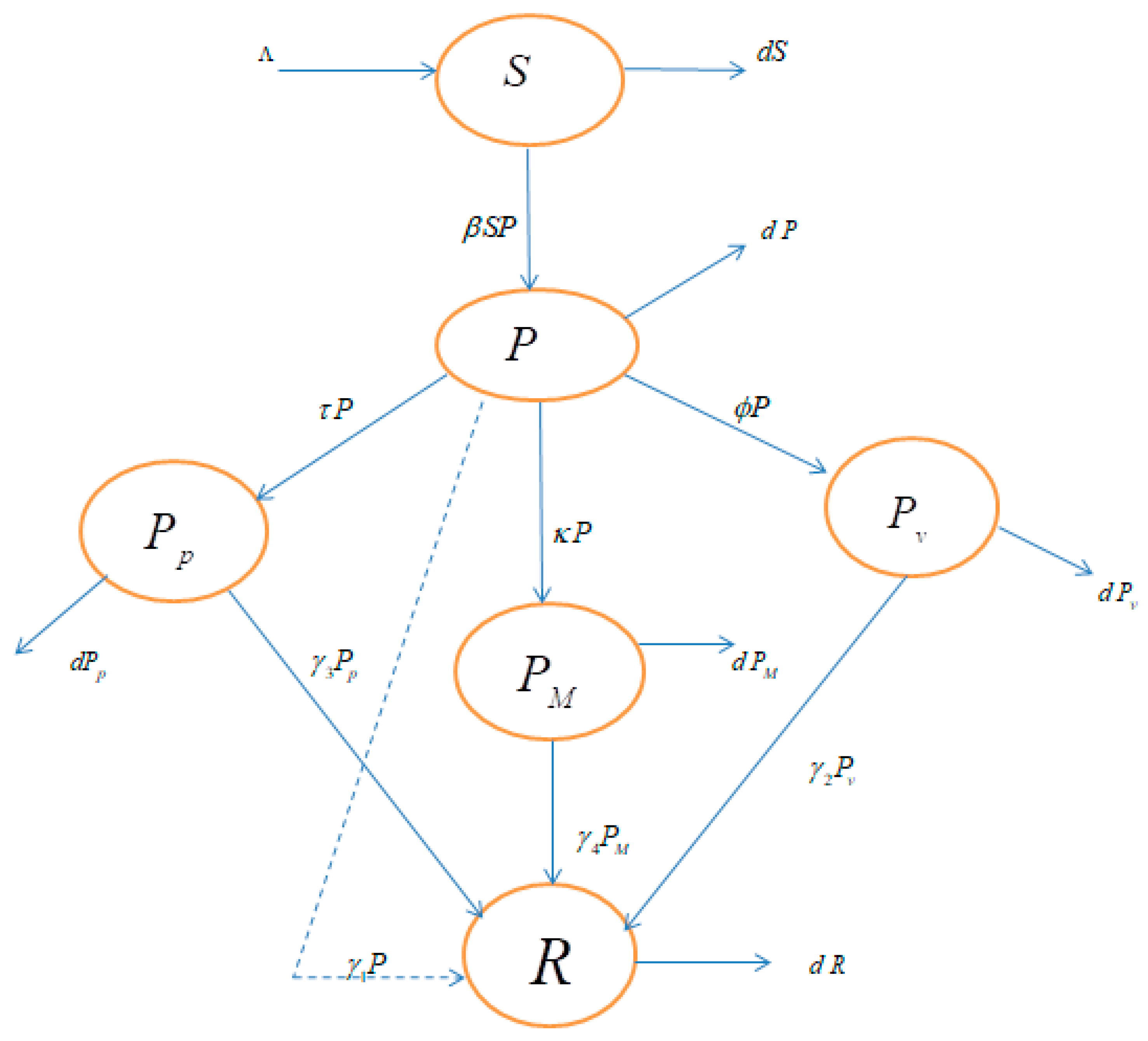
2.4.3. Theoretical Model Formulation

A deterministic compartmental modelling approach is used to design an income group of upper-middle, lower-middle, and low-income countries, individuals experiencing the impact of poverty in SSA countries. The ongoing COVID-19 pandemic has caused a sudden and sharp fall in the economy; this is expected to slow GDP per capita growth drastically. The number of poor individuals in the region is increasing day by day, leading to an increase in the level of poverty in SSA. It was presented as an income group the poor population in general; the upper-middle-income, low-middle-income, and low-income group respectively, was used. This section suggests a model that could explain the present situation and hint at a nearby future.

Let $N\left(t\right)$ denote the total population in the income groups, upper-middle-income, low-middle-income, and low-income countries respectively.

$S\left(t\right)$; people susceptible to becoming poor; $P_p\left(t\right)$ total population of people belonging to an income group; $P_v\left(t\right);$ people belonging to upper-middle-income countries, $P_M\left(t\right)$ people belonging to lower-middle-income countries, $R\left(t\right)$ a population recovered from poverty, and $\mathsf{\Lambda }$ is the recruiting rate. A possible model associated with this scenario is well explained in the following chart (Figure 4).

It is worth noting that this model has some limitations like all mathematical models; however, these models could help us have a hint of what could happen to understand nature under some restricted conditions.

From the above diagram, one can suggest a possible mathematical model that could be used to depict the dynamics of poverty within given settlements. The diagram explains that the rate of change of susceptible populations is equivalent to the recruitment minus the total number of susceptible dying naturally and those susceptible to joining the income groups. This can be converted to the following mathematical equation:

$$S^{\prime }\left(t\right)=\mathsf{\Lambda }-\beta S\left(t\right)P\left(t\right)-dS\left(t\right)$$

(2)

The rate of change of $P\left(t\right)$ concerning time is then equivalent to a proportion of susceptible individuals interacting with the income group of people susceptible to being poor, minus a proportion $\left(\varphi +\tau +\kappa +{\gamma }_1+d\right)P\left(t\right)$. The mathematical equation associated with this is given as:

$$P^{\prime }\left(t\right)=\beta S\left(t\right)P\left(t\right)-\left(\varphi +\tau +\kappa +{\gamma }_1+d\right)P\left(t\right)$$

(3)

The rate of change of people belonging to the upper-middle-income group $P_P\left(t\right)$ is equivalent to a proportion of $P\left(t\right), \tau P\left(t\right)$ minus a proportion of $P_P\left(t\right), \left({\gamma }_3+d\right)P_P\left(t\right)$, and the mathematical equation associate:

$$P_p^{\prime }\left(t\right)=\tau P\left(t\right)-\left({\gamma }_3+d\right)P_P\left(t\right)$$

(4)

The rate of change of people belonging to the lower-middle-income group $P_M\left(t\right)$ is equivalent to a proportion of $P\left(t\right),\kappa P\left(t\right)$ minus a proportion of $P_M\left(t\right),-\left({\gamma }_4+d\right)P_M\left(t\right)$, and the mathematical equation associate:

$$P_M^{\prime }\left(t\right)=\kappa P\left(t\right)-\left({\gamma }_4+d\right)P_M\left(t\right)$$

(5)

The rate of change of people belonging to the low-income group $v\left(t\right)$ is equivalent to a proportion of $P\left(t\right),\kappa P\left(t\right)$ minus a proportion of $P_v\left(t\right),-\left({\gamma }_3+d\right)P_v\left(t\right)$, and the mathematical equation associate:

$$P_v^{\prime }\left(t\right)=\varphi P\left(t\right)-\left({\gamma }_3+d\right)P_v\left(t\right)$$

(6)

The general system of equations associated with the described poverty dynamic can then be given as follows:

$$\left\{\begin{array}{c}{S}^{\prime }\left(t\right)=\mathsf{\Lambda }-\beta S\left(t\right)P\left(t\right)-dS\left(t\right)\hfill \\ P^{\prime }\left(t\right)=\beta S\left(t\right)P\left(t\right)-\left(\varphi +\tau +\kappa +{\gamma }_1+d\right)P\left(t\right)\hfill \\ P_p^{\prime }\left(t\right)=\tau P\left(t\right)-\left({\gamma }_3+d\right)P_P\left(t\right)\hfill \\ P_M^{\prime }\left(t\right)=\kappa P\left(t\right)-\left({\gamma }_4+d\right)P_M\left(t\right)\hfill \\ P_v^{\prime }\left(t\right)=\varphi P\left(t\right)-\left({\gamma }_3+d\right)P_v\left(t\right)\hfill \\ R^{\prime }\left(t\right)={\gamma }_{1}P\left(t\right)+{\gamma }_2{P}_v\left(t\right)+{\gamma }_3{P}_P\left(t\right)+{\gamma }_4{P}_M\left(t\right)-dR\left(t\right)\hfill \end{array}\right.$$

(7)

A basic reproductive number is denoted $R_0$. An expected number of cases, which reflect the size of the population here, are susceptible to being affected. The number is usually calculated using the next-generation matrix. For this model, an associate reproductive number was calculated as:

$$R_0=\frac{\beta \mathsf{\Lambda }}{d\left({\gamma }_1+d+\kappa +\tau +\varphi \right)}$$

(8)

• $\mathsf{\Lambda }$ is the recruitment rate (newborns, rich people that lost their wealth, and others);
• β rate of poverty;
• δ rate of low-income countries;
• τ rate of upper-middle-income countries;
• κ rate of lower-middle countries;
• γ₁, γ₂, γ₃, and γ₄ are rates at which income groups recover from poverty.

A numerical solution to the above system of equations is given as:

$$\left\{\begin{array}{c}\frac{S\left(t_{n+1}\right)-S\left(t_n\right)}{\Delta t}=\mathsf{\Lambda }-\beta S\left(t_n\right)P\left(t_n\right)-dS\left(t_n\right)\hfill \\ \frac{P\left(t_{n+1}\right)-P\left(t_n\right)}{\Delta t}=\beta S\left(t_n\right)P\left(t_n\right)-\left(\varphi +\tau +\kappa +{\gamma }_1+d\right)P\left(t_n\right)\hfill \\ \frac{P_P\left(t_{n+1}\right)-P_P\left(t_n\right)}{\Delta t}=\tau P\left(t_n\right)-\left({\gamma }_3+d\right)P_P\left(t_n\right)\hfill \\ \frac{P_M\left(t_{n+1}\right)-P_M\left(t_n\right)}{\Delta t}=\kappa P\left(t_n\right)-\left({\gamma }_4+d\right)P_M\left(t_n\right)\hfill \\ \frac{P_v\left(t_{n+1}\right)-P_v\left(t_n\right)}{\Delta t}=\varphi P\left(t_n\right)-\left({\gamma }_3+d\right)P_v\left(t_n\right)\hfill \\ \frac{R\left(t_{n+1}\right)-R\left(t_n\right)}{\Delta t}={\gamma }_{1}P\left(t_n\right)+{\gamma }_2{P}_v\left(t_n\right)+{\gamma }_3{P}_P\left(t_n\right)+{\gamma }_4{P}_M\left(t_n\right)-dR\left(t_n\right)\hfill \end{array}\right.$$

(9)

3. Results

3.1. Some Stylized Facts

Tables of yearly average values per group of upper-middle-income, low-middle-income, and low-income countries are obtained for the variables per capita PCE growth, GDP growth rate, GDP per capita, and total population. Excel line graphs with linear trend lines of the yearly average of groups for the variables per capita PCE growth and GDP growth rate is produced for the three groups, classified yearly. Comparative trend line graphs for each variable—per capita PCE growth rate and GDP growth rate—are also given on one plot for the three analysis groups’ low-income, low-middle-income, and upper-middle countries, respectively (Figure 5). Observing Figure 3, the PCE growth of upper-middle-income, low-middle-income, and low-income countries in SSA show that in 2016, the PCE growth rate of low-income countries (Burundi, Malawi, Democratic Republic of Congo, and the Central Africa Republic) was about 2.74% higher than that of upper-middle-income (South Africa, Gabon, and Botswana) countries, and double in the magnitude of that of lower-middle-income countries. (Cameroon, Ghana, and Nigeria).

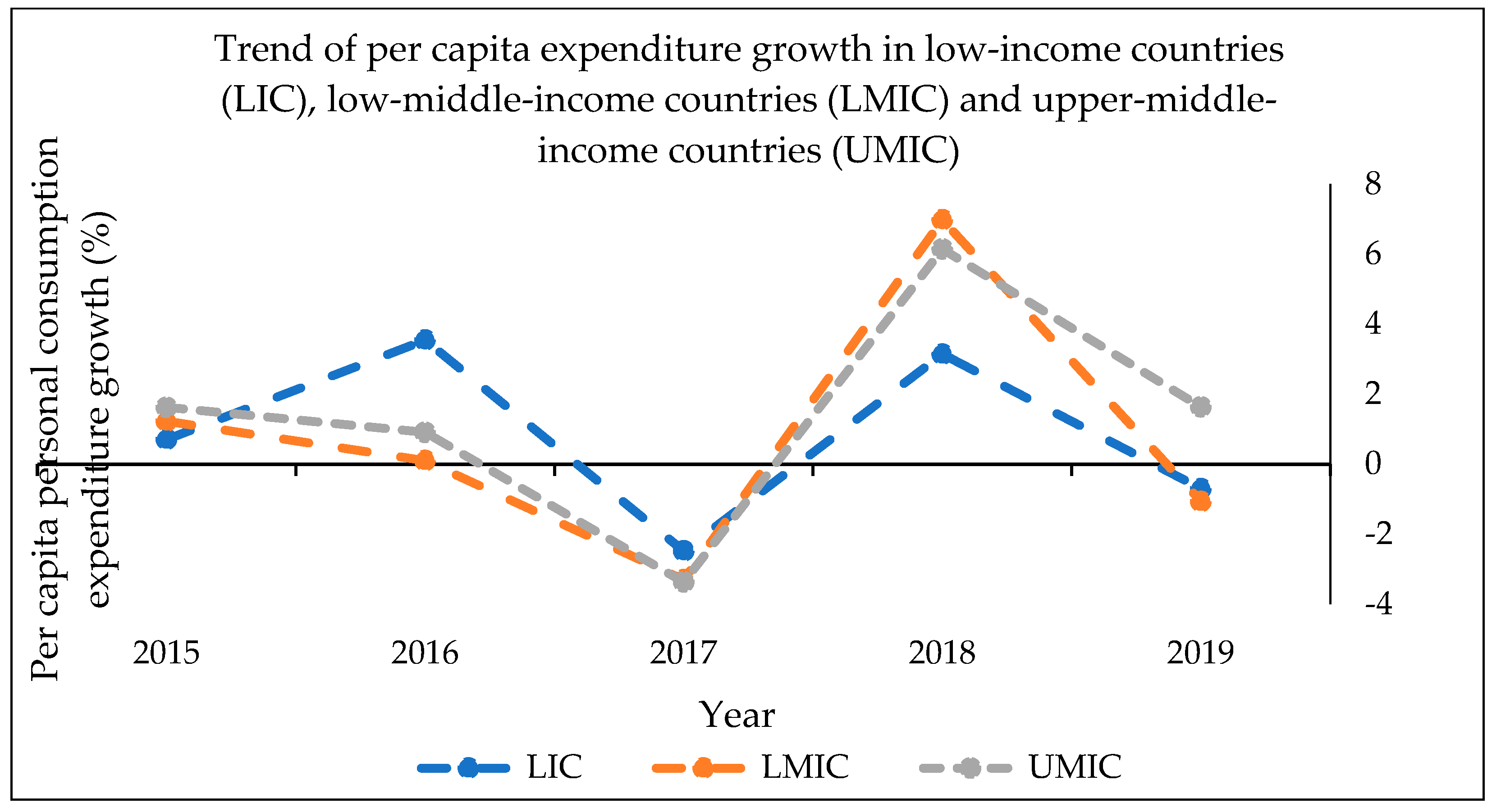
3.2. Per Capita Personal Consumption Expenditure Growth Rate

Furthermore, the PCE growth rates for low-income countries (Cameron, Ghana, and Nigeria) from 2015 to 2016 (0–3%) are curiously significantly higher than those of lower-middle-income countries (Malawi, Democratic Republic of Congo, Central Africa Republic, and Burundi) and upper-middle-income countries (South Africa, Gabon, and Botswana) that are trending negatively. Later from 2017 to 2018 (−7–4%) upper and lower-middle countries’ rates are significantly higher than those in low-income countries. Since poverty is described as a lack of consumption, and deprivation in the region, the per capita PCE of upper and lower-middle-income countries is supposed to be much higher than that of low-income countries. This is not always the case however, from 2015 to 2017 where low-income countries’ rates are higher than both lower and upper-middle-income countries respectively, implying that more households in the low-middle-income countries spend more on consumption than their African counterparts [60]. PCE as an indicator that shows less severe poverty in low-income countries than in lower and upper-middle-income countries, as seen in Figure 5, at least for the first portion of the graph.

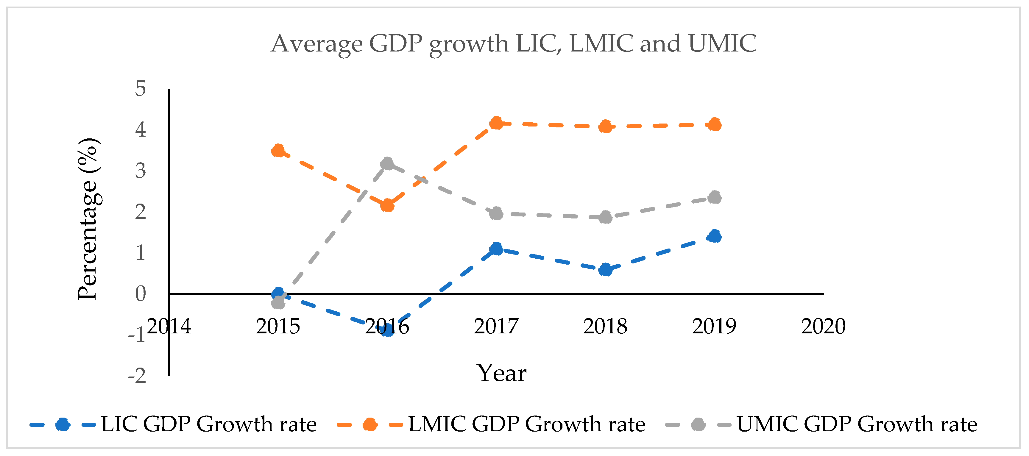
3.3. Average Annual GDP Growth

The annual GDP growth rate for upper-middle-income, low-middle-income, and low-income countries ranged from −1% to 5% per year from 2015 to 2019. Between 2015 and 2016, the average GDP growth dropped from 3.18% to −0.89% for low-income countries, from 3.5% to 2.16% for lower-middle-income countries, while it grew from −0.21% to 2.18% for upper-middle-income countries. From 2016 to 2019, both low-income and lower-middle-income countries recorded GDP growth rate increases, in ranges of −0.89% to 1.41% and 2.16% to 4.14%, respectively. In the same period, upper-middle-income countries suffered successive drops in growth rates from 3.18% to 1.96% to 1.87% in 2016, 2017, and 2018 respectively, before recording an increase from 1.87% to 2.36% in 2019 (see Figure 6).

Comparing the PCE growth-rate line graphs (Figure 5) and the GDP growth-rate line graphs (Figure 6) for the three groups of countries classified, we notice that the period of PCE growth (blue line low-income countries (2015–2016) and (2017–2018)) (Figure 5) translates to decreasing GDP growth rate (blue line (2015–2016) and (2017–2018)) (Figure 6). For the first half of the period studied (2015–2017), the PCE growth-rate line graph (Figure 5) shows lower poverty levels in low, lower, and upper-middle-income countries respectively. In contrast, the GDP growth rate line graph (Figure 6) indicates almost systematically contradicting growth dynamics with PCE in all three categories of low, upper, and lower-middle countries. On average, over the first half of the period, the PCE growth line hints at a lower poverty level for the low-income countries than the recorded level for upper-middle-income countries. As pointed out in the introductory descriptive analysis, Malawi, belonging to low-income countries, recorded the sample minimum PCE growth value in 2016. Although this low value impacts the PCE growth rate of the LI countries, the suggestion made in Figure 5 and Figure 6, that poverty levels could be higher where growth measures are higher, underlines the importance of social inequalities and wealth distribution in the analysis of poverty. A small group may concentrate the majority of the wealth created. Aggregate values growth and per capita growth values will be higher, whereas the intensity of poverty may also be accentuated paradoxically. For the second half of the study period (2017–2019), Figure 5 and Figure 6 portray the somewhat anticipated ordinal relationships between the groups. Higher PCE growth values and higher GDP growth correspond to lower and upper-middle-income and low-income countries respectively. An exception is observed for GDP growth rate values. The lower-middle-income group has a slightly larger value (last quarter of 2017) than the value for the upper-middle-income countries group. The PCE growth is substantially more significant for the upper-middle-income group. If needs be, this can only be seen as a reminder that growth does not mean less poverty, and inequality among other parameters, and factored in that scenario.

3.4. Variation of Poverty and Economic Growth Variables

The study used a total of 12 observations with average mean, standard deviation, median, and skewness variables, as shown in Table 2. For the response variable per capita PCE increase, the standard deviations mean value rises to 6.0. Over the period considered, the average PCE growth is lower in middle-income countries (−0.05) than it is in low-income countries (0.84). However, as expected, GDP growth rate and GDP per capita increased in the categories; of low-income, lower and upper-middle-income countries, respectively. A similar stance is achieved when comparing tables of yearly averages for PCE growth, and GDP growth for low and middle-income countries respectively. Most of the descriptive table variables have a positive skewness, except the GDP growth in all three categorized countries. The full sample for PCE growth is right-skewed (0.4), while its GDP growth is left-skewed (−1.01), indicating that poverty can move in the opposite direction, despite a positive growth rate. The same can be observed for the two variables, PCE growth and GDP growth in the country groups low-income and upper-middle-income countries. For lower-middle-income groups, and countries, both indicators are left-skewed.

3.5. Determinants of Economic Factors and Poverty in SSA

The Pearson correlation coefficients for the variables used in the model are shown in Table 3. The dependent variable is PCE growth, which is used as a proxy for the poverty level. All variables are correlated together to understand their co-monotonicity. The overall sample indicates a lot of data dispersion across almost all of the variables of interest. As far as correlation and analysis are concerned, GDP growth is negatively correlated with GDP per capita, secondary school enrolment, unemployment, the natural logarithm of unemployment (Ln UNEM), the natural logarithm of secondary school enrolment (Ln SSER), and has a weak positive correlation with PCE growth (29%). The finding asserts what has been postulated earlier that the incidence and impact of upward trending growth on poverty reduction are not always positive. It is worth remembering that the observed interactions are not enough to draw any conclusions about the regressors on the outcome variable. The best model,$PCE GR={\beta }_0+{\beta }_{1}GDP GR+{\beta }_2 \mathrm{L}n UNEM+{\beta }_3 \mathrm{L}n SCER+\epsilon$ has an r² = 78%. The results obtained are presented in Table 4. The model indicates that 78% of variations in poverty can be accounted for by the model. That is, for the ten countries in the study sample, the logarithmic unemployment rate appears to have the most significant contribution to poverty. The Pearson correlation coefficient shows that a positive correlation exists between the poverty (PCE growth) logarithmic and unemployment rate Ln (UNEM) (77%). Ln (UNEM) is the only significant covariate in the model (p 0.05% level). The best model shows a strong association between poverty and unemployment rates (logarithmic scale) (p = 0.001662). The incidence and impact of the unemployment rate on poverty are positive. GDP growth rate becomes significant at 10% level, p is 0.067. The regression analysis sometimes agrees that GDP growth does not always move in agreement with poverty elimination.

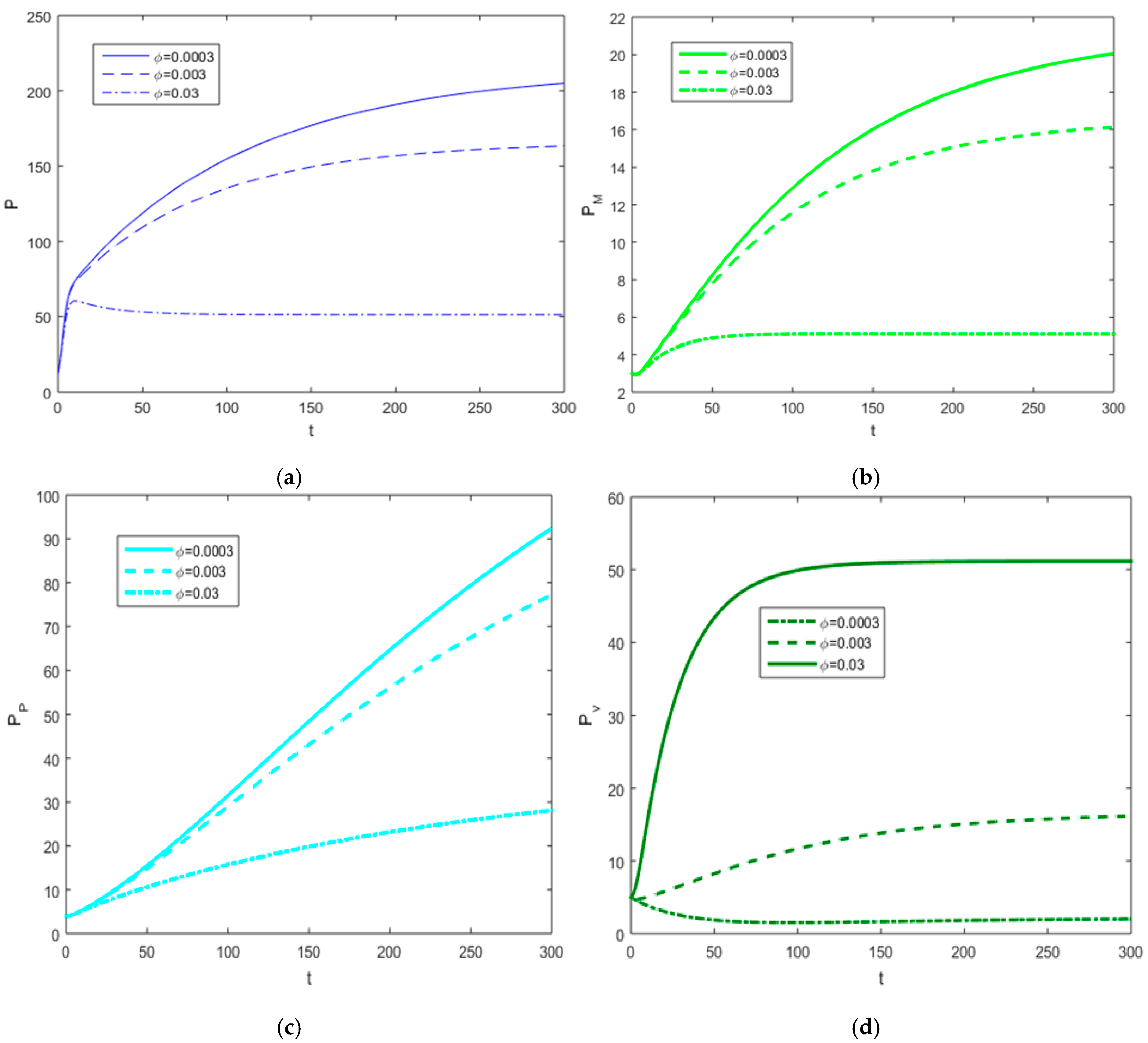
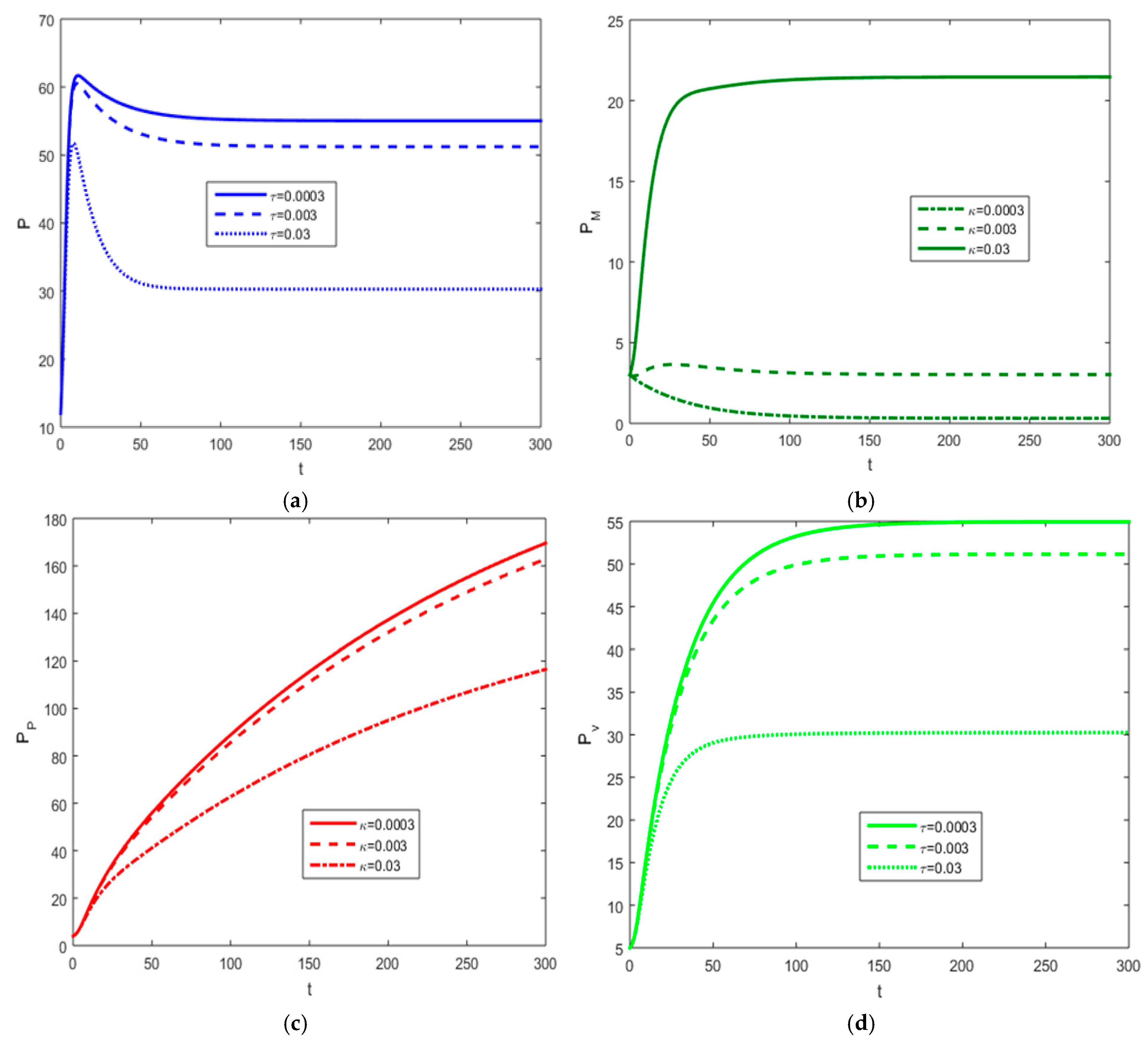
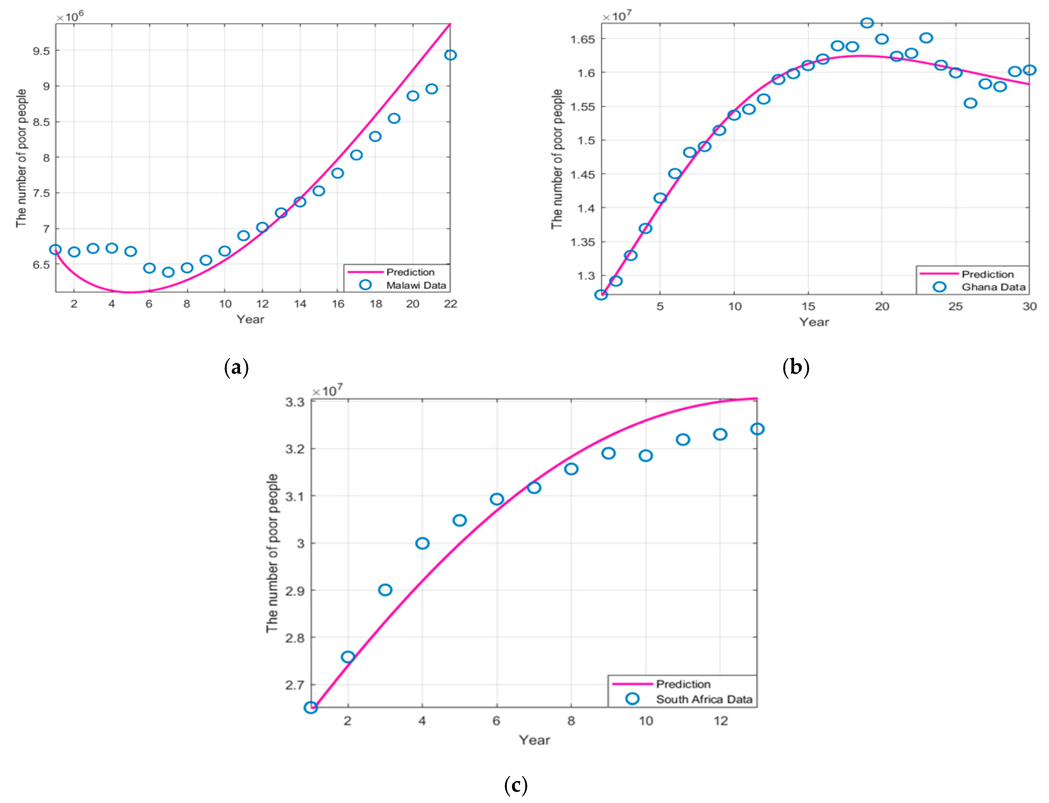
3.6. Poverty Model in Sub-Saharan Africa

By using a mathematical program, MATLAB 2019, plots of poverty rates versus the average leap year of three selected countries each from the different income groups: upper-middle-income (South Africa), low-middle-income (Ghana), and low-income (Malawi) countries were done. The sudden fall in GDP per capita has led to a drastic fall in the economy, thereby causing poverty in the selected countries to rise since 2019. These countries were then selected for this poverty model. A mathematical system of the equation was derived from Equations (2)–(6) above. The numerical solution results obtained are depicted in Figure 7 and Figure 8. To achieve the predicted model stimulated, the following parameters were considered:

$$\lambda =0.2, \beta =0.01, d=\frac{1}{70\times 365}, \varphi =0.03, \tau =0.03, \kappa =0.03, {\gamma }_1=0.003, {\gamma }_2=0.03,{\gamma }_3=0.004 , {\gamma }_4=0.03$$

(10)

Equations (2) to (6) indicate the sensitivity of poverty rates, including ϕ, τ, and $\kappa$ for different countries in the upper-middle-income population, and the outcome results are presented (Figure 7 and Figure 8), which were compared to the suggested mathematical model as presented in Figure 9 below. The initial conditions used to perform the numerical solution of the mathematical equation are the initial numbers of the poor population for these three countries. They were then obtained in 1987, 1988, and 1993 for Ghana, Malawi, and South Africa. These poverty rates contributed to the unemployment rate, illiteracy rate, and other factors contributing to poverty in a given country from either upper-middle-income, low-middle-income, or low-income (Figure 8).

To appreciate the efficiency of the suggested theoretical model, data were collected from three different countries, including South Africa, Ghana, and Malawi, chosen from categories of upper and lower-middle-income countries, respectively. Numerical solutions from the model were compared with collected data as presented in Figure 9a–c.

4. Discussion

The study investigated the critical determinant of poverty based on economic indicators and growth during the year 2015–2019. A total of seven variables were analyzed: GDP growth rate, per capita PCE growth, GDP per capita, unemployment rate, secondary school enrolment, total population, and GINI index. The PCE growth was used as a proxy for poverty level, and GDP growth average value and standard deviation value showed an increasing strength (−0.05–6%) for upper and lower-middle-income countries, and low-income countries in SSA respectively. This means that variable values are far apart from one country to another, justifying the approach of regrouping countries of similar socio-economic status for the analysis. Per capita PCE growth showed the highest mean value (3.66) in lower-middle-income countries, followed by 0.84 in low-middle-income countries. The lowest mean value (−0.05) was obtained for the lower-middle-income countries. The higher the PCE growth rate value, the less poverty, and equivalently, the lower the PCE growth rate value, the more acute is poverty. For the total sample, the median PCE growth rate is 0.63%, the minimum value is −11.82%, and the maximum is 15.43%. It is expected that the value indicating the most extreme level of poverty comes from low-income countries. However, it is an intriguing fact that the maximum PCE growth rate values come from the same group of low-income countries (Malawi).

This speaks to the intricacy of the tandem growth inequality and its incidence of poverty. That Malawi recorded in 2016 the best value indicative of minimal poverty, better than countries in the lower and upper-middle-income groups, also highlights the necessity of a broader perspective integrating various measures and their co-monotonicity, rather than single action-focused analyses.

Economic Indicators, Regression Model, and Its Impacts on Poverty

Looking at the GDP growth rate, the mean values increased from 0.44 to 1.83 to 3.61 for low-income to upper-middle-income to lower-middle-income countries. This is an early suggestion from summary statistics that growth does not always translate to poverty reduction. Considering their skewed behavior, the GDP growth rate and per capita PCE displayed high positively, moderately, and weakly skewed behavior with minor significant changes in their standard deviation (upper-middle-income to low-income countries respectively). This implies that the standard deviation showed a minimum dispersion from the mean. This result agrees with a comparable study done in SSA when verifying whether economic growth reduces the incidence of poverty. For lower-middle-income countries such as Nigeria, the average mean value (<1) and standard deviation value (<0.1) were obtained for the per capita PCE growth. The highest mean value obtained for their GDP economic growth rate was 0.43, with a standard deviation of 4.3 acquired, which was widely distributed from the sample mean [61].

The relationship among the various economic indicator parameters, the PCE growth rate, unemployment, and secondary school enrolment (Table 3) showed a strong positive (>0.51), moderate (>0.34), and weak (>0.1) correlation. GDP per capita correlates moderately and weak with PCE growth and GDP growth. Unemployment showed a solid and weak correlation with PCE growth, GDP per capita, and GDP growth respectively. Secondary school enrolment showed a moderate, very weak correlation with per capita PCE, unemployment rate, and GDP growth. The result confirms what has previously been hypothesized: the incidence and effect of upward trending growth on poverty reduction are not always optimistic. GDP growth has a weak positive correlation with PCE growth but is negatively correlated with GDP per capita, secondary school enrolment, unemployment, and Ln (SSER) (r = 0.29%). Economic growth, per capita income, education, and unemployment all had a positive relationship with PCE growth, but the correlations were low (r = 0.75%) [61]. Since all the correlation coefficients were less than 0.99, there is little evidence of more explanatory variables among the regressors in the model.

The outcome from the three models depicted the dependent variable for poverty (PCE) growth rate that was regressed against the GDP growth rate, unemployment, and secondary school enrolment. The best model (Equation (11)) shows that unemployment is strongly associated with poverty at a 5% significant level (p = 0.001662). The model has an R² of 78%, indicating that 78% of variations in poverty can be accounted for by the following variables of the model, GDP growth rate, Ln unemployment rate, and Ln secondary school enrolment rate.

According to the MDGs, GDP growth and secondary school enrolment (education) showed a weak association in eliminating poverty in SSA (SDG 1).

$$PCEG{R}_{it}={\beta }_0+{\beta }_1 GDP G{R}_{it}+{\beta }_2 \mathrm{L}n UNE{M}_{it}+{\beta }_3 \mathrm{L}n SSE{R}_{it}+{\epsilon }_{it}$$

(11)

Given that, per capita, PCE is a reliable predictor of poverty, this finding explains how economic growth and the unemployment rate can increase an individual’s consumption ability to meet their needs, thus reducing poverty. This result is consistent in a situation where upper-middle-income lower-middle-income countries’ economic growth is reducing poverty (high- and middle-income earners), suggesting that economic growth increases consumption expenditure (>4%) [7,62,63,64].

The GDP growth–PCE growth rate (poverty) relationship showed a simple pattern: The coefficient is not always positive for all specifications; it is not always statistically significant for lower-middle-income, low-income, and lower-middle-income countries (upper to lower-income, and low-income group respectively). Although positive in three specifications, the coefficient of the GDP growth rate is only significant at 10% and 29% levels for specific low-income and lower-middle-income countries. (p = 0.00671, 0.256). At a 5% level, GDP growth is not significant. This implies more than a 6% increase in consumer spending on average, ceteris paribus. Individuals can increase consumption as their income increases, so this outcome is predicted and predictable. According to the interpretation, unequal income distribution in these countries may worsen poverty by close to 30%. This fact showed how poverty is exacerbated by inequality. According to the findings, poverty may be more aggravated by income inequality than income.

In the education sector from the suggested model, the regression results showed that the secondary school enrolment rate does not play a significant role in poverty variations. The p-value is 0.33. Although intuitive knowledge may suggest otherwise, this result may be due to various reasons about the sample size and missing data values. A total of 40–50% of the values of secondary school enrolment in developing countries were non-existent for the period under analysis. These results are consistent with the results from the literature studies by Anyanwu [17] and Tilak [65]. They explained that not all levels of education are created equal when it comes to poverty reduction. Primary education is positively and substantially linked to the number of people living in poverty. Pure literacy and primary education are correlated with poverty. Another researcher found similar results, with a clear negative relationship between education and poverty in South Africa. Households with a low level of education are more likely to be poor than those with a higher level of education [38].

In contrast to the above, studies have shown that schooling increases earnings reasonably linearly, with each additional year of primary education contributing about 8% to a child’s earnings. Income would increase by about 50% over the average six years of primary schooling. These gains are especially notable in upper-middle-income, lower-middle-income, and low-income countries, with the highest out-of-school rates of all ages accounting for 33 million of the world’s 61 million out-of-school children [66]. Education has also helped to decrease poverty, especially in the time before the COVID-19 pandemic. Africa is one of the continents whose educational systems have been particularly affected by the deadly pandemic. More than 98% of teaching and learning in these continents was incompatible with the country-wide lockdown. In the shutting down of schools across upper and lower-middle-income and low-income countries in SSA, over 91% of them are primary and secondary school learners.

Apart from pharmaceutical treatments and other prevention measures such as wearing a face mask and washing hands, social distancing has proven to be the most effective way of limiting the spread of COVID-19. The practical implementation of social distancing demands that schools be closed for as long as each government from different countries is confident that the pandemic has been curtailed enough for the safety of learners and teachers before recommencing back to the classroom. In low- and middle-income nations, about half a percentage of 10-year-old children had either struggled to learn to read with comprehension or had dropped out entirely. The World Bank refers to “learning poverty” [66].

School closures due to COVID-19, in the most damaging cases, may exacerbate the learning deficit gap. SSA (low- and middle-income nations) continued to have the highest number of children unable to read (about 2%). Schools are missing extended periods of learning due to disease outbreaks that may have both a chronological and a long-lasting effect on the educational system [67]. The temporal damage includes curriculum interruption, which may take a long time to recover, and the undeviating spoil, which consists of the possibility that students will never return to school after the virus outbreak has ended, because of the concerns of COVID-19 inhibition in SSA. It is possible that social distancing would be applied over a more extended period than predicted. According to Davies et al. [68], the South African Department of Education has proposed a gradual reopening of schools, dubbed the “Phasing in Approach”. Countries worldwide have been experimenting with phasing in to see if they can open schools across SSA. According to Akinpelu [69], about 60% of Nigerians (a West African country) do not have access to the internet. Cell phone data, which could also be used as a learning intermediate, is more encouraging. According to the survey, 169.2 million Nigerians, or 83% of the population, have access to cell phone connections; however, half of these, or 84.5 million people, live in rural areas [69].

Moreover, unemployment (logarithm scale), is reducing poverty (p = 0.001662), for all country’s categories (upper and low-middle-income and low-income countries) (70–77%). The COVID-19 could translate into higher unemployment since tourism and related services are likely to experience cutbacks [70]. The provision of unemployment benefits, which temporarily alleviates hardship, is the possible reason for such outcomes. The variance in the outcome variable described by the regressors is shown by the R-squared, which ranged from 5–70%. Finally, except for the normal flawed country study, the statistically significant F-statistic confirms that the regressors were jointly substantial in explaining per capita PCE growth.

The spread of the global COVID-19 pandemic has placed a hard stroke on the African content. In countries such as Nigeria, the COVID-19 shocks have fallen harder in urban areas where the initial effects of the lockdowns have been felt more strongly. Low-wage and casual workers who work in jobs that cannot be done from home, such as retail, distribution, and hospitality, have suffered the most significant income losses. According to a telephonic survey conducted in the SSA countries mentioned earlier, jobs have been lost, businesses have closed, and markets have been disrupted due to the lockdowns [15,70]. Countries all over the world have used strict lockdowns to try to stop the spread of the COVID-19 pandemic. However, in most developed countries in SSA, especially in developing world cities, this approach is challenging to implement. Lockdowns are more likely to cause problems for the urban poor due to unemployment.

The PCE growth rate (poverty) and the unemployment rate have shown a sharp increase in developed and emerging markets and developing economies in SSA countries. However, there are some challenges in meeting unemployment and poverty in upper and low-middle-income and low-income countries in SSA regarding the suggested model.

Initially, the growth rate is insufficient. In achieving the MDG 1 of halving the number of poor people by 2030, the growth rate of African countries would need to rise at a rate of about 7% per year. This growth rate is substantially higher than the previous decade’s average, about <4% (2019–2021). The second issue is low labor absorption in the development sectors. However, most progress has been made in the traditionally capital-intensive extractive industry. Agriculture, which employs the most people from African countries, has experienced low productivity growth, resulting in a lack of actual employment and income security for the people, particularly in rural areas. Moreover, economic prosperity has resulted in inequity in the distribution of opportunities [61]. Poor people cannot contribute meaningfully to the economy as either goods and service producers or labor providers. Since the 1980s, there has been a strong link between job performance and poverty prevalence; poverty rates have remained roughly constant in lockstep with the observed unemployment rate [71]. And the poor’s vulnerability has been exacerbated by the instability of development. Just a few African countries have been able to maintain growth over time. Yet, increasing jobs and minimizing poverty are precisely what is needed in achieving the goal.

When looking at the theoretical modelling section, data was collected from three different countries, South Africa, Ghana, and Malawi, chosen from categories of upper-middle, lower-middle, and low-income countries respectively. Their simulation results (Figure 9) were compared with suggested mathematical models (Figure 7 and Figure 8). From these results, one can see in the case of a lower-income country (Malawi), that the rate of poverty has increased significantly from 1997 to 2004; with approximately 97.1% of Malawians living in poverty, according to the threshold headcount ratio at $5.50 a day (Figure 9a). The country observed an insignificant decline in the poverty rate from 2004 to 2010, ranging from 97.1% to 96.3%. Again, from 2010 to date, the rate of poverty in Malawi was increasing. In particular, due to the breakout of COVID-19 and the measure put in place to help flatten the curve of this deadly disease, the country has observed a significant increase in the poverty rate. The mathematical model suggests that Malawi may have a poorer population than the presented rates in the last three years. There is a significant decline in the poverty rate compared to lower-middle-income countries such as Ghana, especially from 1987 to 1988 (Figure 9b). The country has observed a slight decline of −1.20 % of the poor population; however, from 1988 to 1991, the poverty rate has slightly increased from approximately 90% to 92.3%. Serious efforts have been made in this country from 1993 to date as the poverty rate has significantly declined from 93% to 56.3%. Of course, it can be argued that more than half of the population of Ghana are still living under poor conditions, compared to many Western countries where less than 3% of the total population lives under poor conditions—for example, a country such as Belarus, where the poverty rate decreased from 76.9% in 1998 to 0.4% in 2018.

In the last year, unfortunately, due to the impact of COVID-19, the country has also observed a slight increase in the poverty rate. From 1993 to 1996, a normal developing country such as South Africa has witnessed a 4.10% increase in poor populations, corresponding to abolishing the apartheid regime (Figure 9c). From 1996 to 2010, the poverty rate was reduced from 71% to 56%; however, from 2011 to date, there is a slighter increase in the poverty rate. More precisely, in the last two years, unemployment has increased significantly due to the spread of COVID-19, affecting the poverty rate. In general, some efforts have been made to reduce poverty in SSA countries. Looking at the data, it is clear that more than half of individuals living in these different countries are poor. The sensitivity analysis of the poverty rate shows that reducing the unemployment rate in these different countries will reduce poverty. These results are in good agreement with those of the regression analysis, where it was also shown that high unemployment results in a high rate of poverty.

Relating the poverty model scenario to the economic indicators (GDP, growth, GDP per capita, education enrolment, and unemployment), poverty has impacted in one way or another economy. Looking at upper-middle-income the model suggested with the ongoing COVID-19 pandemic, that poverty was projected to rise to close to 50% from 2019 to 2020. Poverty reduction has been achieved through broad-based economic growth since 2017. The number of people living in poverty has risen due to the increasing population and urbanization of the usual upper-income group. In contrast, there is a decrease in the rural cities. It has been shown that urban households provide fewer economic opportunities to improve their income levels and obtain adequate living standards. Also, the rate of in-immigration has increased in recent years [70]. South Africa is one of the upper-middle-income countries where inequality is high and persistent and has increased since 1994. The number of COVID-19 positive cases is rising and is likely to have a devastating effect on the economic consequences of the country, which has already devastated the economy. Many individuals have lost their jobs. Consequently, the rate of poverty is increasing in the country, leading many individuals to unemployed.

However, middle-income countries portrayed in the hypothetical model have experienced increments in Cameroon and Nigeria and decreased in Ghana the rate of poverty from 2012 to 2019. Nonetheless, there has been a slight expansion in the destitution rate in the helpless lower-middle-income country such as Ghana by 13.3% in 2016. This new pandemic spread has likewise added to the increase in the neediness rate in the center (low-income group). Concerning the financial-economic standpoint in lower-middle countries (Nigeria), the global money-related asset proclaims the economy will wither by 3.2% before a growth recovery of 3.4% in 2021. The fall in 2020 was confirmed by Africa’s biggest economy Nigeria, with a decrease of 5.4%, contrasted with the upper-middle-income countries of South Africa, which had a slightly more reduction of poverty by 8%.

When looking at the very helpless group (low-income countries) from the model, poverty remains pervasive and elevated, and this is raised in Malawi. The poverty assessed, dependent on GDP per capita, shows that between 50% and 80% of the limited helpless populace lived below the poverty line from 2005 to 2020. The COVID-19 pandemic has undermined economic growth (monetary development). Coronavirus-related terminations and social distancing measures will bring about a loss of income to the workers, especially those in the assistance area, for example, transport, bars, eatery, retail, and restaurants. Consequently, slow economic activity and labor mobility will likely affect the livelihoods and poverty level of those residing in the urban community, particularly individuals who rely upon everyday wages from independent work and wages. This likewise could convert into higher unemployment and informally in urban areas since the travel industry, and related administrations will probably see a reduction. With the progressing pandemic, an assessment recommended by the worldwide development community expressed that an extra 9.1% of the populace in the incredibly helpless income group (Malawi) has fallen into extreme poverty. Another assessment showed that 3.6% of the public, including 3.9 million children beneath the age of five years, fell into undue food hardships [70].

5. Conclusions and Recommendations of Policy Implemented in Achieving the Poverty Sustainable Development Goal in SSA Countries

“Terminating poverty in all of its forms everywhere” is what the United Nation says [1]. This study aligns with the 2030 SDG 1 by examining economic measures of the growth–poverty relationship using per capita PCE as a poverty indicator.

First, the study attended to debate on the financial growth–poverty relationship by comparing economic indicators and per capita PCE as a proxy for poverty from a sample of ten countries in SSA from 2015 to 2019. Furthermore, mathematical modelling, regression, and Pearson correlation analysis were used as part of a methodological approach. The dependent variable (a proxy for poverty) was used with independent variables (GDP economic growth, education, secondary school enrolment, and unemployment). The results showed that the best regression model indicates that 78% of the variations in poverty can be accounted for. At a 5% significance level, Ln (unemployment) was the only significant covariate in the model.

On the other hand, secondary school enrolment, which by the MDGs aggravates poverty, had no role to play when it comes to poverty in the SSA region according to regression analysis results, although inclusive knowledge may suggest otherwise since not enough data were supplied by the selected samples. Furthermore, a mathematical model under some assumptions was suggested to depict the poverty situation in SSA countries. The model comprises three income groups, which represent the real-world situation. The numerical simulations showed that at least half of the total population in SSA countries will still live under upper-middle, lower-middle, and low-income groups conditions in the next five years.

The results pointed to a few main policy proposals and measures for reducing poverty and thereby achieving the poverty SDG in SSA, as follows:

• SSA nations should build their public livelihoods.
• Broaden per capita pay, these nations should develop macroeconomic and primary changes.
• Increasing their energy makes it possible to raise more outstanding quality positions? As a result, interest in the financial market will rise.
• Destroy existing underlying bottlenecks to individual and public ventures, and increase interest in the complex and delicate foundation.
• Check fast development and increment profitability, particularly in agribusinesses, by setting out motivating forces and opening doors for the private area.
• Increase government support for small-scale cultivators in terms of financial formalization of land ownership and also give specialized guidance.
• Second, in terms of GDP growth, the solution to poverty in SSA is more government interventions, not less. Governance should be delivered in ways that reduce poverty by reasonable and equitable spending on transparent administrations, contingent money transfer schemes, safety nets, guided endowments, public works, or other instruments for moving incomes, goods, or services, especially to weak residents in SSA nations. Management services will also compel the government to carry out its plans and foster the participation of the helpless in the planning, execution, and management of their own needs. This multidimensional strengthening includes political strengthening through policy management foundations, town and neighborhood boards, support in fair cycles, and consequently with a voice and option to cast a ballot; economic strengthening through simple admittance to financial assets and organizations; arrangement of essential resources, value upgrading land change measures, miniature credit, existing framework, and augmentation administrations; and social strengthening, for example, arrangement of auxiliary fundamental necessities, particularly schooling and wellbeing; and contribution of the poor in nongovernmental organizations, deliberate private associations, and other local area-based and grassroots establishments.

In SSA countries, policymakers need to tackle this challenge head-on by applying the following to reduce unemployment:

• Ensuring that poverty reduction is accounted for in national budgets and receives priority funding from domestic and international sources.
• Implementing the Declaration on Employment and Poverty in Africa’s policy recommendations in the sense of dedicated leadership and sound empirical analysis.
• Reducing taxes on producers to ensure that labor benefits from improved terms of trade.
• Creating and promoting integrated development projects to strengthen intersectoral ties and optimize growth overflowing impact.
• Growing job development in the private sector by eliminating barriers to investment and growth and reducing bureaucratic restrictions.
• Improving agricultural productivity through modern farming techniques, small-scale irrigation, enhanced storage, packaging, strengthening agro-processing, and marketing infrastructure to link agriculture with other sectors of the economy.
• Promoting labor-intensive techniques, particularly in industries where a disproportionate number of poor people are employed.
• Diversifying exports to reduce the negative effect of exchange rate fluctuations on households.
• Setting measurable job targets as part of a larger growth plan makes it easier to track progress toward achieving employment goals.
• Facilitating free trade movement within the region.
• Advising adolescents to avoid undesirable pregnancies also contribute to the increase of poor populations within SSA countries.

6. Limitations

This study requires the government’s political will to carry out its plans and the involvement of the helpless in preparing, executing, and managing their own needs. The approach did not show precision and accuracy in that regard; it also reflects the key drivers to reducing poverty in the SSA region. Furthermore, other factors such as variables to minimize poverty, inequality, and wages have not been included in this study. Other poverty proxies, such as the headcount index and the poverty gap, can be used as dependent variables. A one-year time limit for each of the simulations was set. The limitation of the model is acknowledged as it did not incorporate seasonal changes in different income groups belonging to the developing countries.

References

1. United Nations. The Millennium Development Goals Report 2014. New York. Available online: https://www.un.org/millenniumgoals/2014%20MDG%20report/MDG%202014%20English%20web.pdf (accessed on 7 March 2022).
2. Wadhwa, D. The Number of Extremely Poor People Continues to Rise in Sub-Saharan Africa. World Bank Blogs. Available online: https://blogs.worldbank.org/opendata/number-extremely-poor-people-continues-rise-sub-saharan-africa (accessed on 19 September 2018).
3. International Monetary Fund. World Economic Outlook: Legacies, Uncertainties. October 2014. Available online: https://www.imf.org/en/Publications/WEO/Issues/2016/12/31/Legacies-Clouds-Uncertainties (accessed on 7 March 2022).
4. English, M.; English, R.; English, A. Millennium Development Goals progress: A perspective from sub-Saharan Africa. Arch. Dis. Child. 2015, 100 (Suppl. 1), S57–S58. [Google Scholar] [CrossRef] [PubMed]
5. World Bank Group. Sub-Saharan Africa: Poverty and Equity Briefs. 2020. Available online: https://databank.worldbank.org/data/download/poverty/33EF03BB-9722-4AE2-ABC7-AA2972D68AFE/Global_POVEQ_SSA.pdf (accessed on 8 March 2022).
6. Adeleye, N.; Osabuohien, E.; Bowale, E. The role of institutions in the finance-inequality nexus in sub-Saharan Africa. J. Cont. Econ. 2017, 137, 173–192. [Google Scholar] [CrossRef]
7. Fosu, A.K. Growth, inequality, and poverty reduction in developing countries: Recent global evidence. Res. Econ. 2017, 71, 306–336. [Google Scholar] [CrossRef]
8. Thorbecke, E. The interrelationship linking growth, inequality, and poverty in sub-Saharan Africa. J. Afr. Econ. 2013, 22 (Suppl. 1), i15–i48. [Google Scholar] [CrossRef]
9. Fosu, A.K.; Abass, A.F. Domestic credit and export diversification: Africa from a global perspective. J. Afr. Bus. 2019, 20, 160–179. [Google Scholar] [CrossRef]
10. Soava, G.; Mehedintu, A.; Sterpu, M. Relations between income inequality, economic growth and poverty threshold: New evidence from E.U. countries panels. Technol. Econ. Dev. Econ. 2020, 26, 290–310. [Google Scholar] [CrossRef]
11. United Nations Economic Commission for Africa. The Demographic Profile of African Countries. 2015. Available online: https://www.uneca.org/publications/demographic-profi%1Fle-african-countries (accessed on 25 April 2020).
12. Diop, B.Z.; Ngom, M.; Biyong, C.P.; Biyong, J.N.P. The relatively young and rural population may limit the spread and severity of COVID-19 in Africa: A modelling study. BMJ Glob. Health 2020, 5, e002699. [Google Scholar] [CrossRef]
13. Worldometer. World Demographics. 2020. Available online: https://www.worldometers.info/demographics/world-demographics/ (accessed on 27 April 2020).
14. Lee, P.-I.; Hu, Y.-L.; Chen, P.-Y.; Huang, Y.C.; Hsueh, P.-R. Are children less susceptible to COVID-19? J. Microbiol. Immunol. Infect. 2020, 53, 371–372. [Google Scholar] [CrossRef] [PubMed]
15. Corburn, J.; Vlahov, D.; Mberu, B.; Riley, L.; Caiaffa, W.T.; Rashid, S.F.; Ko, A.; Patel, S.; Jukur, S.; Martinez-Herrera, E.; et al. Slum Health: Arresting COVID-19 and Improving Well-Being in Urban Informal Settlements. J. Urban Health 2020, 97, 348–357. [Google Scholar] [CrossRef]
16. Haughton, J.H.; Khandker, S.R. Handbook on Poverty and Inequality; World Bank: Washington DC, WA, USA, 2009. [Google Scholar]
17. Anyanwu, J.C. Determining the correlates of poverty for inclusive growth in Africa. Eur. Econ. Lett. 2014, 3, 12–17. [Google Scholar]
18. Ncube, M.; Anyanwu, J.C.; Hausken, K. Inequality, economic growth, and poverty in the Middle East and North Africa MENA. Afr. Dev. Rev. 2014, 26, 435–453. [Google Scholar] [CrossRef]
19. Adeyemi, S.; Ijaiya, G.; Raheem, U. Determinants of Poverty in Sub-Saharan Africa. Afr. Res. Rev. 2009, 3, 162–177. [Google Scholar] [CrossRef]
20. PovcalNet: An Online Analysis Tool for Global Poverty Monitoring. 2021. The World Bank Group. 2021. Available online: http://iresearch.worldbank.org/PovcalNet/home.aspx (accessed on 7 March 2022).
21. United Nations Educational, Scientific and Cultural Organization. Challenge of Poverty in Central Africa: Impact of the COVID-19 Pandemic and Strategies. UNESCO. 12 October 2020. Available online: https://en.unesco.org/news/challenge-poverty-central-africa-impact-covid-19-pandemic-and-strategies (accessed on 7 March 2022).
22. Abdullahi, M.S. Three Things Nigeria must Do to End Extreme Poverty. World Economic Forum. 2019. Available online: https://www.weforum.org/agenda/2019/03/90-million-nigerians-live-in-extreme-poverty-here-are-3-ways-to-bring-them-out/ (accessed on 26 March 2020).
23. Schoch, M.; Lakner, C. The Number of Poor People Continues to Rise in Sub-Saharan Africa, Despite a Slow Decline in the Poverty Rate. World Bank Blogs. 2020. Available online: https://blogs.worldbank.org/opendata/number-poor-people-continues-rise-sub-saharan-africa-despite-slow-decline-poverty-rate (accessed on 16 December 2020).
24. African Development Bank Group. African Economic Outlook 2021: From Debt Resolution to Growth: The Road Ahead for Africa. 12 March 2021. Available online: https://www.afdb.org/en/knowledge/publications/african-economic-outlook (accessed on 7 March 2022).
25. Ndulu, B.J. Challenges of African Growth: Opportunities, Constraints, and Strategic Directions; World Bank: Washington, DC, USA, 2007; Available online: http://hdl.handle.net/10986/6656 (accessed on 8 March 2022).
26. Van der Hoeven, R.; Catherine, S. Market Institutions and Income Inequality: What are the New Insights after the Washington Consensus? In Inequality Growth and Poverty in an Era of Liberalization and Globalization; Oxford University Press: Oxford, UK, 2004; pp. 197–220. [Google Scholar]
27. Sachs, J.D. The End of Poverty: How We Can Make It Happen in Our Lifetime; Penguin: Harmondsworth, UK, 2005. [Google Scholar]
28. Ulriksen, M.S. Questioning the pro-poor agenda: Examining the links between social protection and poverty. Dev. Policy Rev. 2012, 30, 261–281. [Google Scholar] [CrossRef]
29. Anyanwu, J.C.; Erhijakpor, A.E.O. Do international remittances affect poverty in Africa? Afr. Dev. Rev. 2010, 22, 51–91. [Google Scholar] [CrossRef]
30. Organization for Economic Co-operation and Development. OECD Policy Responses to Coronavirus (COVID-19). COVID-19 and Africa: Socio-Economic Implications and Policy Responses. 7 May 2020. Available online: https://www.oecd.org/coronavirus/policy-responses/covid-19-and-africa-socio-economic-implications-and-policy-responses-96e1b282/ (accessed on 8 May 2022).
31. Kakwani, N. Poverty and economic growth with application to Cote d’Ivoire. Rev. Income Wealth 1993, 39, 121–139. [Google Scholar] [CrossRef]
32. Ali, A.A.G.; Thorbecke, E. The state and path of poverty in Sub-Saharan Africa: Some preliminary results. J. Afr. Econ. 2000, 9, 9–40. [Google Scholar] [CrossRef]
33. Naschold, F. Growth, distribution, and poverty reduction: LDCS are falling further behind. In Growth, Inequality, and Poverty: Prospects for Pro-Poor Economic Development; Shorrocks, A., Van der Hoeven, R., Eds.; Oxford University Press: Oxford, UK, 2004; pp. 107–124. [Google Scholar]
34. Hughes, B.B.; Irfan, M.T. Assessing strategies for reducing poverty. Int. Stud. Rev. 2007, 9, 690–710. Available online: https://www.jstor.org/stable/4621868 (accessed on 8 May 2022). [CrossRef]
35. Palmer-Jones, R.; Sen, K. What has luck got to do with it? A regional analysis of poverty and agricultural growth in rural India. J. Dev. Stud. 2003, 40, 1–31. [Google Scholar] [CrossRef]
36. Anyanwu, J.C. Why does foreign direct investment go where it goes? New evidence from African countries. Ann. Econ. Financ. 2012, 13, 433–470. Available online: http://www.aeconf.com/Articles/Nov2012/aef130207.pdf (accessed on 8 May 2022).
37. Sadeghi, J.M.; Toodehroosta, M.; Amini, A. Determinants of Poverty in Rural Areas: Case of Savejbolagh Farmers in Iran; Working Papers 0112; Economic Research Forum: Giza, Egypt, 2001. [Google Scholar]
38. Botha, F. The impact of educational attainment on household poverty in South Africa. Acta Acad. 2010, 42, 122–147. [Google Scholar]
39. Barnett-Howell, Z.; Mobarak, A.M. Should Low-Income Countries Impose the Same Social Distancing Guidelines as Europe and North America to Halt the Spread of COVID-19? Policy Briefs. Yale School of Management. Available online: http://yrise.yale.edu/wp-content/uploads/2020/04/covid19_in_low_income_countries.pdf (accessed on 8 March 2022).
40. Blekking, J.; Waldman, K.; Tuholste, C.; Evans, T. Formal/informal employment and urban food security in Sub-Saharan Africa. Appl. Geogr. 2020, 114, 102131. [Google Scholar] [CrossRef]
41. Anyanwu, J.C.; Augustine, D. Gender equality in employment in Africa: Empirical analysis and policy implications. Afr. Dev. Rev. 2013, 25, 400–420. [Google Scholar] [CrossRef]
42. Calì, M.; Menon, C. Does Urbanization Affect Rural Poverty? Evidence from Indian Districts. World Bank Econ. Rev. 2012, 27, 171–201. [Google Scholar] [CrossRef]
43. Zhang, Y. Urbanization, Inequality, and Poverty in the People’s Republic of China. ADBI Working Paper No. 584. Asian Development Bank Institute, Tokyo. 2016. Available online: https://www.adb.org/sites/default/files/publication/189132/adbi-wp584.pdf (accessed on 7 March 2022).
44. Bircan, C.; Brück, T.; Vothknecht, M. Violent Conflict, and Inequality. IZA Discussion Paper No. 4990. 2010. Available online: https://ftp.iza.org/dp4990.pdf (accessed on 7 March 2022).
45. Collier, P. The Bottom Billion: Why the Poorest Countries Are Failing and What Can Be Done about It; Oxford University Press: Oxford, UK, 2007. [Google Scholar]
46. Baddeley, M. Civil War and Human Development: Impacts of Finance and Financial Infrastructure; CWPE 1127; University of Cambridge: Cambridge, UK, 2011. [Google Scholar] [CrossRef]
47. Addison, N.; Burgess, L.; Steers, J.; Trowell, J. Understanding Art Education: Engaging Reflexively with Practice; Routledge: London, UK, 2010. [Google Scholar]
48. Justino, P.; Verwimp, P. Poverty dynamics, violent conflict, and convergence in Rwanda. Rev. Income Wealth Ser. 2013, 59, 66–90. [Google Scholar] [CrossRef]
49. Justino, P. War, and Poverty. HiCN Working Paper 81. Households in Conflict Network. Brighton: Institute of Development Studies. 2010. Available online: https://citeseerx.ist.psu.edu/viewdoc/download?doi=10.1.1.175.7171&rep=rep1&type=pdf (accessed on 8 March 2022).
50. United States Agency for International Development. Ending Extreme Poverty in Fragile Contexts: Getting to Zero: A USAID Discussion Series. 2014. Available online: http://pdf.usaid.gov/pdf_docs/pnaec864.pdf (accessed on 8 March 2022).
51. The Lancet. Global Burden of the Disease Resource Centre. Available online: https://www.thelancet.com/gbd?source=post_page (accessed on 27 April 2020).
52. Bcheraoui, C.E.; Mimche, H.; Miangotar, Y.; Krish, V.S.; Ziegeweid, F.; Kron, K.J.; Ekat, M.H.; Nansseau, J.R.; Dimbuene, Z.T.; Olsen, H.E.; et al. The burden of disease in francophone Africa, 1990–2017: A systematic analysis for the global burden of disease study 2017. Lancet Glob. Health 2020, 8, E341–E351. [Google Scholar] [CrossRef]
53. Salinas, G.; Haacker, M. Hiv/Aids: The Impact on Poverty and Inequality; IMF Working Paper No. 06/126; IMF: Tokyo, Japan, 2006. [Google Scholar] [CrossRef]
54. Booysen, F.l.R. Poverty dynamics and HIV/AIDS-related morbidity and mortality in South Africa. In Proceedings of the International Conference on Empirical Evidence for the Demographic and Socio-Economic Impact of AIDS, Health Economics and HIV/AIDS Research Division, University of KwaZulu-Natal, Durban, South Africa, 26–28 March 2003. [Google Scholar]
55. United Nations Economic Commission for Africa. Building Forward Together. Addis Ababa, Ethiopia. 2020. Available online: http://archive.uneca.org/sites/default/files/PublicationFiles/building_forward_together.pdf (accessed on 8 March 2022).
56. United Nations, Department of Economic and Social Affairs. World Population Prospects 2019: Highlights. Total Fertility. Available online: https://population.un.org/wpp/Publications/Files/WPP2019_Highlights.pdf (accessed on 8 March 2022).
57. World Bank. World Development Indicators, 2019. 2020. Available online: https://data.worldbank.org/data-catalog/world-development-indicators (accessed on 25 June 2021).
58. Tsai, M.-C. Economic and Non-economic Determinants of Poverty in Developing Countries: Competing Theories and Empirical Evidence. Can. J. Dev. Stud. 2006, 27, 267–285. [Google Scholar] [CrossRef]
59. Reddy, A.A. Growth, Structural Change and Wage Rates in Rural India. Econ. Political Wkly. 2015, 50, 56–65. Available online: http://www.jstor.org/stable/24481305 (accessed on 8 May 2022).
60. Stoyanova, S.; Tonkin, R. Expenditure-based approach to poverty in the U.K. In Proceedings of the 35th IARIW General Conference, Copenhagen, Denmark, 20–25 August 2018. [Google Scholar]
61. Adeleye, B.N.; Gershon, O.; Ogundipe, A.; Owolabi, O.; Ogunrinola, I.; Adediran, O. Comparative investigation of the growth-poverty-inequality trilemma in Sub-Saharan Africa and Latin American and Caribbean Countries. Heliyon 2020, 6, e05631. [Google Scholar] [CrossRef]
62. Bourguignon, F. The growth elasticity of poverty reduction: Explaining heterogeneity across countries and periods. In Inequality and Growth: Theory and Policy Implications; Eicher, T.S., Turnovsky, S.J., Eds.; M.I.T. Press: Cambridge, MA, USA, 2003; pp. 3–26. [Google Scholar]
63. Alvaredo, F.; Gasparini, L. Recent trends in inequality and poverty in developing countries. In Handbook of Income Distribution, 5th ed.; Atkinson, A.B., Bourguignon, F., Eds.; Elsevier: Amsterdam, The Netherlands, 2015; Volume 2A, pp. 697–806. [Google Scholar]
64. Garza-Rodriguez, J. Poverty and economic growth in Mexico. Soc. Sci. 2018, 7, 183. Available online: https://ssrn.com/abstract=3614752 (accessed on 8 May 2022). [CrossRef]
65. Tilak, J.B.G. Post-elementary education, poverty and development in India. Int. J. Educ. Dev. 2007, 27, 435–445. Available online: https://assets.publishing.service.gov.uk/media/57a08c5b40f0b64974001174/Tilak_India_PBET_WP6__final_.pdf (accessed on 8 March 2022). [CrossRef]
66. Banerjee, A.V.; Duflo, E. The Economic Lives of the Poor. October 2006. Available online: https://economics.mit.edu/files/530 (accessed on 8 March 2022).
67. Ta keki, J.K.N.; Ouk, T.-S.; Zerrouki, R.; Faugeras, P.-A.; Sol, V.; Brouillette, F. Synthesis and photobactericidal properties of a neutral porphyrin grafted onto lignocellulosic fibers. Mater. Sci. Eng. 2016, 62, 61–67. [Google Scholar] [CrossRef] [PubMed]
68. Davies, D.; Divya, J.-S.; Collier, C.; Digby, R.; Hay, P.; Howe, A. Creative learning environments in education—A systematic literature review. Think. Ski. Creat. 2013, 8, 80–91. [Google Scholar] [CrossRef]
69. Akinpelu, O. 60% of Nigerians Are Still not Connected to the Internet and Only about 10% Are Active on Social Media. Tech Next. 31 January 2020. Available online: https://technext.ng/2020/01/31/60-of-nigerians-are-still-not-connected-to-the-internet-and-only-about-10-are-active-on-social-media/ (accessed on 8 March 2022).
70. World Bank. Nigeria Overview. World Bank Group. 2020. Available online: https://en.wikipedia.org/wiki/Nigeria (accessed on 26 March 2020).
71. International Labour Organization; United Nations Economic Commission for Africa. Joint ILO–ECA position paper prepared for the Extraordinary Summit of the African Union on Employment and Poverty Alleviation. In Proceedings of the Employment-friendly macroeconomic policies, Ouagadougou, Burkina Faso, 3–9 September 2004. [Google Scholar]
Figure 1. Poverty rate and the number of poor in sub-Saharan Africa, based on the $1.90 per day poverty line, 1990–2018. (a) SSA poverty rate (%); (b) Number of poor (million).
Sustainability 14 10304 g001
Figure 2. Sub-Saharan African country’s real GDP growth rate (%): 1990–2019.
Sustainability 14 10304 g002
Figure 3. Map of selected countries in sub-Sahara Africa, used in this study regions.
Sustainability 14 10304 g003
Figure 4. Model flow diagram of poverty.
Sustainability 14 10304 g004
Figure 5. Trend of per capita personal consumption expenditure growth rate in low-income countries, lower-middle-income countries, and upper-middle-income countries.
Sustainability 14 10304 g005
Figure 6. Average annual gross development product of low-income countries, lower-middle-income countries, and upper-middle-income countries.
Sustainability 14 10304 g006
Figure 7. Numerical simulation of sensitivity of ϕ for the Upper middle-income group (South Africa), lower-middle-income group (Ghana) I, and low-income group (Malawi). (a) Total population; (b) Ghana; (c) South Africa; (d) Malawi.
Sustainability 14 10304 g007
Figure 8. Numerical simulation of τ , the poverty rate for a low-middle-income (Ghana), upper-middle-income (South Africa), and low-income (Malawi) population. (a) Total population; (b) Ghana; (c) South Africa; (d) Malawi.
Sustainability 14 10304 g008
Figure 9. Comparison of the suggested mathematical model with collected data for the poor in South. (a) South Africa; (b) Ghana; (c) Malawi.
Sustainability 14 10304 g009