Fine-Scale Classification of Urban Land Use and Land Cover with PlanetScope Imagery and Machine Learning Strategies in the City of Cape Town, South Africa

Abstract

Urban land use and land cover (LULC) change can be efficiently monitored with high-resolution satellite products for a variety of purposes, including sustainable planning. These, together with machine learning strategies, have great potential to detect even subtle changes with satisfactory accuracy. In this study, we used PlaneScope Imagery and machine learning strategies (Random Forests, Support Vector Machines, Naïve Bayes and K-Nearest Neighbour) to classify and detect LULC changes over the City of Cape Town between 2016 and 2021. Our results showed that K-Nearest Neighbour outperformed other classifiers by achieving the highest overall classification of accuracy (96.54% with 0.95 kappa), followed by Random Forests (94.8% with 0.92 kappa), Naïve Bayes (93.71% with 0.91 kappa) and Support Vector Machines classifiers with relatively low accuracy values (92.28% with 0.88 kappa). However, the performance of all classifiers was acceptable, exceeding the overall accuracy of more than 90%. Furthermore, the results of change detection from 2016 to 2021 showed that the high-resolution PlanetScope imagery could be used to track changes in LULC over a desired period accurately.

1. Introduction

Urbanisation, which typifies an increasing population and infrastructure development, is one of the most critical land-use activities contributing to changes in land cover. Land use and land cover changes (LULC) directly threaten biodiversity through vegetation loss [1] and are associated with critical environmental functions such as air filtering, local climate regulation, runoff [2], and the well-being of urban residents [3]. Notwithstanding the essential contributions to the health of urban areas, urban vegetation remains under threat in many cities [4,5]. This has raised concerns about converting open spaces and agricultural land into built-up areas [6]. Therefore, consistent and up-to-date information for urban LULC classification is crucial, as it facilitates sustainable urban planning, which includes monitoring vegetation and hydrological systems [7].

Considering the rapid changes in LULC changes in many urban areas worldwide, ground-based field surveys are not available to keep pace with changes in urban features due to the high cost, labour intensity, and low sampling frequency. Subsequently, remote sensing has become a practical tool for providing updated geospatial information about features in urban environments [8]. It offers consistent, synoptic, cost- and time-efficient data sets to monitor urban features with great thematic detail. These properties have sparked scholars’ interest in LULC change research [9].

Since the advent of remote sensing nearly four decades ago, concerted research efforts have been made to classify and detect urban LULC changes using various datasets [10,11]. Due to their free availability, most of these studies used medium (spatial) resolution satellite products such as Landsat [12]. However, the heterogeneity of urban areas has compromised the accuracy of these images [13]. Similarly, Zhang and Huang [14] noted that such products have been less successful in detecting subtle changes in urban areas. In addition, medium-resolution images cannot adequately separate land-use activities such as residential, commercial, and industrial [15], which have different impacts on urban ecosystems. As the sensors improve, the latest generation of satellite products with finer than 5 m resolutions has the potential to accurately retrieve LULC features in complex urban spaces [16,17], which are challenging to record with less sensitive sensors.

The remote extraction of urban land use information is commonly accomplished either by pixel-based methods using spectral [18] and textural properties [19] or object-based approaches [20]. Pixel-based analysis has long been the primary method to classify remotely sensed imagery, but object-based image analysis has recently gained popularity [21]. Regardless of whether pixels or objects are used to extract information from remote sensing imagery, the recognition of information within images can be enriched through a number of several classification algorithms [22].

Many studies have shown that better urban LULC classifications are achieved by integrating high-resolution imagery and machine learning algorithms [23,24]. For example, Klein et al. [8] performed a support vector machine (SVM) semi-automated classification of the urban areas of Cape Town using TerraSAR-X data. They achieved an overall accuracy of 82.3 %. Kranjčić [25] assessed the classification of the green infrastructure in two different cities of Croatia, namely: Varaždin and Osijek. The following algorithms were compared to SVM: random forest, artificial neural network, and Naïve classifier using Sentinel-2 multispectral instrument satellite imagery. The SVM yielded more accurate classification results compared to other methods with the Kappa value for Varaždin being 0.87, while Osijek’s was 0.89.

The Western Cape province of South Africa has seen significant population growth, partly due to high levels of migration, rapid urban and infrastructure development, and agricultural expansion [26]. This issue is of great importance for Cape Flats and Southern Suburbs in the Western Cape. In 2019, the City of Cape Town Municipality (CoCT) completed a tree mapping project, the first in South Africa. The results indicated that the tree canopy cover of CoCT was 7% instead of the 10% required by the United Nations (UN) for a city to be classified as a green city [27]. Therefore, it is essential to assess tree canopy cover at different financial income stream suburbs to determine which areas are to be prioritised in tree planting to achieve the 10% target.

Against this background, we evaluate the performance of four machine learning algorithms, namely, random forests (RF), support vector machines (SVM), naïve Bayes (NB) and K-nearest neighbour (KNN) based on PlanetScope imagery in mapping urban LULC over the Southern Suburbs and Cape Flats. We also track the LULC change from 2016 to 2021.

2. Materials and Methods

2.1. Study Area

The research included Cape Flats and Southern Suburbs in the CoCT, South Africa (Figure 1). Geographically, the Southern Suburbs (33°59′0′′ S, 18°28′30′′ E) are southwest of Table Mountain between Table Bay and False Bay and comprise eighteen suburbs (Observatory, Mowbray, Pinelands, Rosebank, Rondebosch, Rondebosch East, Newlands, Claremont, Lansdowne, Kenilworth, Bishopscourt, Constantia, Wynberg, Ottery, Plumstead, Diep River, Bergvliet and Tokai). Cape Flats is situated north of CoCT (34°0′0′′ S, 18°40′0′′ E) in six suburbs (Bonteheuwel, Elsies River, Khayelitsha, Manenberg, Hanover Park and Mitchells Plain). The suburbs are within a reasonably flat terrain, hence the name “Cape Flats”. Cape Flats is associated with a high crime rate, poverty and unemployment. Urban forests mainly found within Cape Flats are trees planted by residents around their homes or planted along streets and parks.

We chose these areas based on the CoCT Recreation and Parks Department’s tree mapping project, the first in South Africa and carried out in 2020. The project established that the entire CoCT cannot be characterised as an urban forest city as it had 7% of the tree canopy [28] instead of the 10% outlined by the Food and Agriculture Organisation of the United Nations [27]. The Cape Flats and Southern Suburbs meet this criterion despite their different socio-economic levels.

The relatively smaller Southern Suburbs were studied first, and the data were used as a pilot study. The larger Cape Flats suburb was used to test the methodologies developed in the pilot study. The Southern Suburbs include widespread public and tourist attractions, including Kirstenbosch Gardens, Newlands Forest, Rhodes Memorial, Steenberg golf club, King David Mowbray golf club and Rondebosch golf course. The commerce hub of Southern Suburbs is Claremont, which consists of malls such as Stadium on Main and Cavendish mall. The Southern Suburbs are the most expensive in the country, and this is reflected in the high standard of education provided by private primary and high schools within the suburb. Due to high costs encountered in maintaining urban forests, large-scale forests are found in the Southern Suburbs, as most residents are financially wealthy, with Newlands Forest housing the majority of trees. The main stakeholders in Newlands Forests are the Table Mountain National Parks Board and the City Parks Department of Cape Town. Newlands Forest is situated east of Table Mountain. The most common activities in Newlands forests include walking, hiking and picnics in designated areas. Most households have trees within their residential areas, which are used for decoration and provision of shade, especially in summer.

2.2. Satellite Data

We used PlanetScope satellite imagery, which we obtained free from the Planet Lab Inc. (San Francisco, CA, USA) portal (https://www.planet.com, accessed on 18 February 2022) under an educational use licence. We uploaded the study area shapefiles on the website to download the cloudless images of 2016 and 2021. The products were in a ready-to-use format, pre-processed (i.e., geometric, radiometric and atmospheric corrections) at Level 3B surface reflectance and orthorectified [29]. The four-band imageries (Red, Green, Blue and Near-infrared) have been imaging the Earth to a ground resolution of 3 m since 2013. Planet has the most satellites in orbit (currently 200), making it the only commercial satellite product available with global coverage at the fine ground and temporal resolution [29]. These properties provide a unique data source to characterise heterogeneous urban landscapes such as the study areas with all-weather conditions.

Table 1. Characteristics of PlanetScope imagery.

Band Name	Spectral Range (nm)	Resolution (m)	Revisit Cycle	Coverage
Band 1—Blue	465–515	3 m	Daily	Global
Band 2—Green	547–585
Band 3—Red	650–680
Band 4—Near-infrared	845–885

summarises the spatial and spectral characteristics of PlanetScope imagery.

We requested aerial images from CoCT via email. We had to provide proof of academic registration and sign a consent form stating that the images would be used for educational purposes only. The colour aerial photographs from the CoCT were used for ground verification.

2.3. Machine Learning Classification Algorithms

We tested and compared the performance of four machine learning algorithms based on PlanetScope imagery, Random Forests (RF), Support Vector Machine (SVM) and K-Nearest Neighbour (KNN). The characteristics of each supervised pixel-based classification performance were determined. After map production in remote sensing, a very likely question is: How accurate and reliable are the maps produced? It is critical to answer this question as it gives end-users a high level of confidence and reliability when using the maps to make informed decisions. Accuracy assessment is a process of comparing the actual value to estimates. In the case of image classification, the estimates refer to classes that are mapped for each pixel, while actual value is land cover in areas corresponding to each pixel—usually referred as ground-truth data. In this study, we used the overall accuracy (OA), which is based on correctly classified pixels over a total sum of pixels, and therefore it is represented as a ratio (Equation (1)). The Kappa coefficient, defined as the accuracy basis, is used to measure the agreement between datasets. A Kappa value of 0 or less indicates that the classification results are not usable. The ideal Kappa value range is 1.

2.3.1. Random Forests

The RF is a non-parametric algorithm which builds an ensemble classifier [30] by combining multiple trees and deploying randomly selected variables and training samples. RF is widely used because of its high classification results [31]. It deploys decision trees to classify using the bagging technique; the number of trees and each spilt at randomly sampled candidates are applied as training parameters [32]. RF is applicable for both classification and regression determinations; this makes it usable with categorical and continuous variables [33]. Additionally, RF has consistently produced good results and performance when the number of variables is larger than the number of observations [34]. Studies such as Kranjčić et al. [25] recommend that complex trees associated with higher depth be deployed, as they result in longer classification times. The authors noted that utilising smaller trees results in less classification time and compromised results. Small trees can be used when classification results are urgently required. Because of these capabilities, RF has attracted the attention of researchers in various disciplines, including LULC classification. For example, Richetti et al. [32] compared Classification and Regression Trees (CART), RFs, Neural networks and Model Averaged Neural Networks based on the Moderate-Resolution Imaging Spectroradiometer (MODIS). RF outperformed all classifiers with an overall accuracy of 97% and Kappa of 0.946. Rodriguez-Galiano et al. [35] found a high RF classification (92%) compared with CART in a LULC classification study.

2.3.2. Support Vector Machine

The SVM is another widely used and well-known supervised learning method used to perform classification and regression tasks with high accuracy [36]. One of the main features of SVM is the high precision in separating different data classes to determine the hyperlane for data class separation [37]. Classification accuracy in SVM is entirely dependent on the selection of parameters and kernels because every user-defined parameter has an impact on kernels [38]. Several researchers have exploited SVMs for urban forest mapping [25,32], as SVMs can achieve good accuracy while using less computation power by successfully executing classification with a small number of training samples [39]. Zhou et al. [40] compared the performance of SVMs, RF and artificial neural networks with 10 m Sentinel-2A imagery to classify vegetation in east China. Their results showed the superior performance of SVM, which outperformed other classification methods. Dabija et al. [41] compared SVM and RF for CORINE land cover mapping using Sentinel-2 and Landsat-8 satellite products. The SVM achieved the highest overall accuracy of 86% on Sentinel-2 and 79% on Landsat-8, while RF had a lower overall accuracy of 80% using Sentinel-2 and 72% on Landsat-8.

2.3.3. K-Nearest Neighbour

The KNN is another non-parametric and supervised algorithm used to solve regression and classification problems [42,43]. In principle, KNN assumes that similar features exist in close proximity; the classifier predicts classes by calculating the nearest distance between test and training data [42]. The KNN is a popular algorithm used for mapping forest inventory as it is easy to understand no build models and several parameters are required in the algorithm settings. The high capacity of KNN is illustrated in Bardadi et al. [44], who studied LULC changes over Tlemcen, Algeria, after forest fire damage. Noi and Kappas [45] compared KNN, RF and SVM for LULC classification using Sentinel-2 Multispectral Imager of the Red River Delta, Viet. The results showed a high overall accuracy ranging from 90% to 95%, with SVM at 95.29%, RF at 94.59% and KNN at 94.10%. Though SVM produced the highest overall accuracy, results from KNN and RF were still considered within high overall accuracy. Balcik et al. [46] used Sentinel-2 and SPOT-7 images to classify greenhouses in Anamur, Turkey, with KNN, RF, and SVM classifiers. The KNN achieved the highest overall accuracy of 88.38% and 0.83 Kappa on Sentinel-2 images, while on SPOT-7, both KNN and RF achieved an overall accuracy of 91.43% and 0.88 Kappa.

2.3.4. Naïve Bayes

The NB algorithm is the simplest and most widely tested probabilistic induction method under supervised classification [47,48]. In this method, each sample has an associated value with the probability of being considered in machine learning and representing knowledge based on the Bayes theorem [43,49]. The user does not need to define or optimise parameters, and the results only depend on the selection of training datasets and input satellite imagery, of which Bayesian is the most commonly used parameter [48]. In an urban vegetation mapping study conducted by Kranjčić [25], NB was one of the machine learning algorithms that were evaluated in Croatian cities. Due to its accuracy and efficiency compared to the other three methods, the NB method can be employed when urgent reliable results are required. The Kappa index for Varaždin was 0.53 and 0.93 for Osijek. Kranjčić and Medak [25] evaluated four machine learning algorithms on RapidEye and PlanetScope imagery. The study’s objective was the classification of green urban areas in cities. The naïve Bayes classifier achieved the highest overall accuracy with a Kappa value of 0.84 at the Varaždin area. The NB classifier outperformed the SVM, artificial neural network and RF. It was also discovered that artificial neural networks had the poorest classification results with the longest processing time and were not ideal for classifying green urban spaces. The aforementioned classifiers were applied in the study area through the Orfeo Toolbox classification plugin in QGIS to run study area classification maps.

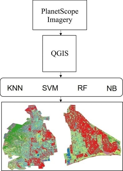
2.4. Methodology Flowchart

An overview of the methodology used in this study is presented in Figure 2. First, we acquired aerial satellite data in three phases: data collection, pre-processing, results and analysis. The LULC classification maps were determined using the RF, SVM, NB and KNN algorithms to assess their accuracies in dense urban areas. Several satellite images covered each study area, and it was necessary to split all imagery into four bands (R, G, B and NIR). Same bands from different images were merged without resampling as they all had the exact resolution, thus creating four-band composition imagery built from merged bands as separate layers. Supervised classification requires composite satellite imagery and trained samples. Therefore, based on the study’s objective, four classes were created: (1) vegetation, (2) water bodies, (3) built-up and (4) trees. Built-up class consisted of all urban features that could not be categorised in any of the other classes, such as buildings, roads, pavement and soil. Due to the number of four classes created, a multi-class classification resulted, which results when more than two class labels exist within the classification. A polygon shapefile was created, and different classes were randomly digitised throughout the study area from the satellite imagery. A unique ID was allocated to all digitised features; for instance, all water bodies were assigned ID 2, while trees were assigned ID 4. Southern Suburbs had 213 training samples, while Cape Flats had 340 samples. Large classification areas need more training samples compared to small areas.

2.5. Validation

To validate the classification results, we followed best practices for accuracy assessments by Olofsson et al. [50] based on randomly distributed points throughout the study area, which were derived from high-resolution aerial photographs obtained from the CoCT. Classification results were superimposed over aerial photographs, and visual inspections were conducted over the data to assess the accuracy. During image classification, 80% of the training samples were used to train the classifiers, while 20% were used for validating the results. Cape Flats had 340 training samples. Therefore, 68 (20%) was used for validation, while 272 (80%) was used to train the classifier. For the Southern Suburbs, 43 (20%) were used to validate results, while 170 (80%) were used to train the classifier. The four land use classes were digitised as polygons from aerial imagery and were therefore part of training samples. These training samples were distributed throughout the study area. A systematic comparison approach is also used to validate the quality of thematic classification maps against maps derived from remote sensing [51]. In this case, all four produced classification maps were visually compared with each other for cross-checking results. We then created a confusion matrix and calculated the overall accuracy (OA), including the Kappa coefficient (k), for determining whether one error matrix was significantly different from another [52], calculated from Equations (1) and (2):

$$OA=\frac{Number of correctly classified pixels }{Total number of pixels}$$

(1)

$$k=\frac{N{\sum }_{i=1}^r{x}_{ii}-{\sum }_{i=1}^r\left(x_{i+1}\times x_{+i}\right)}{N^2-{\sum }_{i=1}^r(x_{i+}\times x_{+i})}$$

(2)

where r = the number of rows and columns in the error matrix; x_ii = the number of observations in row i and column i; x_i+ = the marginal sum of row i; x_+i = the marginal sum of column i; and N = the total number of observations.

3. Results

This study focused on classifying the main LULC classes using RF, SVM, KNN and NB classifiers based on high-resolution PlanetScope data for 2016 and 2021. We then performed a change detection and characterised the LULC that transpired during this period to understand the human footprint there. We first present the performance of the classifiers and then report the changes in both the Southern Suburbs and the Cape Flats.

3.1. Urban Land Use and Land Cover Classification

The four LULC classes of vegetation, water bodies, built-up and trees and the comparison of four classification strategies for 2016 and 2021, are shown in Figure 3 for the Southern Suburbs. We found a relatively similar spatial configuration in LULC categories in Southern Suburbs. The central interior to the western section was dominated by the vegetative cover, sprinkled with trees toward the edge, and the eastern section was concentrated with built-up land. The water bodies showed a patchy distribution, mainly in the northwest and southeast sections of the area. The statistical accuracies for all classifiers in the Southern Suburbs are summarised in

Table 2. Urban land use and land cover classification accuracies for the Southern Suburbs in 2016 and 2021.

Class	RF		SVM		NB		KNN
	2016	2021	2016	2021	2016	2021	2016	2021
Built-up	0.99	0.82	0.98	0.79	0.98	0.82	0.99	0.90
Trees	0.98	0.96	0.98	0.96	0.97	0.94	0.99	0.95
Vegetation	0.88	0.93	0.92	0.93	0.88	0.96	0.94	0.97
Waterbodies	0.99	0.99	0.99	0.98	0.99	0.94	0.99	0.98
Overall accuracy (%)	96.62	94.8	97.44	92.28	96.37	93.71	98.31	96.54
Kappa Coefficient	0.94	0.92	0.92	0.88	0.94	0.91	0.97	0.95

RF = Random forests; SVM = Support vector machines; NB = Native Bayes; KNN = K-Nearest Neighbour.

. Generally, the classification results for 2016 showed higher accuracies than for 2021. Classification accuracies for LULC ranged from 92.28% to 98.31%, with KNN consistently performing the best in both study periods (Table 2). The KNN achieved an overall accuracy of 98.31% (Kappa 0.97) and 96.54% (Kappa of 0.95) for 2016 and 2021, respectively. The RF attained 96.62% (Kappa 0.94) and 94.8% (Kappa 0.92) in the corresponding years. Similarly, SVM achieved an accuracy of 97.44% (Kappa 0.92) and 92.28% (Kappa 0.88), respectively. The NB also had an overall accuracy of 96.37% (Kappa 0.94) and 93.71% (Kappa 0.91), respectively. Within LULC categories, higher accuracies were achieved for water bodies (Table 2).

The results of the classification in the Cape Flats are presented in Figure 4. It is obvious that towards the east and centre, there has been an increase in built-up land from 2016 to 2021. Towards the western section, the number of trees decreased notably in 2021 compared to 2016, with an increase in vegetation and urban infrasturcture dominating. The southeast waterbodies remained relatively stable in both 2016 and 2021. The statistical accuracies for all classifiers are summarised in

Table 3. Urban land use and land cover classification accuracies for the Cape Flats in 2016 and 2021.

Class	RF		SVM		NB		KNN
	2016	2021	2016	2021	2016	2021	2016	2021
Built-up	0.91	0.98	0.93	0.99	0.89	0.98	0.98	0.99
Trees	0.98	0.99	0.96	0.96	0.94	0.91	0.97	0.96
Vegetation	0.89	0.88	0.91	0.92	0.95	0.92	0.97	0.94
Waterbodies	0.99	0.99	0.99	0.99	0.99	0.99	0.99	0.99
Overall accuracy (%)	94.8	96.77	95.85	98.04	95.37	97.54	98.56	98.43
Kappa Coefficient	0.91	0.94	0.93	0.92	0.92	0.95	0.98	0.97

RF = Random forests; SVM = Support vector machines; NB = Native Bayes; KNN = K-Nearest Neighbour.

. Again, KNN outperformed the other classifiers for 2016 and 2021 with overall accuracies of 98.56% (Kappa 0.98) and 98.43% (Kappa 0.97), respectively. For the same period, the SVM had an overall classification accuracy of 95.85% (Kappa 0.930) and 98.04% (Kappa 0.92), respectively. The NB achieved an overall accuracy of 95.37% (Kappa 0.92) and 97.54% (Kappa 0.95). Lastly, RF achieved 94.8% (Kappa 0.91) and 96.77% (Kappa 0.94) for 2016 and 2021, respectively.

3.2. Urban Land Use and Land Cover Change Analysis

3.2.1. Southern Suburbs

The spatial distribution of LULC changes and conversion between 2016 and 2021 in the Southern Suburbs is shown in Figure 5 and Figure 6, respectively. As expected, the built-up class showed more stability, and the transformation of other LULC classes, particularly vegetation (mostly in the interior) and trees (in the eastern section), was evident.

3.2.2. Cape Flats

The spatial distribution of LULC changes and conversion between 2016 and 2021 in the Cape Flats is shown in Figure 7 and Figure 8, respectively. Due to the nature of Cape Flats as a developing suburb, some vegetation and trees were expected to be destroyed during the construction of homes and other infrastructure. In this case, trees were replaced by built-up areas towards the southeastern section. On the southern border, most of the trees have turned into vegetation. In addition, the waters seem to be stable, and no major changes are observed.

Regarding land use in the Cape Flats in 2021, Figure 9a represents reserved land occupied by informal households. Figure 9b illustrates additional households constructed from the original town plan design, demarcated in the red polygon. During construction, trees are destroyed and not replaced in other areas. Vacant land reserved for other town planning purposes is invaded and informal housing structures are constructed. During this practice, vegetation and trees are destroyed. Informal households’ construction has occupied much land and it has become difficult to plant trees.

4. Discussion

Our results showed that machine learning algorithms produced approximately equivalent accuracy, with the KNN classifier showing the best performance in 2016 and 2021. Similarly, Balcik et al. [46] used Sentinel-2 and SPOT-7 images to classify greenhouses in Anamur, Turkey, with KNN, RF and SVM classifiers. The authors found that KNN achieved the highest overall accuracy of 88.38% (0.83 Kappa) on Sentinel-2 images. Bardadi et al. [44] also studied LULC changes over Tlemcen, Algeria, after forest fire damage and found a high performance of the KNN classifier. Noi and Kappas [45] compared KNN, RF and SVM for LULC classification using Sentinel-2 imagery over the Red River Delta, Viet, and their results showed a high overall accuracy ranging from 90% to 95%, with SVM at 95.29%, RF at 94.59% and KNN at 94.10%. Though SVM produced the highest overall accuracy, results from KNN and RF were still considered within high overall accuracy and were therefore usable for further analysis. Balcik et al. [46] used Sentinel-2 and SPOT-7 satellite products to classify greenhouses in Anamur, Turkey, with KNN, RF and SVM classifiers, where the KNN achieved the highest overall accuracy of 88.38% and 0.83 Kappa on Sentinel-2 images, while on SPOT-7, both KNN and RF achieved an overall accuracy of 91.43% and 0.88 Kappa. Most notably, classification results in this study have ignorable variances, and this finding is consistent with [53,54]

Trees are the most critical elements in urban areas due to their ecosystem services, role in urban environmental management, and effect on the urban heat island [55]. The KNN achieved the highest overall accuracy in the Southern Suburbs for 2016, followed by SVM, RF and NB. In 2021, the highest overall accuracy in the Southern Suburbs was the KNN, followed by RF, NB, and SVM. The Cape Flats’ 2016 image classification showed that KNN achieved the highest overall accuracy, followed by, SVM, NB and RF. In contrast, the 2021 image classification showed KNN with the highest overall accuracy followed by, SVM, NB and RF. Notably, all classifiers’ overall accuracy was above 90%, which informed the reliability of LULC maps produced in this study. Though KNN achieved the highest overall accuracy, results from other classifiers are still acceptable, and their LULC maps can be used for planning purposes.

The authors discovered that some areas were misclassified while visually inspecting and superimposing the 2021 LULC maps over 2021 aerial images provided by CoCT. Specifically, trees were classified as vegetation or vice versa, and this happened in areas where the vegetation was green. Therefore, in such instances, LiDAR data and the height threshold can be applied to eliminate this error. However, LiDAR data are not always available, as they are expensive to collect over large areas. The LULC change analyses were performed over five years in both suburbs, and it was possible to determine the changes that occurred. The LULC occurred differently between the affluent Southern Suburbs and the less-affluent Cape Flats. In Cape Flats, there was an increase of 0.04% in tree canopy in areas previously classified as built-up areas. However, 2.7% of trees were lost to built-up areas over five years, as in the case of middle-class suburbs undergoing development programmes. Thus, most trees were lost in Cape Flats over a period of 5 years. In contrast, the more developed Southern Suburbs showed an increase of 0.01% in built-up areas to tree canopy over a period of 5 years; this is attributed to the fact that less development is expected in planned suburbs. There was, however, a further loss of trees to vegetation amounting to 7.5%.

Interpreting Figure 6 for land use and land cover (LULC) conversion between 2016 and 2021 in the Southern Suburbs over a 5-year period, the following changes are noted: 23.9% of vegetation remains unchanged, 0.1% water body to vegetation, 0.8% built-up to vegetation, 0.2% water body unchanged, 0.6% trees to water body, 21.5% vegetation to built-up, 0.2% water body to built-up, 22.3% built-up unchanged, 2.6% trees to built-up and vegetation to trees and 16.6% trees unchanged.

In contrast Figure 8, aerial urban land use and land cover (LULC) conversion between 2016 and 2021 over the Cape Flats is as follows: 17.3% vegetation unchanged, 0.3% water body to vegetation, 4% built-up to vegetation, 9.6% trees to vegetation, 0.3% vegetation to water body, 1.7% water body unchanged, 0.2% built-up to water body, 14.9% vegetation to built-up, 0.3% water body to built-up, 44.2% built-up unchanged, 2.7% trees to built-up, 0.8% Vegetation to trees, 0.5% water body to trees and, lastly, 3% trees unchanged.

In LULC classification studies, it is advisable to have soil as a separate class instead of merging it with general built-up items. Soil class can also inform those responsible for planting trees about the available area that can be utilised. However, this study’s objective was to quantify tree canopy using remote sensing techniques and evaluate machine learning algorithms’ accuracy. Several researchers have evaluated the spatial patterns and dynamics of LULC to assess its use in preserving ecological stability. For example, Abdi [56] studied the LULC of boreal landscapes in south-central Sweden using Sentinel-2 image by applying SVM, FR, extreme gradient boosting (Xgboost) and deep learning machine learning algorithms. Tavares et al. [57] mapped LULC using Sentinel-1 and Sentinel-2 in Belém, Eastern Brazil Amazon, applying an RF classifier. The KNN classifier was used by Meng et al. [58] to map forest inventory using remote sensing data in Marion County, Georgia. These studies show that LULC gained popularity in remote sensing to analyse spatial patterns. Easily accessible satellite images and improvements in computer processing abilities motivate the application of remote sensing in urban studies, specifically spatial patterns.

5. Conclusions and Outlook

The objective of this study was to compare four machine learning classifier techniques based on PlanetScope imagery, followed by evaluating the accuracy metrics. Our results showed the capability of machine learning algorithms based on PlanetScope imagery for classifying LULC in heterogeneous urban landscapes with high thematic fidelity. The KNN classifier outperformed all classifiers for both study years, which constituted four experiments, and waterbodies consistently had high overall accuracy in all cases. However, all the results produced by other classifiers had an overall accuracy above 90%, so they can still be used for different types of analysis and decision making. It is noteworthy that there have been few studies in South Africa using a similar methodology, leaving room for improvement in future research. The middle-class Cape Flats are characterised by potential for future development projects that could have a definitive impact on LULC in this area. The affluent Southern Suburbs showed an increase in tree canopy over the study period. In particular, there are limited future construction projects in developed suburbs as opposed to developing suburbs, and therefore, fewer trees are lost. However, in this study, KNN showed high performance on the PlanetScope image in mapping urban LULC. Therefore, our findings are not inconsistent with studies that have found high performance of KNN.

While our analyses yielded LULC maps with great thematic fidelity, a few uncertainties remain. First, due to the healthy composition of the vegetation areas, a negligible number of trees were classified as vegetation. This is caused by a similar reflectance from both tree canopy and vegetation. However, the authors ruled out the possibility of image misclassification by using 2016 and 2021 satellite images taken in the same season, as vegetation and trees are subject to weather changes. The literature shows that LULC studies are typically conducted over 10 years. However, the authors decided on five years because of PlanetScope data available for both Cape Flats and Southern Suburbs included 2016 to 2021. Therefore, it was not possible to map LULC changes over 10 years.

Future urban studies can deploy the methodology outlined in this study to track changes within cities and, more importantly, tree canopy cover in countries committed to adopting a green city ideology. This application can also be extended to mining areas to map rehabilitation dynamics. The high-resolution PlanetScope imagery can help provide stakeholders with accurate information that can be used during land management decision-making.

References

1. Haines-Young, R. Land use and biodiversity relationships. Land Use Policy 2009, 26, S178–S186. [Google Scholar] [CrossRef]
2. Bolund, P.; Hunhammar, S. Ecosystem services in urban areas. Ecol. Econ. 1999, 29, 293–301. [Google Scholar] [CrossRef]
3. Hu, T.; Yang, J.; Li, X.; Gong, P. Mapping urban land use by using Landsat images and open social data. Remote Sens. 2016, 8, 151. [Google Scholar] [CrossRef]
4. McConnachie, M.M.; Shackleton, C.M. Public green space inequality in small towns in South Africa. Habitat. Int. 2010, 34, 244–248. [Google Scholar] [CrossRef] [Green Version]
5. Nesbitt, L.; Meitner, M.J. Exploring relationships between socioeconomic background and urban greenery in Portland, OR. Forests 2016, 7, 162. [Google Scholar] [CrossRef] [Green Version]
6. Ablo, A.D.; Asem, F.E.; Yiran, G.A.; Owusu, G. Urban sprawl, land use change and the changing rural agrarian livelihood in peri-urban Accra, Ghana. Rural-Urban Link. Sustain. Dev. Case Stud. Afr. 2020, 16, 77–100. [Google Scholar]
7. Soni, P.K.; Rajpal, N.; Mehta, R.; Mishra, V.K. Urban Land cover and land use classification using multispectral Sentinel-2 imagery. Multimed. Tools Appl. 2021, 1–15. [Google Scholar] [CrossRef]
8. Klein, D.; Esch, T.; Himmler, V.; Thiel, M.; Dech, S. Assessment of urban extent and imperviousness of Cape Town using TerraSAR-X and Landsat images. In Proceedings of the 2009 IEEE International Geoscience and Remote Sensing Symposium, Cape Town, South Africa, 12–17 July 2009; Volume 3, p. III-1051. [Google Scholar]
9. Kavitha, A.V.; Srikrishna, A.; Satyanarayana, C. A review on detection of land use and land cover from an optical remote sensing image. IOP Conf. Ser. Mater. Sci. Eng. 2021, 1074, 012002. [Google Scholar] [CrossRef]
10. Yang, X.; Lo, C.P. Modelling urban growth and landscape changes in the Atlanta metropolitan area. Int. J. Geogr. Inf. Sci. 2003, 17, 463–488. [Google Scholar] [CrossRef]
11. Haack, B.N.; Rafter, A. Urban growth analysis and modeling in the Kathmandu valley, Nepal. Habitat. Int. 2006, 30, 1056–1065. [Google Scholar] [CrossRef]
12. Wu, C.; Deng, C.; Jia, X. Spatially constrained multiple endmember spectral mixture analysis for quantifying subpixel urban impervious surfaces. IEEE J. Sel. Top. Appl. Earth Obs. Remote Sens. 2014, 7, 1976–1984. [Google Scholar] [CrossRef]
13. Cai, C.; Li, P.; Jin, H. Extraction of urban impervious surface using two-season Worldview-2 images: A comparison. Photogramm. Eng. Remote Sens. 2016, 82, 335–349. [Google Scholar] [CrossRef]
14. Zhang, T.; Huang, X. Monitoring of urban impervious surfaces using time series of high-resolution remote sensing images in rapidly urbanized areas: A case study of Shenzhen. IEEE J. Sel. Top. Appl. Earth Obs. Remote Sens. 2018, 11, 2692–2708. [Google Scholar] [CrossRef]
15. Barr, S.L.; Barnsley, M.J.; Steel, A. On the separability of urban land-use categories in fine spatial scale land-cover data using structural pattern recognition. Environ. Plan. B Plan. Des. 2004, 31, 397–418. [Google Scholar] [CrossRef]
16. Woodcock, C.E.; Strahler, A.H. The factor of scale in remote sensing. Remote Sens. Environ. 1987, 21, 311–332. [Google Scholar] [CrossRef]
17. Li, M.; Stein, A. Mapping land use from high resolution satellite images by exploiting the spatial arrangement of land cover objects. Remote Sens. 2020, 12, 4158. [Google Scholar] [CrossRef]
18. Lu, D.; Weng, Q. Use of impervious surface in urban land-use classification. Remote Sens. Environ. 2006, 102, 146–160. [Google Scholar] [CrossRef]
19. Shaban, M.A.; Dikshit, O. Improvement of classification in urban areas by the use of textural features: The case study of Lucknow city, Uttar Pradesh. Int. J. Remote Sens. 2001, 22, 565–593. [Google Scholar] [CrossRef]
20. Zhang, S.; Miao, Y.; Li, X.; He, H.; Sang, Y.; Du, X. Determining next best view based on occlusion information in a single depth image of visual object. Int. J. Adv. Robot. Syst. 2016, 14, 1729881416685672. [Google Scholar] [CrossRef] [Green Version]
21. Blaschke, T. Object based image analysis for remote sensing. ISPRS J. Photogramm. Remote Sens. 2010, 65, 2–16. [Google Scholar] [CrossRef] [Green Version]
22. Duro, D.C.; Franklin, S.E.; Dubé, M.G. A comparison of pixel-based and object-based image analysis with selected machine learning algorithms for the classification of agricultural landscapes using SPOT-5 HRG imagery. Remote Sens. Environ. 2012, 118, 259–272. [Google Scholar] [CrossRef]
23. Shi, Y.; Qi, Z.; Liu, X.; Niu, N.; Zhang, H. Urban land use and land cover classification using multisource remote sensing images and social media data. Remote Sens. 2019, 11, 2719. [Google Scholar] [CrossRef] [Green Version]
24. Ha, T.V.; Tuohy, M.; Irwin, M.; Tuan, P.V. Monitoring and mapping rural urbanization and land use changes using landsat data in the northeast subtropical region of Vietnam. Egypt J. Remote Sens. Space Sci. 2020, 23, 11–19. [Google Scholar] [CrossRef]
25. Kranjčić, N.; Medak, D.; Župan, R.; Rezo, M. Machine learning methods for classification of the green infrastructure in city areas. ISPRS Int. J. Geo-Inf. 2019, 8, 463. [Google Scholar] [CrossRef] [Green Version]
26. Van Weele, G.; Maree, G. State of Environment Outlook Report for the Western Cape Province: Introductory Matter; Western Cape Government Environmental Affairs Development Planning: Cape Town, South Africa, 2013. [Google Scholar]
27. Food and Agriculture Organization (FAO) of the United Nations. FAOSTAT; Food and Agriculture Organization of the United Nations: Rome, Italy, 2020. [Google Scholar]
28. ArbNet. Available online: https://www.capetownetc.com/news/cape-town-completes-countrys-first-city-tree-mapping/ (accessed on 10 December 2021).
29. Planet_Imagery Product Specification [WWW Document]. Available online: https://assets.planet.com/docs/Planet_Combined_Imagery_Product_Specs_letter_screen.pdf (accessed on 19 March 2022).
30. Breiman, L. Random Forests. Mach. Learn. 2001, 45, 5–32. [Google Scholar] [CrossRef] [Green Version]
31. Belgiu, M.; Drăguţ, L. Random forest in remote sensing: A review of applications and future directions. ISPRS J. Photogramm. Remote Sens. 2016, 114, 24–31. [Google Scholar] [CrossRef]
32. Richetti, J.; Boote, K.J.; Hoogenboom, G.; Judge, J.; Johann, J.A.; Uribe-Opazo, M.A. Remotely sensed vegetation index and lai for parameter determination of the CSM-CROPGRO-soybean model when in situ data are not available. Int. J. Appl. Earth Obs. Geoinf. 2019, 79, 110–115. [Google Scholar] [CrossRef]
33. Woznicki, S.A.; Baynes, J.; Panlasigui, S.; Mehaffey, M.; Neale, A. Development of a spatially complete floodplain map of the conterminous United States using random forest. Sci. Total Environ. 2019, 647, 942–953. [Google Scholar] [CrossRef]
34. Biau, G.; Scornet, E. A random forest guided tour. Test 2016, 25, 197–227. [Google Scholar] [CrossRef] [Green Version]
35. Rodriguez-Galiano, V.F.; Ghimire, B.; Rogan, J.; Chica-Olmo, M.; Rigol-Sanchez, J.P. An assessment of the effectiveness of a random forest classifier for land-cover classification. ISPRS J. Photogramm. Remote Sens. 2012, 67, 93–104. [Google Scholar] [CrossRef]
36. Sexton, T.; Brundage, M.P.; Hoffman, M.; Morris, K.C. Hybrid datafication of maintenance logs from AI-assisted human tags. In Proceedings of the 2017 IEEE International Conference on Big Data, Boston, MA, USA, 11–14 December 2017; pp. 1769–1777. [Google Scholar]
37. Susto, G.A.; McLoone, S.; Pagano, D.; Schirru, A.; Pampuri, S.; Beghi, A. Prediction of integral type failures in semiconductor manufacturing through classification methods. In Proceedings of the 2013 IEEE 18th Conference on Emerging Technologies & Factory Automation (ETFA), Cagliari, Italy, 10–13 September 2013; pp. 1–4. [Google Scholar]
38. Mustafa, A.; Rienow, A.; Saadi, I.; Cools, M.; Teller, J. Comparing support vector machines with logistic regression for calibrating cellular automata land use change models. Eur. J. Remote Sens. 2018, 51, 391–401. [Google Scholar] [CrossRef]
39. Taskin Kaya, G.; Musaoglu, N.; Ersoy, O.K. Damage assessment of 2010 Haiti earthquake with post-earthquake satellite image by support vector selection and adaptation. Photogramm. Eng. Remote Sens. 2011, 77, 1025–1035. [Google Scholar] [CrossRef]
40. Zhou, X.; Li, L.; Chen, L.; Liu, Y.; Cui, Y.; Zhang, Y.; Zhang, T. Discriminating urban forest types from Sentinel-2A image data through linear spectral mixture analysis: A case study of Xuzhou, east China. Forests 2019, 10, 478. [Google Scholar] [CrossRef] [Green Version]
41. Dabija, A.; Kluczek, M.; Zagajewski, B.; Raczko, E.; Kycko, M.; Al-Sulttani, A.H.; Tardà, A.; Pineda, L.; Corbera, J. Comparison of support vector machines and random forests for CORINE land cover mapping. Remote Sens. 2021, 13, 777. [Google Scholar] [CrossRef]
42. Guo, G.; Wang, H.; Bell, D.; Bi, Y.; Greer, K. KNN model-based approach in classification. In Proceedings of the OTM Confederated International Conferences “On the Move to Meaningful Internet Systems”, Sicily, Italy, 3–7 November 2003; pp. 986–996. [Google Scholar]
43. Atkeson, C.G.; Moore, A.W.; Schaal, S. Locally weighted learning. Artif. Intell. Rev. 1997, 11, 11–73. [Google Scholar] [CrossRef]
44. Bardadi, A.; Souidi, Z.; Cohen, M.; Amara, M. Land use/land cover changes in the Tlemcen region (Algeria) and classification of fragile areas. Sustainability 2021, 13, 7761. [Google Scholar] [CrossRef]
45. Thanh Noi, P.; Kappas, M. Comparison of random forest, k-nearest neighbor, and support vector machine classifiers for land cover classification using Sentinel-2 imagery. Sensors 2017, 18, 18. [Google Scholar] [CrossRef] [Green Version]
46. Balcik, F.B.; Senel, G.; Goksel, C. Object-based classification of greenhouses using Sentinel-2 MSI and SPOT-7 images: A case study from Anamur (Mersin), Turkey. IEEE J. Sel. Top. Appl. Earth Obs. Remote Sens. 2020, 13, 2769–2777. [Google Scholar] [CrossRef]
47. Zhang, H. The optimality of naive bayes. Aa 2004, 1, 3. [Google Scholar]
48. Camargo, F.F.; Sano, E.E.; Almeida, C.M.; Mura, J.C.; Almeida, T. A Comparative assessment of machine-learning techniques for land use and land cover classification of the Brazilian tropical savanna using ALOS-2/PALSAR-2 Polarimetric images. Remote Sens. 2019, 11, 1600. [Google Scholar] [CrossRef] [Green Version]
49. Wei, C.; Huang, J.; Mansaray, L.R.; Li, Z.; Liu, W.; Han, J. Estimation and mapping of winter oilseed rape LAI from high spatial resolution satellite data based on a hybrid method. Remote Sens. 2017, 9, 488. [Google Scholar] [CrossRef] [Green Version]
50. Olofsson, P.; Foody, G.M.; Herold, M.; Stehman, S.V.; Woodcock, C.E.; Wulder, M.A. Good practices for estimating area and assessing accuracy of land change. Remote Sens. Environ. 2014, 148, 42–57. [Google Scholar] [CrossRef]
51. Vicente-Serrano, S.M.; Gouveia, C.; Camarero, J.J.; Beguería, S.; Trigo, R.; López-Moreno, J.I.; Azorín-Molina, C.; Pasho, E.; Lorenzo-Lacruz, J.; Revuelto, J. Response of vegetation to drought time-scales across global land biomes. Proc. Natl. Acad. Sci. USA 2013, 110, 52–57. [Google Scholar] [CrossRef] [PubMed] [Green Version]
52. Congalton, R.G.; Green, K. Assessing the Accuracy of Remotely Sensed Data: Principles and Practices; Lewis Publishers: Boca Rotan, FL, USA, 1999. [Google Scholar]
53. Erbek, F.S.; Özkan, C.; Taberner, M. Comparison of maximum likelihood classification method with supervised artificial neural network algorithms for land use activities. Int. J. Remote Sens. 2004, 25, 1733–1748. [Google Scholar] [CrossRef]
54. Adam, E.; Mutanga, O.; Odindi, J.; Abdel-Rahman, E.M. Land-use/cover classification in a heterogeneous coastal landscape using Rapid Eye imagery: Evaluating the performance of random forest and support vector machines classifiers. Int. J. Remote Sens. 2014, 35, 3440–3458. [Google Scholar] [CrossRef]
55. Wilkes, P.; Disney, M.; Vicari, M.B.; Calders, K.; Burt, A. Estimating urban above ground biomass with multi-scale LiDAR. Carbon Balance Manag. 2018, 13, 10. [Google Scholar] [CrossRef]
56. Abdi, A.M. Land Cover and land use classification performance of machine learning algorithms in a boreal landscape using Sentinel-2 data. GISci. Remote Sens. 2020, 57, 1–20. [Google Scholar] [CrossRef] [Green Version]
57. Tavares, P.A.; Beltrão, N.E.S.; Guimarães, U.S.; Teodoro, A.C. Integration of Sentinel-1 and Sentinel-2 for classification and lulc mapping in the urban area of Belém, Eastern Brazilian Amazon. Sensors 2019, 19, 1140. [Google Scholar] [CrossRef] [Green Version]
58. Meng, Q.; Cieszewski, C.J.; Madden, M.; Borders, B.E. K nearest neighbor method for forest inventory using remote sensing data. GISci. Remote Sens. 2007, 44, 149–165. [Google Scholar] [CrossRef]
Figure 1. Location of the study areas in the City of Cape Town, South Africa.
Sustainability 14 09139 g001
Figure 2. Methodology flowchart.
Sustainability 14 09139 g002
Figure 3. True colour Plant Scope Imagery, Random Forests (RF), Support Vector Machine (SVM), K-nearest neighbour (KNN) and Naïve Bayes (NB) classifiers for 2016 (top panels); True colour Plant Scope Imagery, RF, SVM, KNN and NB classifiers for 2021 (bottom panels) of Southern Suburbs.
Sustainability 14 09139 g003
Figure 4. True colour Plant Scope Imagery, Random Forests (RF), Support Vector Machine (SVM), K-nearest neighbour (KNN) and Naïve Bayes (NB) classifiers for 2016 (top panels); True colour Plant Scope Imagery, RF, SVM, KNN and NB classifiers for 2021 (bottom panels) of Cape Flats.
Sustainability 14 09139 g004
Figure 5. Southern Suburbs spatial representation of urban land use and land cover (LULC) conversion from 2016 to 2021.
Sustainability 14 09139 g005
Figure 6. Areal urban land use and land cover (LULC) conversion between 2016 and 2021 over the Southern Suburbs.
Sustainability 14 09139 g006
Figure 7. Cape Flats spatial representation of urban land use and land cover (LULC) conversion from 2016 to 2021.
Sustainability 14 09139 g007
Figure 8. Areal urban land use and land cover (LULC) conversion between 2016 and 2021 over the Cape Flats.
Sustainability 14 09139 g008
Figure 9. Land use in the Cape Flats in 2021: (a) represents reserved land occupied by informal households, and (b) represents additional households constructed from the original town plan design, demarcated in red polygon.
Sustainability 14 09139 g009