Construction of an Ecological Network Based on an Integrated Approach and Circuit Theory: A Case Study of Panzhou in Guizhou Province

Abstract

Protecting ecological security has become the backbone of social and economic development since declines in ecological quality due to an increase in human dominance over the natural environment. The establishment of ecological networks is an effective, comprehensive spatial regulation means to ensure regional ecological security. Panzhou city, as a case study, is a typical karst county and has been confronted with the pressure of ecological degradation in recent decades. In this study, an integrated approach combining ecological quality (EQ), ecosystem function importance (EFI), and morphological spatial pattern analysis (MSPA) was developed to determine the ecological sources. Ecological corridors, ecological pinch areas, and ecological barriers were extracted using circuit theory to identify the restored and conserved priority areas of ecological security patterns. The results showed that (1) the remote sensing ecological index (RSEI) and EFI exhibited typical geographical distributions, with the highest values concentrated in the northern and southern parts of the study area and the lowest values scattered in the middle part; (2) 26 patches with forestland, grassland, and waterbodies as the main land cover types were selected as the ecological sources; (3) 63 ecological corridors, composed of 45 key ecological corridors and 18 inactive ecological corridors, were extracted, accounting for 203.12 km and 163.31 km, respectively; (4) 82.76 km² of pinch areas and 320.29 km² of barriers were identified, both of which were distributed on key ecological corridors and played different roles in ecological security; and (5) 4 types of ecological security zones were established according to ecological sources, corridors, pinch areas, and barriers. This integrated approach provides a scientific method for the identification and implementation of ecological networks that can contribute to protecting regional ecological security. Our findings can serve as applicable and reasonable guidance to land administrators and policy-makers for adopting suitable territorial spatial planning, urban planning, green cities, etc.

1. Introduction

Regional increasing urbanization and industrialization due to the increase in the human population have caused serious, diverse, and negative impacts on ecosystems [1,2]. Ecological degradation, such as loss of biodiversity and habitat fragmentation, is increasing [3]. Thus, the sustainable development of human society and ecological security are experiencing severe challenges [4,5]. Since the 18th CPC National Congress, the construction of ecological civilization has become an important strategic goal in regional development. The Fifth Plenary Session of the 19th CPC Central Committee put forward strategic goals to increase ecological progress, strengthen ecological security barriers, and significantly improve the urban and rural living environment [6]. Restoring the broken ecological space and promoting the healthy development of the ecosystem has become a major task of ecological civilization and territorial spatial planning in China [7]. In this context, constructing a profitable ecological security pattern is seen as the most profitable strategy for ecological protection [8].

In recent years, studies on ecological security patterns that have been conducted in different countries around the world indicated that the establishment of ecological networks is an effective means of comprehensive spatial regulation to ensure regional ecological security [9,10,11,12,13]. An ecological network can be described as a mutualistic web to functionally connect habitat patches, facilitate the dispersal of species, and therefore support the survival of numerous species typical to natural and semi-natural habitats [14]. Since the 1980s, establishing an appropriate designation and identification method has been the key to an eco-logical network. A basic research paradigm for the ecological network was developed, that is, determining ecological sources–constructing ecologically resistant surfaces–extracting ecological corridors [15,16,17]. An increasing number of researchers have focused on the application and improvement of this paradigm [18,19,20].

The ecological sources are the basic elements in an ecological network, which can provide decisive functions in the ecological network, for instance, a stable habitat for animals, high quality ecological patches for human beings. Currently, ecological sources can be identified through two methods: on the one hand, based on empirical judgment from the experiences and expertise of researchers, natural landscape elements—such as nature reserves, large forestry, scenic spots, and wetland parks—were directly selected as ecological sources after qualitative analysis [21,22], but this method was subjective and ignored the effective measurement of the ecological state of the patches after being impacted by human activities. On the other hand, a series of evaluation frameworks of ecological importance have been used to identify the ecological sources, where ecological indicators [23], ecological functions [24], or the ecological suitability index [25] were widely adopted in practice. More importantly, these frameworks made it possible to find an effective solution to protect a targeted zone, and it is more reasonable to rank patches based on their degree of ecological importance than on the land attributes [26]. However, due to the lack of evaluation principles of ecological importance, scholars often used different evaluation indicators to evaluate ecological importance according to regional characteristics or protection objectives, such as species conservation [27], ecological functions for the terrestrial ecosystem and the aquatic ecosystem [28], habitat importance [29], or blue infrastructure (BI) [30]. In this study, an integrated method was proposed to comprehensively evaluate ecological importance in an effort to improve regional ecosystem structure, ecosystem function, and ecological quality. Based on the result of the assessment, patches with superior importance in ecosystem structure, ecosystem function, and ecological quality were demarcated as ecological sources.

The resistance surface refers to the cost of landscape media to overcome interpatch flow resistances and can reflect the inherent influence of landscape heterogeneity on the ecological flow [31,32]. The resistance surface is essential for an ecological network and even a regional ecological security model. There are many different methods in terms of defining and establishing the resistance surface [2,28,33,34]. Because of the different geographical locations, methodologies may differ. The resistance surface was firstly analyzed and determined based on land-use types [29], and then the relevant indicators were involved, some of which were related to human activities, such as night-time light intensity [28], or urban expansion, such as the distance from residential areas [32]. At the same time, some studies revealed that the ecological resistance depended on the ecological quality, and the units with higher quality had smaller resistance. It was gradually realized that the ecosystems had evolved into a highly artificial natural–socio compound ecosystem due to the serious disturbance from rapid urbanization and industrialization. Hence, adjusting a reasonable ecological resistance surface based on these human disturbances has become an important recent trend. In this study, four classes of factors were used to estimate the resistance surface, namely, the topography of the study area, vegetation status, human activities, and quantitative indexes reflecting the typical fragile ecological environment of the study area.

The ecological corridor is commonly defined as a linear or ribbon ecological landscape, which has the functions of natural habitat and serves a smooth channel for the flow of materials, energy, and organism between core patches of ecological sources [17,35,36]. At present, the minimum cumulative resistance (MCR) model and circuit theory are mainly applied to identify corridors. The MCR can consider the internal relationship between land cover units and identify the optimal direction and route of biological flows. Since it was introduced in 1996 [37,38], the MCR has been widely used in the study of ecological security patterns [39]. However, the MCR cannot clarify the spatial range and key nodes of an ecological corridor that could hinder or weaken ecological flow [28]. Circuit theory simulates the diffusion process of species in an ecosystem by applying the random walk characteristics of electrons in a circuit [40,41]. The essential advantage of circuit theory is that it can identify the key positions according to the current intensity and determine the width thresholds of ecological corridors according to the frequency distribution of the current values. Therefore, the circuit theory has gained increasing attention and was used in this study.

Located in southwestern China, Panzhou city is a typical karst county in Guizhou Province. Like other county-level regions in China, it has faced the problem of ecological degradation originating from rapid development over the last few decades. Furthermore, as one of the most prominent karst landform areas, it also has confronted notable pressure to balance its ecological protection and economic growth. However, its vulnerable ecosystem provides a distinctive landscape and necessary habitat for rare plants and animals, which can contribute to the ecotourism industry, one of the province’s predominant economic services. Despite its profound ecological advantages or disadvantages, research work on ecological security patterns and the construction of an ecological network in karst areas has rarely been explored in the literature. Therefore, in this study, ecological quality (EQ), ecosystem function importance (EFI), and morphological spatial pattern analysis (MSPA) were assessed, and the ecological sources were identified according to the superior importance of the EQ, EFI, and MSPA, respectively. Using topography, vegetation status, human activities, and quantitative indexes, the resistance surface was established, and the circuit theory was applied to identify ecological corridors and specific nodes. Thus, the objectives of this study were as follows: (1) to extract the ecological source of Panzhou city based on multiple objectives, (2) to construct the ecological network pattern of Panzhou city, and (3) to optimize the ecological network. The outcomes of this study may not only enrich the currently existing research on ecological security patterns and the construction of an ecological network in ecologically fragile areas, but they may also provide suggestions for safeguarding both ecology and economic development.

2. Materials and Methods

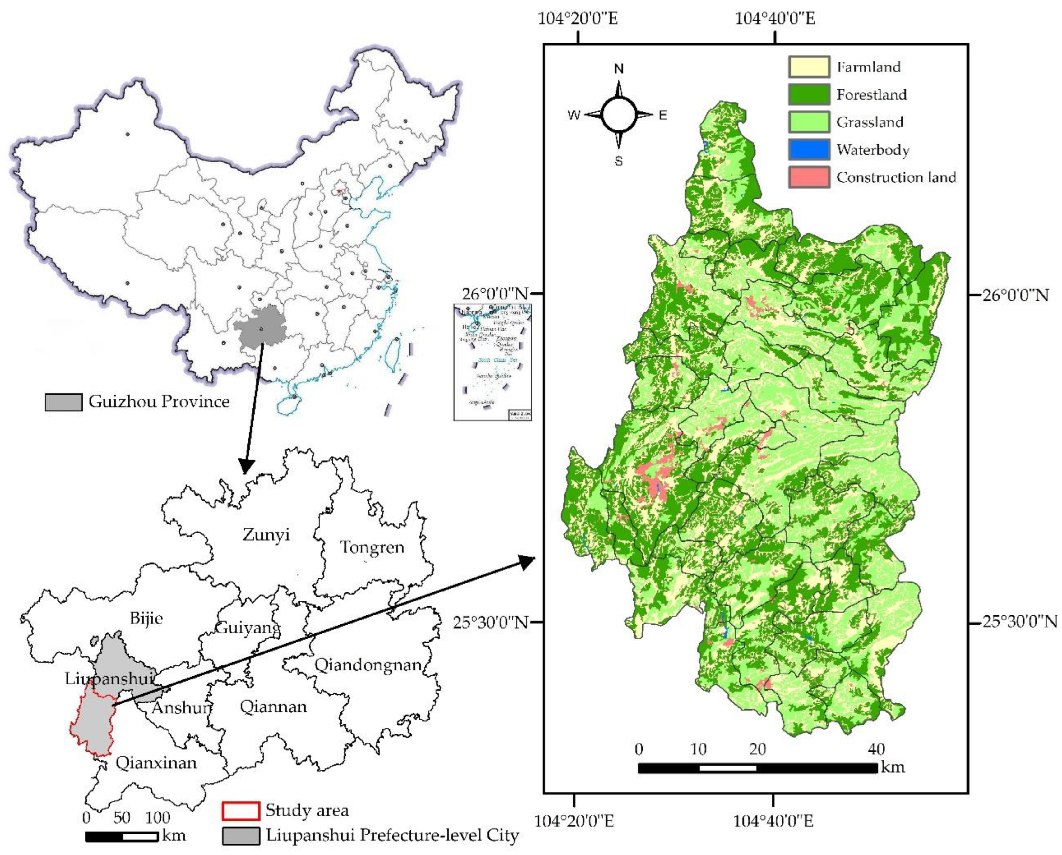
2.1. Study Area

At the junction of Yunnan and Guizhou, Panzhou city (104°17′–104°57′ E, 25°19′–26°17′ N) in western Guizhou Province is a part of Liupanshui prefecture-level city. As an important node for transportation, energy, commerce, logistics, and tourism between Yunnan Province and Guizhou Province, it has jurisdiction over six subdistricts, fourteen towns, and seven townships, with a total area of approximately 4057 km² (Figure 1). This area has a subtropical plateau monsoon climate with a mean annual temperature of 15.2 °C and an annual precipitation of 1390 mm. Panzhou city has karst landforms, with plateau mountains as the main body. The whole terrain is high in the northwest, low in the southeast, and uplifted in the central and southern parts. The forest coverage rate reaches 46.69%, with a dense distribution of rare animals and plants (e.g., millennium ancient ginkgo trees). There is a large coal reserve, accounting for 15% of the total coal reserve in Guizhou Province. However, due to the typical karst geomorphological characteristics, rapid urbanization and industrialization have made the ecological systems more fragile (e.g., soil erosion and rocky desertification), which has restricted regional development.

2.2. Data

The basic data of this study included the scenes of Landsat 8 OLI, digital elevation model (dem), net primary productivity (npp), normalized difference vegetation index, harmonized world soil database, annual precipitation data at 1 km resolution in China, and multi-period land-use land cover remote-sensing detection dataset in China. Land cover types were reclassified into farmland, forestland, grassland, waterbody, and construction land (Figure 1). All data (

Table 1. The types and sources of data.

Data Types	Data Sources	Resolution	Period
Landsat 8 OIL	The Geospatial Data Cloud (http://www.gscloud.cn, accessed on 2 September 2021)	30 m	2020
Digital Elevation Model	The Geospatial Data Cloud (http://www.gscloud.cn, accessed on 2 September 2021)	30 m	2020
Net Primary Productivity	Google Earth Engine, accessed on 8 September 2021	500 m	2014–2020
Normalized Difference Vegetation Index	Google Earth Engine, accessed on 8 September 2021	30 m	2020
Harmonized World Soil Database	The Food and Agriculture Organization of the United Nations (http://www.fao.org, accessed on 8 September 2021)	1 km
Annual precipitation data at 1 km resolution in China	The National Earth System Science Data Center (http://www.geodata.cn, accessed on 8 September 2021)	1 km	2014–2020
Multi-period land-use land cover remote-sensing detection dataset in China	The Resource and Environment Science and Data Central (https://www.resdc.cn/, accessed on 19 September 2021)	30 m	2020

) were represented, and raster data were uniformly resampled to 30 m for research purposes.

2.3. Methods

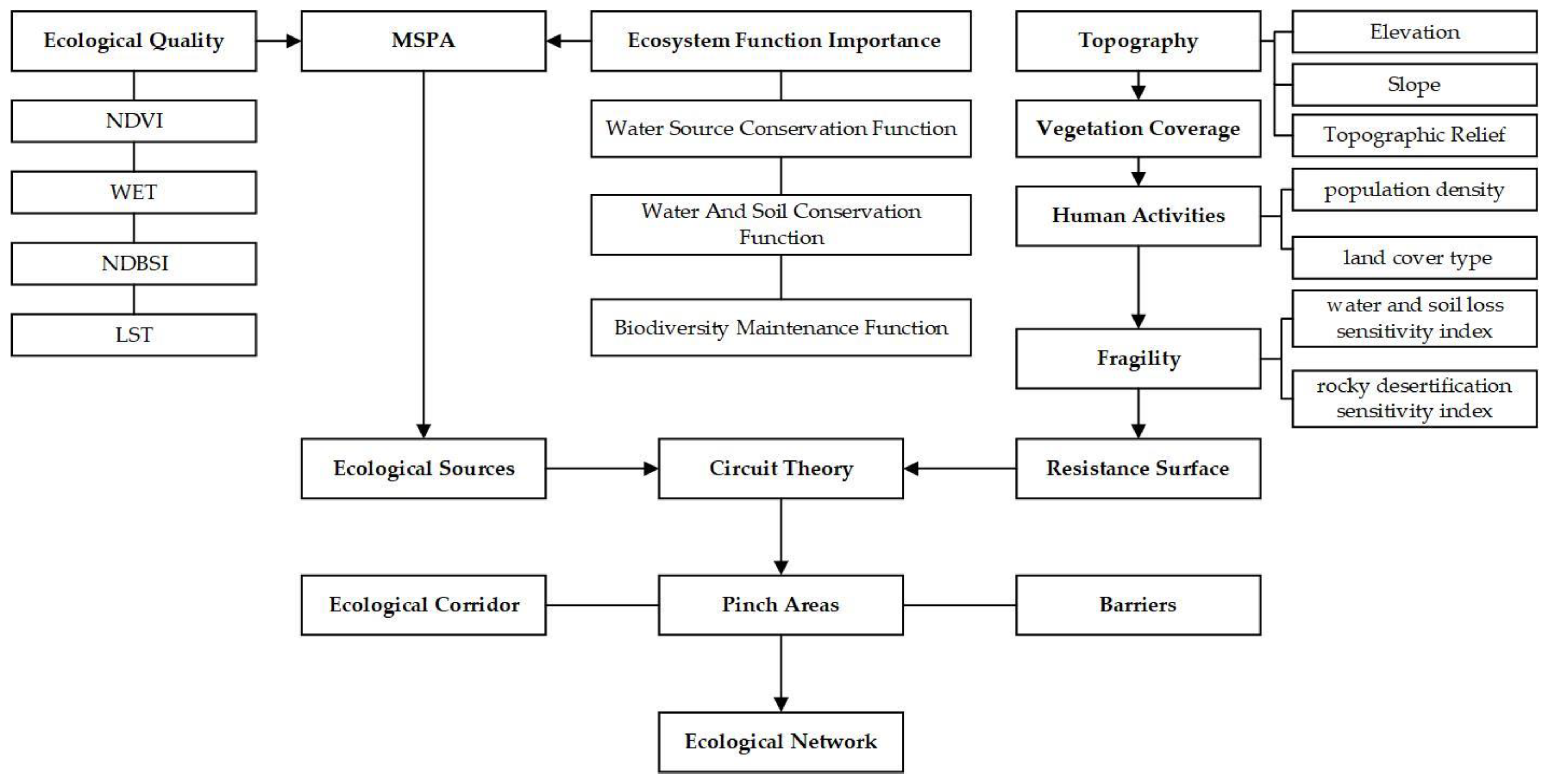
2.3.1. Research Framework

The overall research framework of this study can be divided into four steps (Figure 2):

Step 1: According to the ecological system in the study area, ecological quality (EQ) and ecosystem function importance (EFI) were evaluated. Combined with morphological spatial pattern analysis (MSPA), the ecological sources were determined.

Step 2: A comprehensive resistance surface was established based on the coefficient of variation method from four aspects: (1) topography of the study area; (2) vegetation status; (3) human activities; and (4) the soil erosion sensitivity index and the rocky desertification sensitivity index were introduced, both of which can analyze the ecological sensitivity of typical fragile ecological environment [42,43].

Step 3: Using circuit theory, the ecological corridors, ecological pinch areas, and ecological barriers were extracted based on the ecological source and comprehensive resistance surface.

Step 4: The initial ecological corridors were sorted and prioritized, and then patch verification was conducted to determine the protection order of ecological sources, pinch areas, and barriers, which were used as the basis for constructing the ecological security patterns and ecological restoration zones in the study area.

2.3.2. Assessment of EQ

Remote sensing has become an effective way to evaluate regional EQs [44,45]. It is not sufficient to adopt a uniform ecological index to assess ecological quality due to the complexity and diversity of the ecological system [46,47]. The remote sensing ecological index (RSEI), which integrates four indicators (greenness, wetness, dryness, and heat) through the principal component analysis (PCA) method [44,48,49], has been extensively applied to objectively evaluate eco-environmental quality without requiring manual parameter setting [44,50,51].

• Retrieval of the RSEI

Accordingly, the greenness indicator is represented by the normalized difference vegetation index (NDVI), which can manifest the environmental state in the RSEI. Meanwhile, the wetness indicator is measured by the wet component (WET) derived from the tasseled cap transformation. The indicator of dryness is estimated by the normalized differential build-up and bare soil index (NDBSI), composed of the index-based built-up index (IBI) and bare soil index (BI), and usually adopted to indicate the pressures generated from soil bareness and human activities on the environment. The land surface temperature (LST) is applied to indicate the heat indicator, which is selected as the indicator of local climate changes in response to environmental changes [51,52]. The formulas for those indicators were as follows [44,50,51]:

NDVI:

$$\mathrm{NDVI}=\left({\rho }_{\mathrm{nir}}-{\rho }_{red}\right)/\left({\rho }_{nir}+{\rho }_{red}\right)$$

(1)

WET:

$${\mathrm{Wet}}_{\mathrm{TM}}=0.0315{\rho }_{blue}+0.2021{\rho }_{green}+0.3102{\rho }_{red}+0.1594{\rho }_{nir}-0.6806{\rho }_{swir1}-0.6109{\rho }_{swir2}$$

(2)

$${\mathrm{Wet}}_{\mathrm{OLI}}=0.1511{\rho }_{blue}+0.1973{\rho }_{green}+0.3283{\rho }_{red}+0.3407{\rho }_{ }{}_{nir}-0.7117{\rho }_{swir1}-0.4559{\rho }_{swir2}$$

(3)

NDBSI:

$$\mathrm{IBI}=\frac{\frac{2{\rho }_{swir1}}{{\rho }_{swir1}+{\rho }_{nir}}-\left(\frac{{\rho }_{nir}}{{\rho }_{nir}+{\rho }_{red}}+\frac{{\rho }_{green}}{{\rho }_{green}+{\rho }_{swir1}}\right)}{\frac{2{\rho }_{swir1}}{{\rho }_{swir1}+{\rho }_{nir}}+\left(\frac{{\rho }_{nir}}{{\rho }_{nir}+{\rho }_{red}}+\frac{{\rho }_{green}}{{\rho }_{green}+{\rho }_{swir1}}\right)}$$

(4)

$$\mathrm{SI}=\frac{\left({\rho }_{swir1}+{\rho }_{red}\right)-\left({\rho }_{nir}+{\rho }_{blue}\right)}{\left({\rho }_{swir1}+{\rho }_{red}\right)+\left({\rho }_{nir}+{\rho }_{blue}\right)}$$

(5)

$$\mathrm{N}\mathrm{D}\mathrm{B}\mathrm{S}\mathrm{I}=(\mathrm{I}\mathrm{B}\mathrm{I}+\mathrm{S}\mathrm{I})/2$$

(6)

LST:

$$\mathrm{LST}=T/[1+(\lambda \times T/\rho )\ln \epsilon ]$$

(7)

$$T=K_2/\ln \left(K_1/L+1\right)$$

(8)

$$L=Gain\times DN+Bias$$

(9)

$$\epsilon =\{\begin{array}{l}0.995\hfill \\ 0.970\hfill \\ 1.0094+0.047\ln NDVI\hfill \\ 0.986\hfill \end{array}\begin{array}{c}\\ \\ \\ \end{array}\begin{array}{c}\mathrm{N}\mathrm{D}\mathrm{V}\mathrm{I}\le 0\\ 0<\mathrm{N}\mathrm{D}\mathrm{V}\mathrm{I}\le 0.157\\ 0.157<\mathrm{N}\mathrm{D}\mathrm{V}\mathrm{I}\le 0.727\\ \mathrm{NDVI}>0.727\end{array}$$

(10)

where ρ_blue, ρ_green, ρ_red, ρ_nir, ρ_swir1, and ρ_swir2 represent the reflectance of the blue band, green band, red band, near-infrared band, and shortwave infrared band1 and band2, respectively; λ is the wavelength of the emitted radiance (11.435 µm for Landsat 5/7 and 10.9 µm for band 10 of Landsat 8); ρ is a constant (1.438 × 10⁻² m K); K₁ and K₂ are calibration coefficients for TM/ETM+/OLI sensor thermal band, for TM, K₁ = 607.76 mW cm⁻²sr⁻¹µm⁻¹, K₂ = 1260.56 K, while for OLI, K₁ = 774.89 mW cm⁻²sr⁻¹µm⁻¹, K₂ = 1321.08 K; Gain and Bias are the band-specific multiplicative rescaling factor and the band-specific additive rescaling factor, respectively, which are available in the head file of the used image; and DN represents the digital number of a given pixel.

2.

Acquisition of the RSEI

The four indicators, i.e., NDVI, WET, NDBSI, and LST, were integrated into the RSEI via PCA. According to the load of each indicator on the RSEI, the contribution of each indicator was weighted. This method avoids losing original information and explains most of the total variation in the dataset. The component of PCA, was employed to represent the RSEI. As such, the expression of RSEI can be written as follows [46,53]:

$${\mathrm{RSEI}}_0={\displaystyle \sum _{i=1}^n{\omega }_i\times P{C}_i[f(\mathrm{NDVI},\mathrm{WET},\mathrm{NDBSI},\mathrm{LST})]}$$

(11)

$$\mathrm{R}\mathrm{S}\mathrm{E}\mathrm{I}=\left(\mathrm{R}\mathrm{S}\mathrm{E}{\mathrm{I}}_0-\mathrm{R}\mathrm{S}\mathrm{E}{\mathrm{I}}_{\min }\right)/\left(\mathrm{R}\mathrm{S}\mathrm{E}{\mathrm{I}}_{\max }+\mathrm{R}\mathrm{S}\mathrm{E}{\mathrm{I}}_{\min }\right)$$

(12)

where RSEI₀ is the result calculated by PCA; n is the number of the extracted components. If the cumulative percentage of eigenvalues is greater than 80%, the corresponding principal components are extracted. ω_i is the weight of the principal component i, which is automatically assigned by the contribution rates of each eigenvalue; PC_i is the principal component i, which is the weighted sum of NDVI, WET, NDBSI, and LST, according to the contribution of each factor to the principal component i; RSEI_min and RSEI_max are the minimum and maximum values of RSEI₀ in the study area, respectively. Before using PCA, the values of the four indicators were normalized between 0 and 1 to eliminate the impact of the unit. The PCA was then calculated in ENVI (version 5.3) software using the PCA Rotation tool; as a result, a single-band image (i.e., RSEI₀ image) was created. Subsequently, the RSEI was divided into five levels, each with a 0.2 increment, i.e., Level 1 (poor): 0–0.2, Level 2 (fair): 0.2–0.4, Level 3 (moderate): 0.4–0.6, Level 4 (good): 0.6–0.8, and Level 5 (excellent): 0.8–1. Of the five levels, Level 1 represented a very bad condition of EQ, and Level 5 denoted an excellent EQ condition [46,54].

2.3.3. Assessment of the EFI

The EFI of the study area was quantitatively analyzed to provide a basis for ecological security patterns and ecological restoration. According to the concept and method in the ‘Guidelines for the Delimitation of the Red Line of Ecological Protection’ of China [55], the ecological functions of the study area were classified into three types: the water source conservation function (WR), water and soil conservation function (A_c), and biodiversity maintenance function (Q_xj). Therefore, the EFI was obtained from the three types of ecological functions (WR, A_c, and Q_xj): WR was calculated by the NPP quantitative index evaluation method [56], A_c was assessed mainly by the revised universal soil loss equation (RUSLE) [57,58], and Q_xj was computed by the Habitat Quality (HQ) module in InVEST software [59]. The formulas of those indicators were as follows:

WR:

$$\mathrm{WR}=NP{P}_{\mathrm{m}ean}\times F_{sic}\times F_{pre}\times \left(1-F_{slo}\right)$$

(13)

where NPP_mean is the average NPP of ecosystems in the study area from 2000 to 2020; F_sic is the capacity factor of the soil seepage, and the value for each soil type was shown in Appendix A.1 of Appendix A; F_pre is the average precipitation factor from 2014 to 2020 in study area; and F_slo is the slope of the study area.

A_c:

$${\mathrm{A}}_{\mathrm{c}}=A_p-A_r=R\times K\times L\times S\times (1-C)$$

(14)

where A_p is the potential soil erosion; A_r is the actual soil erosion; R is the factor of average precipitation erosivity from 2000 to 2020; K is the factor of soil erodibility in the study area; and L, S, and C represent the slope length, slope, and vegetation cover, respectively. The detailed calculations of the parameters in A_c are presented in Appendix A.2 of Appendix A.

Q_xj:

$${\mathrm{Q}}_{\mathrm{xj}}=H_j\left(1-\left(\frac{D_{xj}^z}{D_{xj}^z+k^z}\right)\right)$$

(15)

where Q_xj is the HQ index of grid x in land-use type j; D_xj is the habitat stress level of grid x in land-use type j; H_j is the habitat suitability of land-use type j; k is the half-saturation constant, usually set to 0.5 in the InVEST model; and Z is a normalized constant, for which the default parameter of the InVEST model was 2.5. More details can be seen in the user’s guide of the InVEST Model [59], and the relevant parameters are presented in Appendix A.3 of Appendix A.

Based on the evaluation results of three kinds of ecological functions (WR, A_c, and Q_xj), the total value of the EFI was shown as follows:

$$\mathrm{EFI}=\mathrm{WR}+{\mathrm{A}}_{\mathrm{c}}+{\mathrm{Q}}_{\mathrm{xj}}$$

(16)

The comprehensive evaluation of the EFI was normalized and separated into five levels based on natural breaks: Level 1 (0.0–0.25, low), Level 2 (0.25–0.37, comparatively lower), Level 3 (0.37–0.47, median), Level 4 (0.47–0.58, comparatively higher), and Level 5 (0.58–1.0, high).

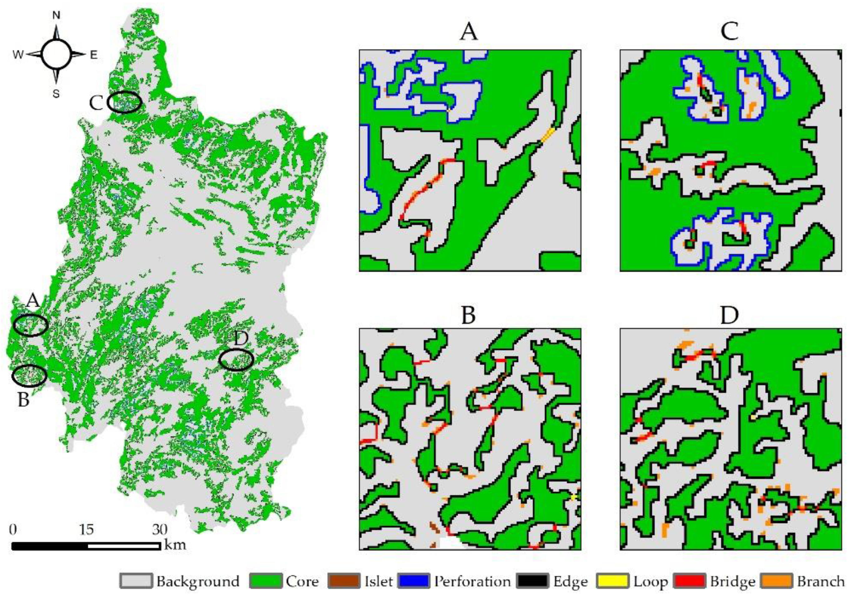
2.3.4. Landscape Pattern Analysis Based on MSPA

MSPA, proposed by Vogt [60], analyses landscape patterns by combining the mathematical morphology research of Riitters [61] with a mathematical morphology-mapping algorithm developed by Soille [62]. Hence, the MSPA method not only can unveil geometric descriptions and patch associations but also identify spatial pattern classes of landscapes at the pixel level with connectivity importance and specific ecological meaning (Appendix A.4 of Appendix A).

Depending on land-use data with a 30 m × 30 m spatial resolution for Panzhou, forestland was set as the foreground in the MSPA method, while other land cover types (farmland, grassland, waterbody, and construction land) were set as the background. Then, using the eight-neighborhood analysis method and the Guidos Toolbox software 3.0 (https://forest.jrc.ec.europa.eu/en/, accessed on 31 May 2022) [62], the edge width parameter was set to 1 (a reference to the radius of a circle with an area of 1 hectare), and the particle size was set to 30 m for MSPA.

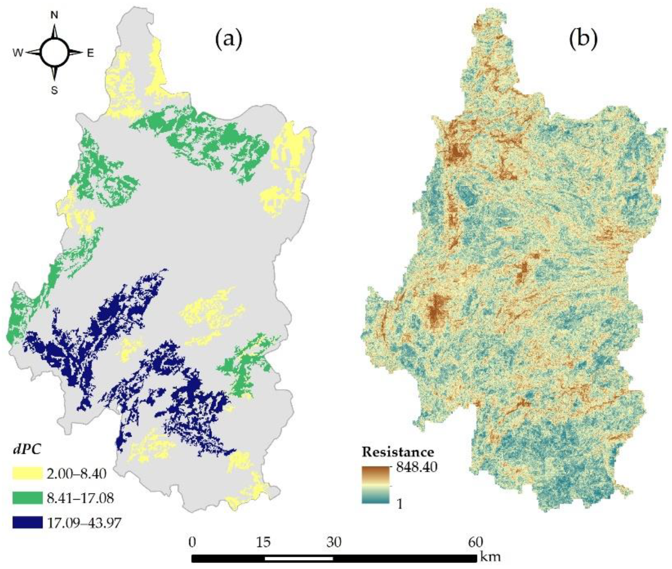
2.3.5. Selection of Ecological Sources

Ecological sources, as the basis for the construction of ecological networks, aim to improve ecological quality, protect important habitats, and stabilize regional ecosystem services to a certain extent [63]. According to the results of the RSEI, EFI, and MSPA, high levels of areas within RSEI > 0.8 and EFI > 0.58 were applied to the initial ecological sources because these areas were of high suitability and functionality. Subsequently, the core areas were used to merge into the initial ecological sources. Considering that patches in the initial ecological sources with a small area are not ecologically suitable, these patches with an area of less than 5 km² were eliminated from the initial ecological sources. Finally, to maintain the continuity and integrity of the preserved patches, the probabilistic connectivity index (PC) was used to analyze the connectivity of ecological sources [64,65,66]. The formulas for PC calculation are as follows:

$$\mathrm{PC}=\frac{{\displaystyle \sum _{i=1}^n}{\displaystyle \sum _{j=1}^n}{\mathrm{a}}_{\mathrm{i}}\times {\mathrm{a}}_{\mathrm{j}}\times P_{ij}^{\ast }}{A^2}$$

(17)

$$dPC=100\%\cdot \frac{\mathrm{PC}-{\mathrm{PC}}_{\mathrm{remo}}}{\mathrm{PC}}$$

(18)

where n is the total number of patches in the ecological sources; a_i and a_j are the areas of patch i and patch j, respectively; A is the total landscape area; and $P_{ij}^{\ast }$ is the greatest possibility of the direct diffusion of species in patches i and j. PC_remo is the overall index of the remained patches after removing patch i; dPC is the variation in PC. The higher dPC is, the more importance the patch has and can be retained. Conefor Sensinode 2.6 software (http://www.conefor.org, accessed on 31 May 2022) was used to calculate the PC values.

2.3.6. Construction of Resistance Surface

A resistance surface is a key link in the construction of an ecological network, and the value can reflect the difficulty of passing through the ecological process. In this study, the resistance surface was constructed from four perspectives: (1) topographic factors, including elevation, slope, and topographic relief (see Equation (A3) in Appendix A.2); (2) vegetation coverage (see Equation (A4) in Appendix A.5) [67]; (3) population density and land cover type, which reflect regional human activities; and (4) the water and soil loss sensitivity index (see Equation (A5) in Appendix A.5) [68] and the rocky desertification sensitivity index (see Equation (A6) in Appendix A.5). Each resistance factor was divided into five levels according to the natural breakpoint method. The resistance coefficients were assigned 1, 250, 500, 750, and 1000, and the weight of each resistance factor was determined by the coefficient of variation weight method [69]. The calculation of resistance factors and the coefficient of variation method are presented in Appendix A.5 of Appendix A. The resistance coefficient and its weight are shown in

Table 2. Resistance coefficient and weight of each resistance factor in Panzhou city.

RC	Elevation	Slope	TR	VC	PD	LCT	WSLSI	RDSI
Weight	0.078	0.102	0.108	0.102	0.283	0.108	0.088	0.131
1	752–1563	0–10.4	20–104	0.83–1	19.12–293.18	Forestland	0–0.25	0–0.15
250	1563–1751	10.4–17.83	104–151	0.64–0.83	293.18–822	Waterbody	0.25–0.36	0.15–0.29
500	1751–1931	17.83–25.87	151–206	0.44–0.64	822–1864.63	Grassland	0.36–0.49	0.29–0.43
750	1931–2178	25.87–36.09	206–287	0.19–0.44	1864.63–3970.46	Farmland	0.49–0.6	0.43–0.58
1000	2178–2867	36.09–75.17	287–670	0–0.19	3970.46–7997.61	Construction land	0.6–1	0.58–1

RC: resistance coefficient; TR: topographic relief; VC: vegetation coverage; PD: population density; LCT: land cover type; WSLSI: water and soil loss sensitivity index; RDSI: rocky desertification sensitivity index.

.

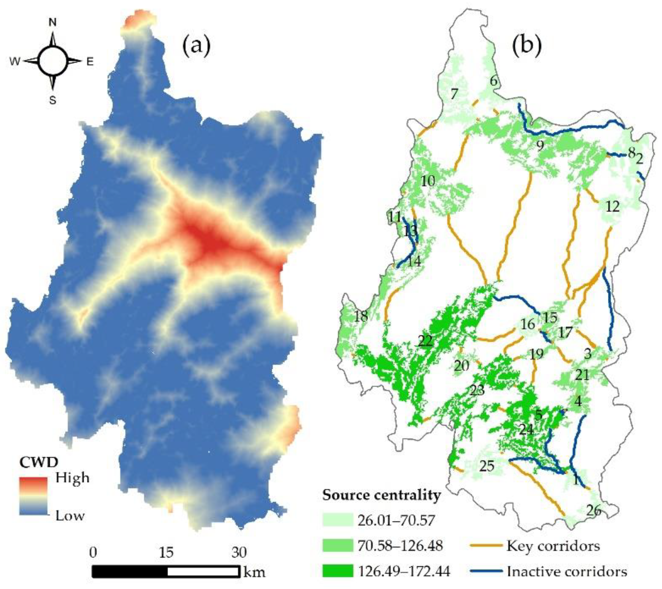
2.3.7. Circuit Theory

Circuit theory simulates the process of species migration or energy flow in the ecological process by using the electronic random walk phenomenon in the field of physics [16]. It identifies the ecological corridor by constructing the minimum cost path between the ecological source and the ecological resistance surface [70]. In this study, the Linkage Mapper (LM) model of GIS (https://circuitscape.org, accessed on 31 May 2022) was applied to identify the key ecological corridors and inactive ecological corridors, in which the ecological sources were paired. Then, the minimum cost path between each pair of ecological sources was identified according to the initial minimum cost path method. Finally, the minimum cost path passing through other ecological sources was removed to generate the ecological corridor [71].

The importance of an ecological source in the ecological security pattern can be described in terms of the source centrality by applying Centrality Mapper (CM) in the LM model. Referring to the circuit theoretical model, CM regards the minimum cost-weighted distance (CWD) between any two ecological sources as a resistance. It turns the current into different ecological sources and accumulates the currents successively to obtain the cumulative current value of each corridor [50]. Higher current values indicate better connectivity of that ecological source in the ecological security pattern. Similarly, based on the Pinchpoint Mapper tool in the LM model, pinch areas can be discerned, through which all currents (species) must pass [71]. Such areas can represent species migration with the highest density, and thus the protection of pinch areas should be prioritized in ecological protection [50]. Conversely, barrier points, defined as nodes with a relatively high current density and large ecological resistance value in ecological corridors, can be identified by the Barrier Mapper tool in the LM model. Such points reflect the key areas that hinder the flow of ecosystem services and need to be removed to improve landscape connectivity [70]. Barrier points are extracted with a high improvement coefficient (IC), which is defined as the restoration value of connectivity per unit distance. In this study, the search radius in the Barrier Mapper tool was set to 150 m, and the moving window method (diameter D) was used to identify barrier points.

3. Results

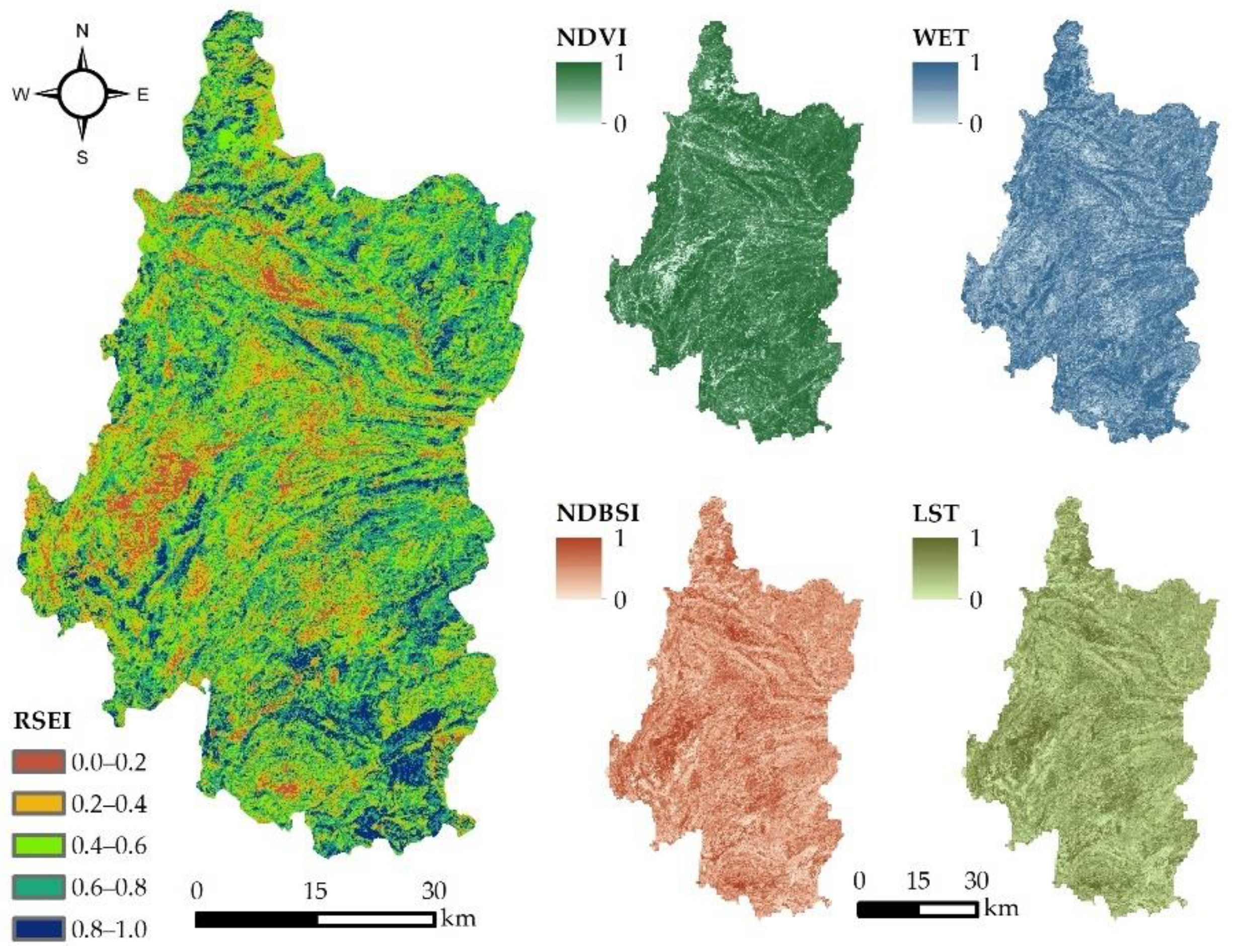
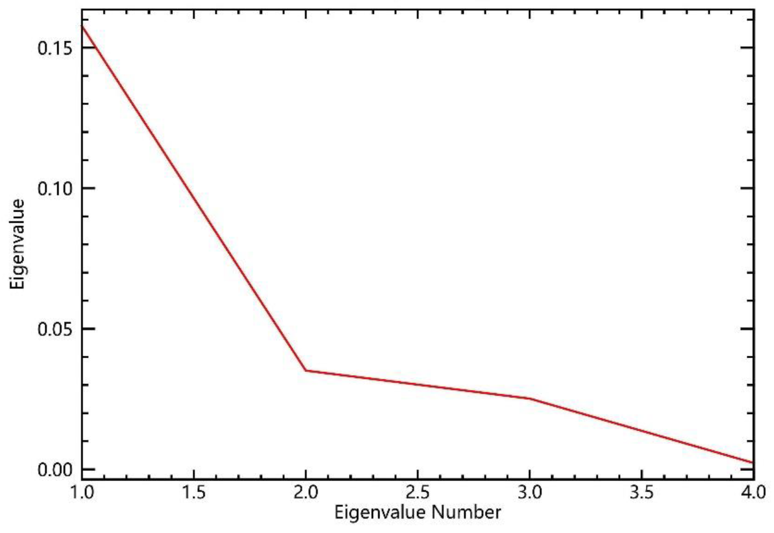
3.1. Distribution of the RSEI

The RSEI is a spatially continuous measure of EQ that couples four indicators into one by PCA [46]. The PCA data for the RSEI of Panzhou city are shown in

Table 3. Principal component analysis of four indicators.

Indicators	PC1	PC2	PC3	PC4
NVDI	0.448	0.570	−0.550	0.415
WET	0.555	−0.147	0.663	0.481
NDBSI	−0.545	−0.290	−0.165	0.769
LST	−0.440	0.755	0.481	0.076
Eigenvalues	0.158	0.035	0.025	0.002
Percent covariance eigenvalue (%)	71.62%	15.94%	11.42%	1.02%

and Figure A1. PC1 had the largest eigenvalue among the four PCs, with a proportion of approximately 71%, while PC2 had the second-largest eigenvalue (approximately 15.94%). The total proportion of PC1 and PC2 exceeded 80%, which indicated that PC1 and PC2 could represent and gather more information than PC3 and PC4 on the four indicators. In PC1, the NVDI and WET had opposite signs; that is, they had a positive impact on EQ. Nevertheless, the NDBSI and LST were negative in PC1, indicating that they had a negative impact on EQ. Therefore, according to the PCA results, the final value of the RSEI was calculated with the weighted sum of PC1 and PC2, in which the weights were assigned by the contribution rates of each eigenvalue [51,53].

Figure 3 shows the spatial distribution of the RSEI, which is divided into five levels. The spatial distribution of the RSEI in Panzhou was apparently dispersed due to the fragmented landscape of Wumeng Mountain. The EQ was poorer in the western areas than in the peripheral areas close to the rural zone, with the red and yellow polygons concentrated in the western areas. Level 1 (0.0–0.2, poor) occupied an area of 305.45 km², accounting for 7.53% of the total study area. This level was mainly distributed in the western region, which was the core area of construction land, e.g., cities and industrial and mining areas. Because of urban expansion and intensive human activities in the west, the NDVI and WET were lowest, while the NDBSI and LST values were higher. Level 2 (0.2–0.4, fair) covered an area of approximately 683.28 km² (16.85%), which was dominated by rural construction land and less farmland near rural settlements with a lower HQ. Level 3 (0.4–0.6, moderate) covered an area of 1210.64 km² (29.85%), mainly including waterbodies and high-coverage farmlands with a medium HQ. Level 4 (0.6–0.8, good) was distributed in the transition zone between construction land and moderate-vegetation mountains due to the lower intensity of human activity, with an area of approximately 1354.87 km², accounting for 33.40% of the total study area. Level 5 (0.8–1.0, excellent) was mainly scattered in the northern and southern areas with high-vegetation mountains, covering an area of 501.77 km² (12.37%). This result was consistent with the highest values of the NDVI and WET and the lowest values of the NDBSI and LST due to the implementation of ecological-protection policies. In general, the distribution of RSEI was relatively fragmented and gradually increased as it moved away from the central urban area. This characteristic showed that improving EQ requires ecological restoration in urban areas and ecological conservation in high-vegetation coverage areas.

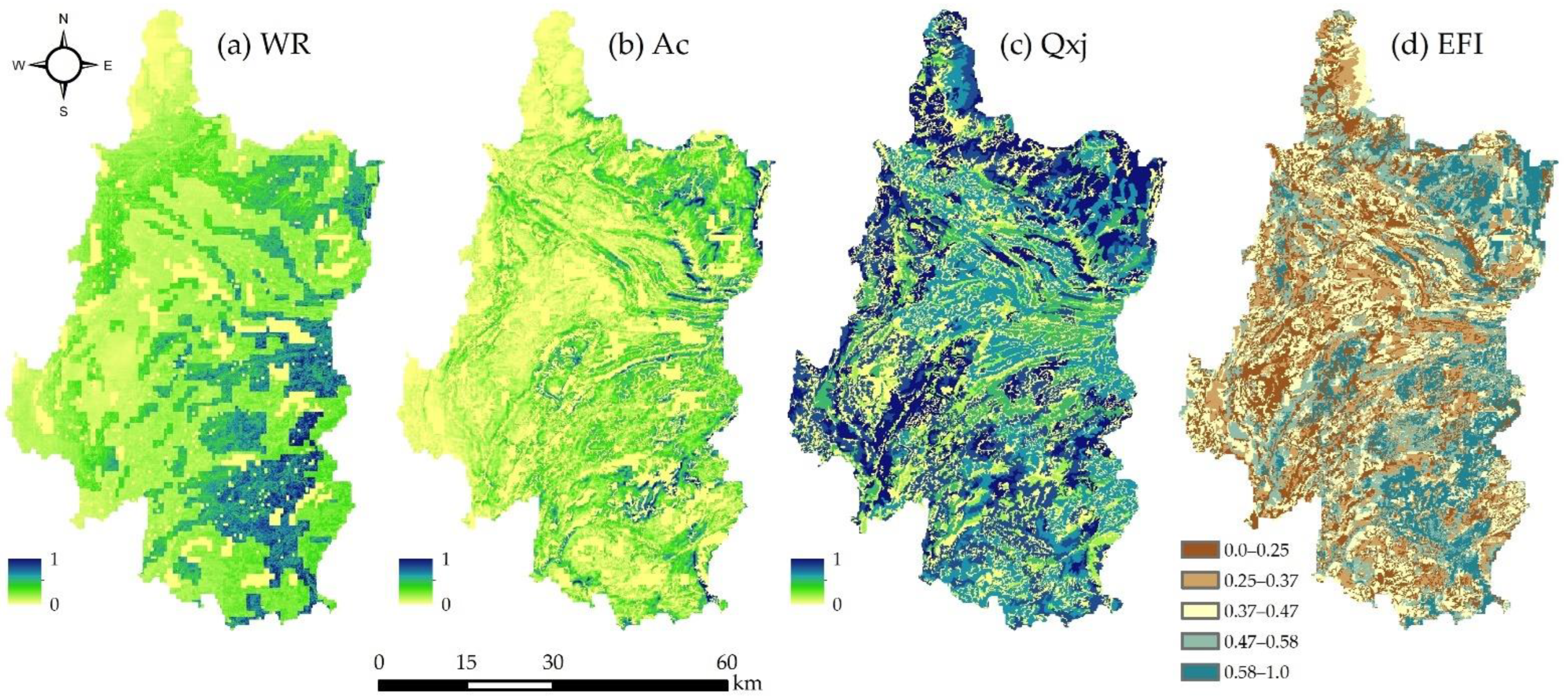
3.2. Distribution of the EFI

Ecosystem service functions based on the natural conditions in Panzhou city were evaluated and normalized between 0 and 1 (Figure 4a–c). The larger the value of the indicator was, the more important the function was. Areas with high values of the water conservation function were primarily concentrated in the east because of high amounts of vegetation and slight anthropogenic disturbance (Figure 4a). Moreover, this distribution of such areas was in accordance with the characteristics of precipitation; that is, the precipitation decreased from southeast to northwest, and the southeast region had relatively more precipitation. Nevertheless, the distribution of a low value of the water and soil conservation function was relatively dispersed, indicating that soil erosion was prone to occur in these areas. Meanwhile, areas with high values were scattered in the north-eastern and south-eastern regions (Figure 4b). In terms of the biodiversity maintenance function (Figure 4c), the northern and southwestern parts of the study area were relatively important in biodiversity maintenance, where there were national scenic spots and the largest natural grassland in southwestern China with an extreme abundance of animal and plant resources.

The comprehensive evaluation of the EFI was obtained by the superposition of single function evaluation results, and then it was normalized and separated into five levels based on natural breaks (Figure 4d). The importance levels, i.e., Level 4 and Level 5, covered large areas of the eastern region, with about 35% of the studying area. Level 1 (0.0–0.25, low) dominated an area of 954.71 km², accounting for 23.54% of Panzhou city, and Level 2 (0.25–0.37, comparatively lower) occupied an area of 641.69 km², accounting for 15.82%, and was mainly distributed in the western part of the study area. Such areas had relatively dense populations and put extreme pressure on ecological protection. Level 3 (0.37–0.47, median) covered 1022.59 km² (25.21%), which was associated with the location of farmland and grassland. Level 4 (0.47–0.58, comparatively higher) and Level 5 (0.58–1.0, high), with areas of 852.10 km² (21.01%) and 584.91 km² (14.42%), respectively, were distributed in eastern Panzhou city. These two levels performed relatively important ecological functions and played an important role in the sustainable development of the ecological environment.

3.3. Analysis of Landscape Patterns Based on MSPA

As shown in

Table 4. Results of MSPA in Panzhou city.

Categories	Area (km2)	Proportion (%)
Core	1306.55	82.65
Islet	0.05	0.00
Perforation	33.25	2.10
Edge	230.22	14.56
Loop	0.19	0.01
Bridge	1.79	0.11
Branch	8.7	0.55

and Figure 5, the core area of Panzhou city was 1306.55 km², accounting for 82.65% of the foreground area. It was mainly concentrated in the northern and western regions, indicating that it had strong connectivity. However, the core areas were less abundant in the central region, where the spatial connectivity was poor and the environment was not conducive to the flow of material and energy. The edge areas were 230.22 km², accounting for 14.56% of the foreground area, which could better reduce the interference caused by the transfer from the external landscape to the core area. The islets were distributed in the upper reaches of rivers, occupying 0.05 km² (Figure 5B). Although small in size, they could be used as ecological stepping-stones to facilitate the flow of material and energy in the region. The perforation areas occupied 33.25 km², accounting for 2.10% of the foreground area, and played a better role in the edge effect. The loop areas were shortcuts for animal movement within the patches and facilitated the migration of species within the same patches [25], occupying 0.01% of the foreground area (Figure 5A). The bridge areas that have essential ecological significance for species migration and diffusion were 1.79 km², accounting for 0.11% of the foreground area. Such areas with a relatively small proportion demonstrated that the material and energy flows inside the core area were hindered. The branches were considered interruptions of corridor connections with some connectivity, accounting for 0.55% of the foreground area in Panzhou city (Figure 5C,D). Overall, the core areas in the study area were concentrated in the north, south, and west, indicating that the habitat and environment were suitable for species activities in these areas.

3.4. Ecological Source Identification and Resistance Surface Construction

The dPC value was calculated, and patches with a dPC less than 2 were removed. A total of 26 patches were identified as ecological sources. The total area of the ecological sources was 1007.74 km², accounting for 24.84% of the study area. Using the natural breaks, the ecological sources were divided into three classes, in which higher values indicated more important locations, as shown in

Table 5. Statistics of the ecological sources.

Value	Number	Total Area (km2)	Area Percentage
dPC ≥ 17.09	3	328.18	32.57%
17.08 ≥ dPC ≥ 8.41	5	318.62	31.62%
dPC ≤ 8.40	18	360.95	35.82%

and Figure 6a. The number of patches where the dPC was greater than 17.09 was low, indicating that a few patches in the study area significantly impacted the overall connectivity relative to the patches where the dPC was less than 8.40. In terms of land cover types, most of the ecological sources were composed of forestland, grassland, and water bodies. Among them, the forestland type sources were concentrated in the northern, western, and south-eastern regions of the study area, including the state-owned Forest Farm of Dengjiawan and the state-owned Forest Farm of Bajiaojing and Niangniang Mountain. The grassland-type sources were mainly located in the northern region, that is, the Wumeng Prairie and the Poshang Prairie. The water area type sources were distributed in the south, which is a tributary of the Nanpan River of the Pearl River system.

The resistance surface constructed by combining resistance factors (Table 2) reflected the disturbance that species would experience during their migration between ecological sources. Among the eight resistance factors (Table 2), the population density factor with the highest weight (0.283) affected the migration of species in two aspects: one was to exert pressure on the environment through the high-intensity construction and development of nature that destroyed the living conditions of species, and the second was the frequent human activities that interfered with the activities of species. Moreover, the rocky desertification sensitivity index has a relatively higher impact on the connectivity between ecological sources. The higher the value of this index was, the greater resistance of this index to living activities.

The resistance values for the resistance surface in Panzhou city ranged from 1 to 848.40 (Figure 6b). The high-resistance areas in the western region presented a flaky distribution, most of which were occupied by cities and settlements, and the values were gradually reduced outward from cities and settlements. The low-resistance areas in most of the study area appeared distributed and fragmented but were concentrated in the southern region. The center of the study area was represented by high mountains and hills that became high-value resistance areas. This was mainly affected by ecological projects in Panzhou city, such as the policy of ‘Low Production Forest Improvement’, ‘Law of Soil and Water Loss Control’, and the program of Grain for Green, which made the ecological function and biomass of forest in mountainous areas raise effectively and the obstacle to biological flow significantly weaken. In the future, it is essential to strengthen the maintenance and construction of the ecological landscape in the region to improve the ecological flow.

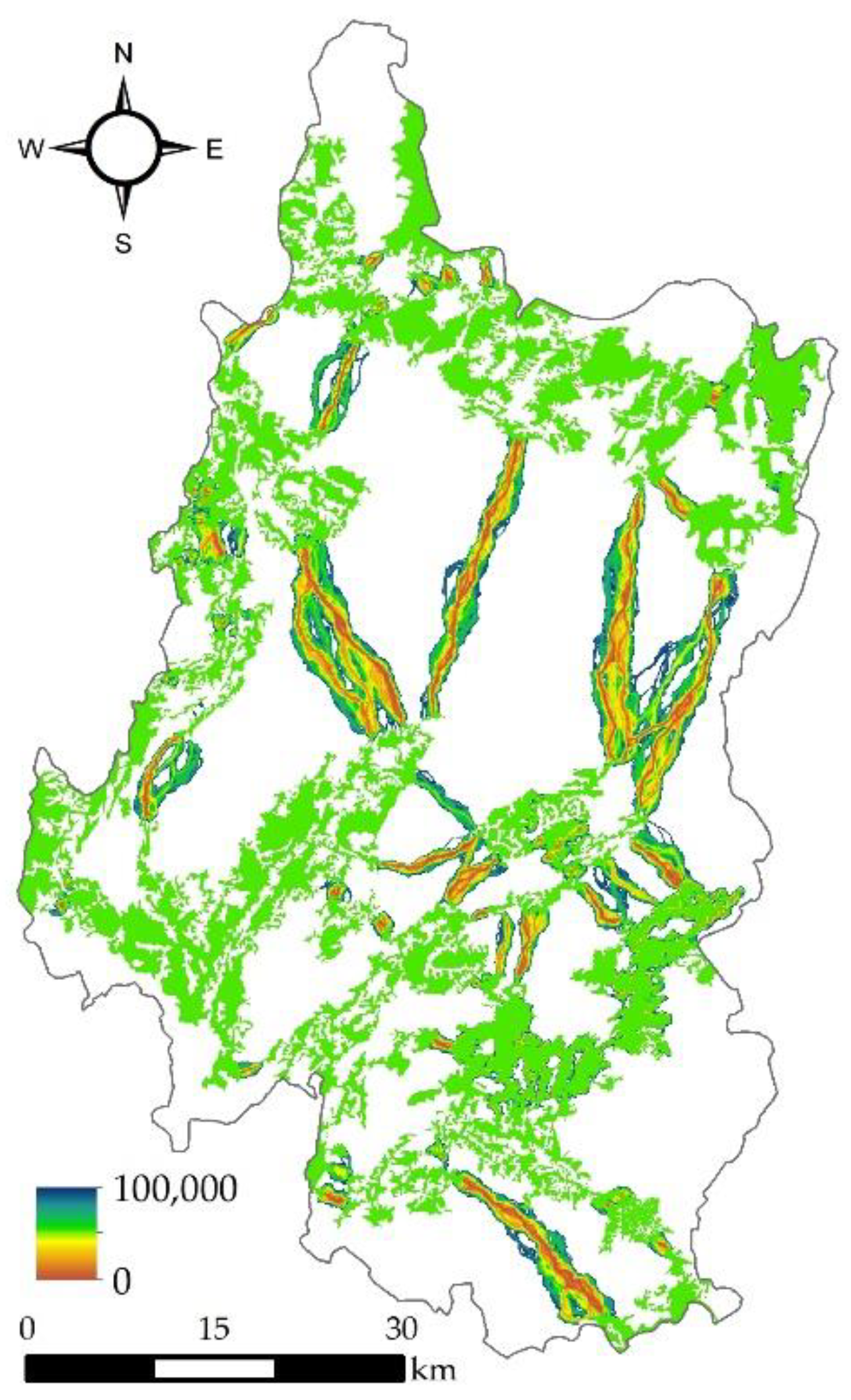
3.5. Distribution of Ecological Corridors

In this study, according to the ecological sources and ecological resistance surface, the minimum cost-weighted distance, source centrality, and ecological corridors were calculated based on circuit theory (Figure 7). The value of the minimum cost-weighted distance indicated the difficulty of source expansion from low to high (Figure 7a). Due to being far from the ecological sources, the high-value CWD was concentrated in the central part of Panzhou city and decreased outward. On the contrary, CWD was relatively small in the north, west, and south of the study area. This meant that the high-value CWD in the middle made the ‘North–South’ biological flow channel blocked or difficult and was not conducive to the species migration and energy exchange in the whole region.

The source centrality of 26 ecological sources ranged from 26.01 to 172.44 (Figure 7b). All ecological sources were divided into three levels, among which the darker the ecological source was, the stronger the centrality was. On the whole, the centrality of the ecological sources in the southern area was generally higher than that of the northern area. The centrality value of the No. 23 ecological source was the highest, illustrating that this patch was covered by forest and contributed the most to the connectivity of regional ecological sources. In contrast, the minimum value of centrality was found for the No. 26 ecological source, which was located in the south of the study area near the administrative boundary. At the same time, it was reflected that the centrality values of the small sources (i.e., No. 3, 4, 15, 16, 17, 19, and 21) were not high, although they were concentrated in terms of spatial distribution. This might arise from the smaller areas and comparative fragmentation of these sources, both of which weakened the biological flow between the sources and their surrounding patches.

Ecological corridors are the basic framework for maintaining regional ecological security by connecting different sources, increasing regional landscape connectivity, and maximizing ecological benefits [72]. A total of 63 ecological corridors, composed of 45 key ecological corridors and 18 inactive ecological corridors, were extracted from the least-cost path (LCP) via Linkage Mapper (Figure 7b). The total length of the key ecological corridors was 203.12 km, with an average of 4.51 km, while the maximum length was 25.32 km, and the minimum was 0.03 km. The key ecological corridors with lengths greater than 10 km, accounting for 6 and 126.87 km, were densely concentrated in the central part where the minimum cost-weighted distance was located. Such corridors formed a series of north–south orientation ecological channels, connected the ecological sources of the Niangniang Mountains and Wumeng Prairie, and maintained ecological security in the central part. There were 17 key corridors with a length of 1–9 km, accounting for 70.22 km, and 22 key corridors with a length of less than 1 km. The shorter key ecological corridors were mainly located in the periphery area, connecting some small and close ecological sources. The ecological sources (No. 3, 15, 16, 17, 19, and 21) in the south-eastern area were mainly connected by overlapping key corridors, indicating that species movement in this area was frequent. In addition, the total length of inactive ecological corridors was approximately 163.31 km (an average of 9.07 km with a maximum of 30.86 km and a minimum of 0.45 km). The longer inactive corridors connected the ecological sources with a larger area. The inactive corridors can be protected as backup resources for regional ecological security. Therefore, the measures of ecological restoration, such as forest construction projects and shelter forest projects, should be implemented to expand the area of ecological sources and improve the connectivity of ecological sources in Panzhou city.

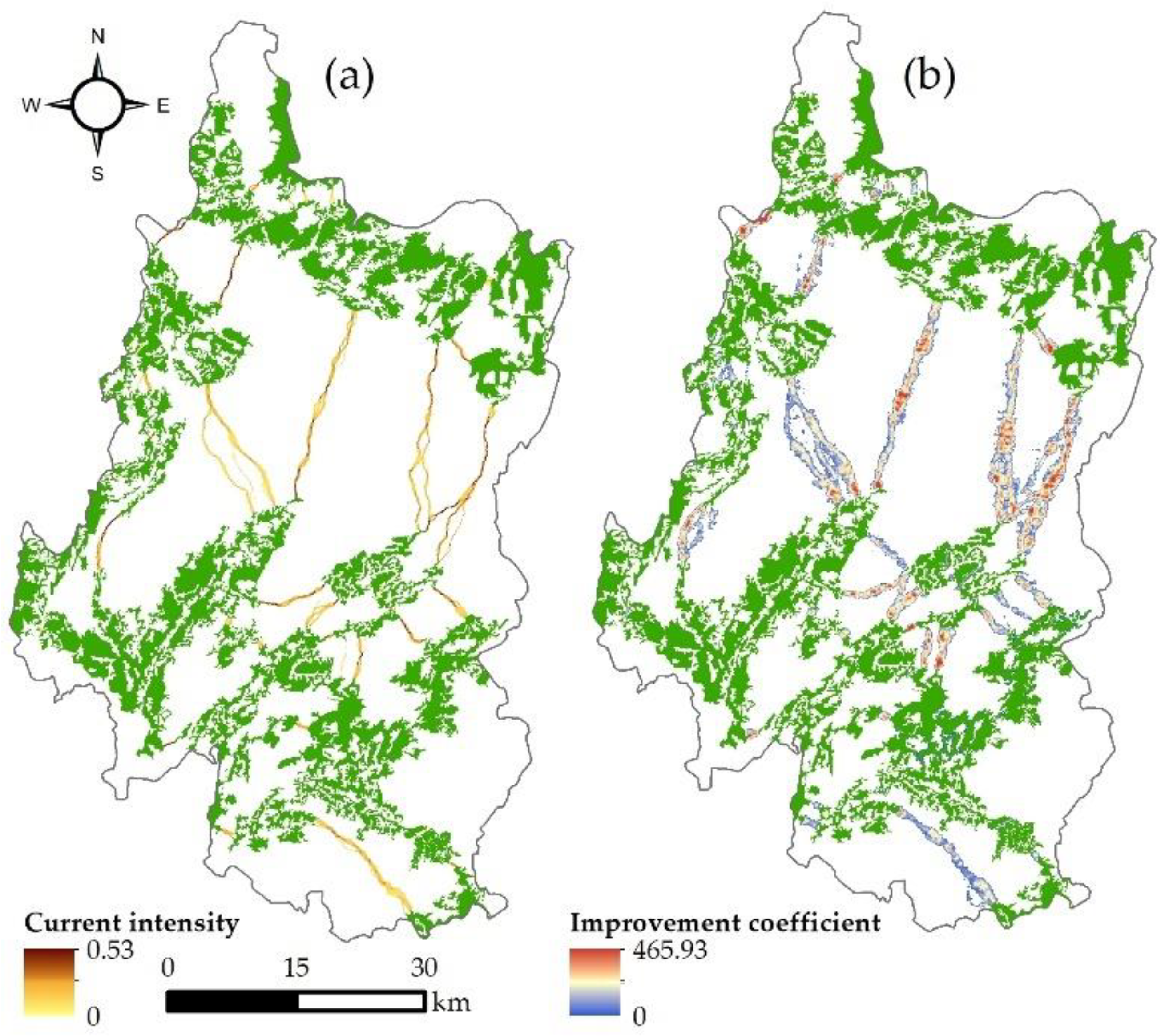
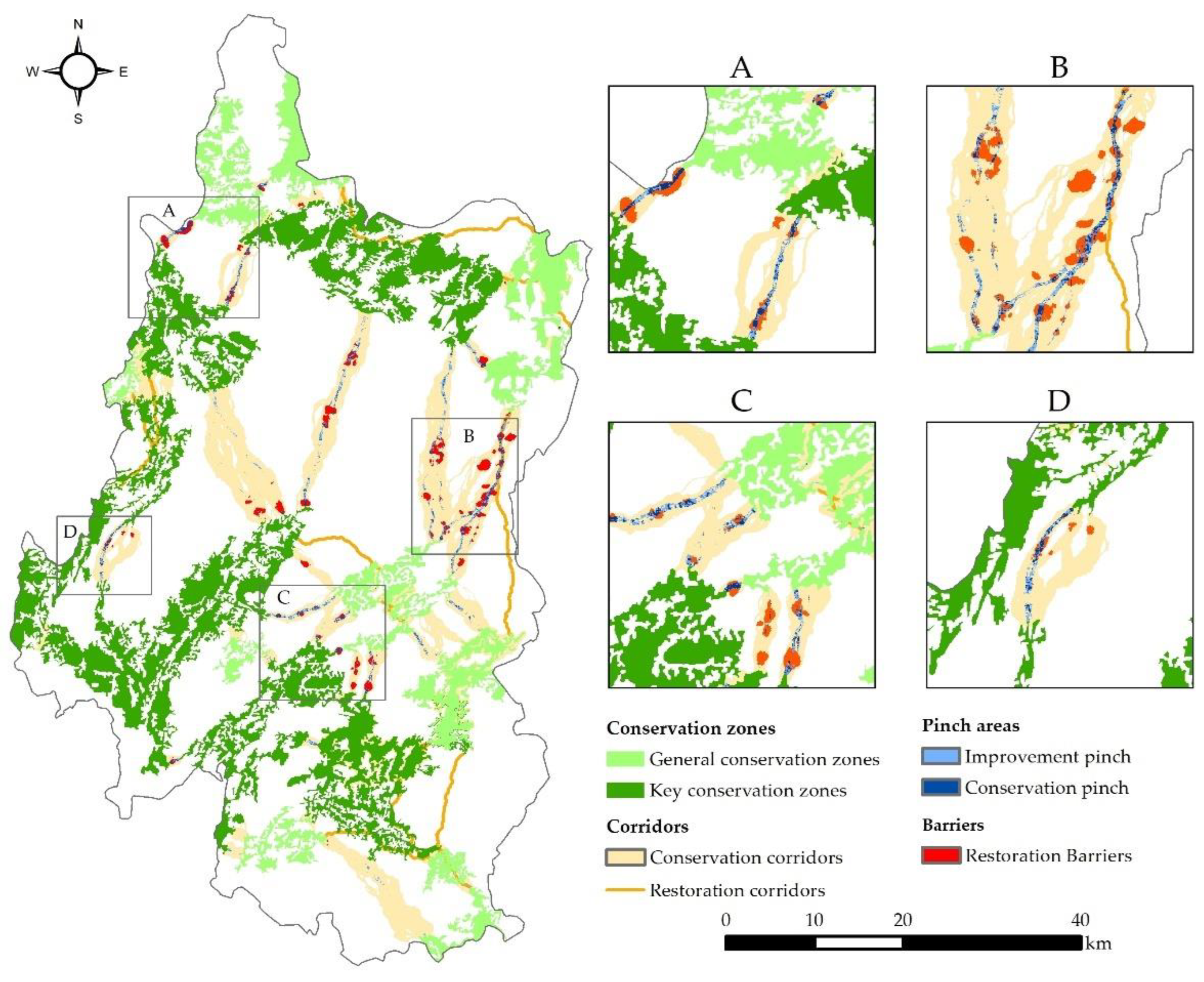
3.6. Identification of Pinch Areas and Barriers

Pinch areas are active areas between ecological sources that play important roles in maintaining the connectivity of regional ecosystem service security patterns [16]. As shown in Figure 8a, high current intensity represented a high density of species migration and vice versa. Because the quantity of the current flowing through the patch section was the same, the density of the current in the narrow pinch area was relatively higher. There were three pinch areas with a high current intensity between the northern and middle regions. Such areas provided the basic corridors for species migration between the northern and the middle parts of the study area. The middle part was the region where pinch areas were concentrated. Although the ecological sources in such parts were comparatively small, they became ‘the transit stations’ connected by the pinch areas with moderate current intensity. The southern and western regions had fewer pinch areas and lower current intensity. The pinch areas in these regions connected the ecological sources at the administrative boundary and played key roles in the species migration to the south and west of Panzhou city. The total area of pinch areas was 82.76 km², accounting for 2.04% of the study area, including 23.37 km² of farmland, 27.16 km² of forestland, 31.96 km² of grassland, 0.05 km² of water bodies, and 0.22 km² of construction land.

As shown in Figure 8b, the ecological barriers were consistent with the ecological corridors. As human activities are often intensive in such areas, most barriers were located at the junctions of ecological sources and ecological corridors or at the junctions of different land cover types, both of which were key locations for the connectivity of species migration. The barriers with a red color were the most important and had a higher improvement coefficient and greater hindrance. In contrast, barriers with a blue color had lower improvement coefficients and smaller hindrances. The total area of barriers was 320.29 km², accounting for 7.89% of the study area, including 97.51 km² of farmland, 102.74 km² of forestland, 116.29 km² of grassland, 0.11 km² of waterbodies, and 3.65 km² of construction land. The smaller the area occupied by the barriers, the less difficult it was to clear. Therefore, it is necessary to improve the overall ecological connectivity of Panzhou city.

3.7. Construction of the Ecological Network

As shown in Figure 9, the ecological sources were classified into key conservation zones and general conservation zones. The key conservation zones were the ecological sources with a source centrality greater than 89.1 and an area greater than 10 km². Such zones were mainly concentrated in the south and the west of the study area, virtually contiguous with human settlements; hence, they were easily degraded due to the pressure from human activities. However, because they had the highest connectivity, these zones, regarded as the basis of regional ecological security, dominated the ecological security of the whole region because of their flaky distribution, and therefore should be given priority to conserve both the EQ and the EFI and provide high-quality space for species. General conservation zones were located on the fringes of key conservation zones, mainly in the north and east of the study area. Such zones in the northern region were affected by the terrain and blocked from connecting with the surrounding patches; meanwhile, those in the eastern region were of less importance in the ecological network and had relatively lower centrality due to fragmentation and smaller patch areas.

Although there were key corridors connecting the ecological sources in the study area, the number of key corridors was small. In addition, because the ecological sources were lacking in the middle part, the length of the key corridors was too long. Attempting to enhance the stability of the key corridors in the ecological network, the conservation corridors were delimited on the basis of the normalized least cost corridor (Figure A2), reflecting how much more costly the (locally optimal) path between the core areas passing through each cell was relative to the (globally optimal) least-cost path connecting the core area pair [71]. In Figure A2, the red grid cells are closer to the corridor centers with the value of 0, while the dark blue cells show routes that accumulated up to a 100,000 increase in the cost-weighted distance more than the optimal (-least-cost) route. Subsequently, the inactive corridors, that is, the possible path from each ecological source to all surrounding sources, were planned as restoration corridors. On the one hand, the restoration corridors could strengthen the energy exchange between the ecological sources and surrounding substrates; on the other hand, they could alleviate the shortcomings of the uneven spatial distribution of the ecological sources and improve the ecological quality in the fringe of the study area.

Ecological pinch areas refer to an area with a high current density, indicating that there are few or no alternative paths in this area, and habitat degradation or loss may cut off the connectivity of the ecological network (Figure 8a). The pinch areas were divided into three classes based on the current intensity by natural breaks: Class 1 (0–0.06), Class 2 (0.06–0.12), and Class 3 (0.12–0.53). Class 2 and Class 3 were extracted and merged into the improvement pinch areas. If an improvement pinch was an area with a high value of resistance, it indicated that the probability of ecological degradation or loss of this pinch was high, and it should be prioritized as a conservation pinch to prevent habitat degradation [73]. Therefore, the pinch areas with high resistance were extracted from the improvement pinch areas as the conservation pinch areas. As shown in Figure 9A–D, both pinch areas were mainly scattered along the conversation corridors in the middle region of the study area. However, due to landscape fragmentation, these pinch areas were sliced and formed isolated islands that were more easily occupied by human activities and became narrower or smaller. Furthermore, the conservation pinch areas showed that the conversation corridors in this type of pinch area were relatively narrow in width. Thus, improving the landscape fragmentation to reduce the resistance in the surrounding areas of both pinches should be an effective means to widen the corridors for the flow of ecological services.

Based on the barriers shown in Figure 8b, they were divided into six classes by natural breaks: Class 1 (0–30.37), Class 2 (30.37–74.23), Class 3 (74.23–119.09), Class 4 (119.09–169.42), Class 5 (169.42–234.96), and Class 6 (234.96–465.93), among which Class 6 was extracted. The barriers with areas less than 0.1 km² were deleted, while those with areas greater than 0.1 km² were reserved as restoration barriers. As shown in Figure 9, the restoration barriers were distributed in the eastern (Figure 9B) and middle regions (Figure 9C) of the study area. Although the cumulative cost of the restoration barriers was the lowest, the resistance value of these barriers was higher than that of other areas in the same corridors. In terms of land cover type, the restoration barriers mainly occupied grassland (17.84 km²) and farmland (11.21 km²), both of which had relatively high resistance coefficients. Consequently, ecological quality should be improved to reduce the resistance to the flow of ecosystem services, and the means for the restoration of such barriers can be classified according to the land cover type.

Based on the distribution of various components of the ecological security pattern in Panzhou city, the key conservation zones, such as the Niangniang mountain in the northeast, the Wumeng Prairie in the north, and the forest park in the southwest, were important parts of the ecological security pattern. The ecological conservation corridors connected the key conservation zones from north to south to form an ecological network, which integrated the typical grassland and farmland in the middle. These regions formed important ecological barriers in the western areas of Guizhou Province.

4. Discussion

4.1. Effectiveness of the Approach Based on the RSEI, EFI, and MSPA

Ecological civilization requires balancing human activities and ecosystem services and is the goal of long-term efforts to build a global biodiversity framework, including a sustainable landscape pattern. In this study, an integrated evaluation method was proposed based on RSEI, EFI, and MSPA, by which the ecological situation under the pressure of human interference was assessed from different aspects. In the integrated approach, the spatial distribution characteristics of RSEI and EFI were generally similar; that is, both values were higher in the northern and southern parts and lower in the west. From the perspective of the theoretical framework, complex human activities, land use patterns, and even urban planning had distinctly negative effects on the ecological system. Conversely, a series of ecological projects increased the coverage of vegetation and greatly improved the regional ecological environment. The application of RSEI and EFI to evaluate the ecological quality and ecosystem function in this study indicated that both methods can objectively and quantitatively assess ecological conditions in a spatially continuous way and can be applied in extensive geographical areas by using remote sensing images [46]. Additionally, the lower values of the RSEI and EFI scattered in the middle part could not be ignored, which indicated that landscape fragmentation was not conducive to the effective use of land and thus had a negative impact on the ecological environment [74]. The results were consistent with the results of a series of similar studies [46,75].

As a widely used ecological evaluation method, the MSPA method simplifies the process of judging landscape patterns of ecological land and makes pattern changes more intuitive, which provides a new basis for the analysis of an ecological system [27,60,76]. The results of MSPA showed that the cores of landscape patterns were mainly distributed in the north, west, and south. Compared with the results of RSEI and EFI, these cores had higher values of ecological security and ecological function importance. In general, the combination of the RSEI, EFI, and MSPA utilized their benefits and alleviated their respective weaknesses. Specifically, the RSEI and EFI could be used to identify quantitative differences between landscapes but did not consider the spatial pattern of the landscape sufficiently, while the MSPA was simpler in distinguishing landscape patterns but did not fully consider the landscape differences in practical ecological conditions [25,60]. Hence, this composite method compensated for the lack of differences between the same landscape and identified the patches with more suitable conditions as ecological sources.

4.2. Ecological Network Construction of Panzhou City

A reasonable ecological pattern is the premise to ensure the regional ecological process and give full play to ecological function. The ecological network is the skeleton of the ecological pattern, while the restoration of the ecological network is the basis for restoring the regional core ecological resources. The evaluation of resistance values is an essential and complicated process for the identification and extraction of ecological networks [28]. In addition, the water and soil loss sensitivity index and the rocky desertification sensitivity index were added to determine the resistance surface, which had a greater influence on ecological flow and fundamental roles during the process of extracting ecological corridors in the study area [66,77,78,79].

As shown in Figure 9, the ecological corridors in Panzhou city were unevenly distributed in the whole area. The corridors with low resistance values were mainly distributed in the northern and southern regions. This result may be due to the large area of ecological space in these areas and the presence of fewer threat factors. In contrast, in the middle of the study area, there were very few source patches. The corridors across this area were long, and the resistance value was high. This result may be linked to the high fragmentation of land use in this area and the lack of high-quality ecological space. Although the ecological corridors effectively connected the ecological sources, a closed network structure had not yet been formed, and the stability of the landscape structure needs to be further improved. Additionally, the restoration corridors that had not been ‘activated’, that is, the possible path from each ecological source to all surrounding ones, were planned. The restoration of such corridors can greatly increase the connectivity and stability of the ecological security network in the study area.

Simultaneously, ecological pinch areas and barriers were identified that were distributed in key ecological corridors. The existence of pinch areas indicated that the width of the ecological corridor in this area was relatively narrow [80]. By improving the ecological quality around pinch areas, the ecological corridors will be widened, and the anti-interference ability of the ecological corridor will be improved. Moreover, by analyzing the land cover type for barriers, it was observed that these contained grassland and farmland, both of which had a relatively low utilization efficiency. Measures such as returning farmland to forests should be taken in these areas to reduce the ecological resistance to the barriers and increase the connectivity of ecosystem service flows.

4.3. Insights for the Development of Panzhou City

The ecological network for Panzhou city based on an integrated approach and circuit theory not only contributes to a novel research framework for ecological security patterns but also provides significant guidance for policy making, such as ecosystem service maintenance, ecological environmental management, and urban planning [15,39].

Our results showed that the spatial distribution of the key conservation zones was uneven. Although the key conservation zones in the west and south were concentrated, they were vulnerable to human interference. The main reasons for this characteristic were that, on the one hand, for the sake of basic food demand, rural residents living in these areas have been forced to fully plough up and utilize sloping farmlands scattered in forestland and grassland, causing the gradually increasing pressure on forestland and grassland. [81,82]; on the other hand, the western region of Panzhou city was the major urban area, and urban expansion has inevitably occupied ecological land. Accordingly, policymakers can implement targeted measures to prevent ecological land from turning into farmland or construction land. For instance, the rational delimitation of urban development boundaries in the west of Panzhou city can be employed in territorial spatial planning to effectively achieve ecological protection [6,24]. More attention should be paid to the construction and maintenance of green infrastructure (e.g., interconnected green spaces) in urban areas. At the county level, the urban function of Panzhou city was obviously single, and urban green infrastructure was lacking in urban planning. Increasing green infrastructure and planning ecological corridors in urban planning could improve ecological services and enhance ecological security in the whole region [83].

Furthermore, the central area, mainly occupied by farmland and grassland, was large but was not an important component of the ecological security pattern in Panzhou city. It was noticed that the farmland in the central area did not play an ecological role, mainly because of the low quality and low coverage of crops. These findings suggest that comprehensive land consolidation and the development of agricultural technology could significantly increase the quality of farmland and the coverage of crops. Meanwhile, the grassland in the same area played a minor role in the ecological security pattern, which was affected by the rocky karst desertification in the west of Guizhou Province and the occupation by farmland. It is known that grassland of high quality can provide superior ecological services and alleviate the negative impacts derived from human disturbance to some extent. Thus, decision-makers should not only control the expansion of farmland in this area but also place more emphasis on the conservation of grassland, such as ‘the project of Grassland treatment in the karst area’, to offset the lack of the major components of the ecological network in this area.

4.4. Limitations and Directions for Future Work

The integrated approach used in this study was improved and innovatively compared to other methods, such as empirical judgment [11,84], landscape connectivity [12], habitat importance [85], and the least-cost corridor (LCC) model [86]; however, it inevitably faced some obstacles: (1) Because the assessment of ecological security referred to many models and the calculation process was complicated, some parameters or coefficients, such as the vegetation cover factor in A_c and the sensitivity of threat factors in HQ, were determined using the traditional analytic hierarchy process, for which there was no unified standard or authoritative criteria. Thus, future works should concentrate on improving model accuracy. (2) The ecological quality was evaluated by the RSEI, which relied on the accurate determination of index factors from remote sensing images, and thus the results of the RSEI were closely related to the image quality [87]. Due to the changeable climate and complex terrain in the study area, the remote sensing images were greatly affected by the cloud amount in an image, so it was difficult to obtain the low-cloud image in summer showing the best vegetation growth state in the study area [88]. Therefore, future works will explore the effects of multiple sets of remote sensing data or indices to enrich the RSEI index. (3) The ecological corridors were not just a series of lines; rather, they were polygons with a certain width and area. Identifying the width of an ecological corridor was a difficult task [28]. Some scholars have also used an ant colony algorithm to determine ecological corridor width [29]. In this study, the width of the normalized least-cost corridor analyzed by circuit theory was used as the ecological corridor width. The results were horizontally comparable and could be used to evaluate the influence range of different corridors with different widths. However, the method used to determine ecological corridor width was not mature and was relatively simple. In future works, spatial heterogeneity identification, biological flow characteristics, and migration characteristics of specific species should be conducted to evaluate the ecological corridor width [27].

5. Conclusions

The accurate construction of ecological networks establishes the basis needed for the further optimization of regional land use. Based on the characteristics of the study area and the need for ecological protection, an integrated approach has been provided for ecological network construction.

The results explored 26 ecological source areas that were selected. The large-scale ecological sources were distributed in the north and south, while small-scale ecological sources were distributed in the east. According to the source centrality and the area, ecological sources were classified into key conservation zones and general conservation zones in the ecological security pattern. From four perspectives, the resistance surface was constructed, in which the distribution of high and low values was very separate. The high values were obviously scattered in living settlements and highly related to human interference, while the low-resistance areas were concentrated in the southern region.

Meanwhile, a total of 63 ecological corridors (i.e., the key corridors and inactive corridors) were determined, which served as the main framework of regional ecological networks. Among all the identified ecological nodes, including pinch areas and barriers, most were located in the key ecological corridor and had different effects on species migration. Then, the characteristics and functions of pinch areas and barriers were spatially distinguished, which served as priority protected areas in the ecological security patterns to effectively enhance regional ecosystem restoration and comprehensive land management.

These findings demonstrated that the application of RSEI and EFI provided an objective and quantitative process to evaluate the ecological quality and ecosystem function, while the MSPA method uncovered geometric descriptions and patch associations. The combination of these advantages can contribute to the methodological extension in the ecological security pattern and be applied to other karst regions. Despite the practical limitations of this integrated approach, this improved framework can better measure the complex characteristics of the ecological system and construct an ecological network in Panzhou city. Our findings are of great significance for policy-making, for instance, ecosystem service maintenance, territorial spatial planning, and urban planning, to promote the sustainable use of land resources and the healthy development of ecology.

References

1. Bloom, D.E.; Canning, D.; Fink, G. Urbanization and the Wealth of Nations. Science 2008, 319, 772–775. [Google Scholar] [CrossRef] [PubMed] [Green Version]
2. Liu, Z.; Gan, X.; Dai, W.; Huang, Y. Construction of an Ecological Security Pattern and the Evaluation of Corridor Priority Based on ESV and the “Importance-Connectivity” Index: A Case Study of Sichuan Province, China. Sustainability 2022, 14, 3985. [Google Scholar] [CrossRef]
3. Li, Z.-T.; Li, M.; Xia, B.-C. Spatio-temporal dynamics of ecological security pattern of the Pearl River Delta urban agglomeration based on LUCC simulation. Ecol. Indic. 2020, 114, 106319. [Google Scholar] [CrossRef]
4. Zhang, Y.J.; Song, W.; Fu, S.; Yang, D.Z. Decoupling of Land Use Intensity and Ecological Environment in Gansu Province, China. Sustainability 2020, 12, 2779. [Google Scholar] [CrossRef] [Green Version]
5. Liu, Y.; Fang, F.; Li, Y. Key issues of land use in China and implications for policy making. Land Use Policy 2014, 40, 6–12. [Google Scholar] [CrossRef]
6. Wang, Z.; Shi, P.; Zhang, X.; Tong, H.; Zhang, W.; Liu, Y. Research on Landscape Pattern Construction and Ecological Restoration of Jiuquan City Based on Ecological Security Evaluation. Sustainability 2021, 13, 5732. [Google Scholar] [CrossRef]
7. Peng, J.; Lyu, D.-n.; Dong, J.-q.; Liu, Y.-x.; Liu, Q.-y.; Li, B. Processes coupling and spatial integration: Characterizing ecological restoration of territorial space in view of landscape ecology. J. Nat. Resour. 2020, 35, 3–13. [Google Scholar] [CrossRef]
8. Chen, C.; Shi, L.; Lu, Y.; Yang, S.; Liu, S. The Optimization of Urban Ecological Network Planning Based on the Minimum Cumulative Resistance Model and Granularity Reverse Method: A Case Study of Haikou, China. IEEE Access 2020, 8, 43592–43605. [Google Scholar] [CrossRef]
9. Chen, D.-c.; Shi, Z.-k.; Wang, Z.-j.; Yu, C. Ecological Network Construction and Spatial Conflict Identification Around Taihu Lake Area in Suzhou City. J. Ecol. Rural. Environ. 2020, 36, 778–787. [Google Scholar] [CrossRef]
10. Zhang, J.; Jiang, F.; Cai, Z.; Dai, Y.; Liu, D.; Song, P.; Hou, Y.; Gao, H.; Zhang, T. Resistance-Based Connectivity Model to Construct Corridors of the Przewalski’s Gazelle (Procapra Przewalskii) in Fragmented Landscape. Sustainability 2021, 13, 1656. [Google Scholar] [CrossRef]
11. Aminzadeh, B.; Khansefid, M. A case study of urban ecological networks and a sustainable city: Tehran’s metropolitan area. Urban Ecosyst. 2010, 13, 23–36. [Google Scholar] [CrossRef]
12. Pierik, M.E.; Dell’Acqua, M.; Confalonieri, R.; Bocchi, S.; Gomarasca, S. Designing ecological corridors in a fragmented landscape: A fuzzy approach to circuit connectivity analysis. Ecol. Indic. 2016, 67, 807–820. [Google Scholar] [CrossRef]
13. Hepcan, Ç.C.; Özkan, M.B. Establishing ecological networks for habitat conservation in the case of Çeşme–Urla Peninsula, Turkey. Environ. Monit. Assess. 2011, 174, 157–170. [Google Scholar] [CrossRef]
14. Hüse, B.; Szabó, S.; Deák, B.; Tóthmérész, B. Mapping an ecological network of green habitat patches and their role in maintaining urban biodiversity in and around Debrecen city (Eastern Hungary). Land Use Policy 2016, 57, 574–581. [Google Scholar] [CrossRef]
15. Ings, T.C.; Montoya, J.M.; Bascompte, J.; Blüthgen, N.; Brown, L.; Dormann, C.F.; Edwards, F.; Figueroa, D.; Jacob, U.; Jones, J.J.; et al. Review: Ecological networks—Beyond food webs. J. Anim. Ecol. 2009, 78, 253–269. [Google Scholar] [CrossRef] [PubMed]
16. McRae, B.H.; Dickson, B.G.; Keitt, T.H.; Shah, V.B. Using circuit theory to model connectivity in ecology, evolution, and conservation. Ecology 2008, 89, 2712–2724. [Google Scholar] [CrossRef]
17. Peng, J.; Zhao, H.; Liu, Y. Urban ecological corridors construction: A review. Acta Ecol. Sin. 2017, 37, 23–30. [Google Scholar] [CrossRef]
18. Kong, F.; Yin, H.; Nakagoshi, N.; Zong, Y. Urban green space network development for biodiversity conservation: Identification based on graph theory and gravity modeling. Landsc. Urban Plan. 2010, 95, 16–27. [Google Scholar] [CrossRef]
19. Cunha, N.S.; Magalhães, M.R. Methodology for mapping the national ecological network to mainland Portugal: A planning tool towards a green infrastructure. Ecol. Indic. 2019, 104, 802–818. [Google Scholar] [CrossRef]
20. De Montis, A.; Ganciu, A.; Cabras, M.; Bardi, A.; Peddio, V.; Caschili, S.; Massa, P.; Cocco, C.; Mulas, M. Resilient ecological networks: A comparative approach. Land Use Policy 2019, 89, 104207. [Google Scholar] [CrossRef]
21. Weber, T.; Sloan, A.; Wolf, J. Maryland’s Green Infrastructure Assessment: Development of a comprehensive approach to land conservation. Landsc. Urban Plan. 2006, 77, 94–110. [Google Scholar] [CrossRef]
22. Elbakidze, M.; Angelstam, P.; Yamelynets, T.; Dawson, L.; Gebrehiwot, M.; Stryamets, N.; Johansson, K.-E.; Garrido, P.; Naumov, V.; Manton, M. A bottom-up approach to map land covers as potential green infrastructure hubs for human well-being in rural settings: A case study from Sweden. Landsc. Urban Plan. 2017, 168, 72–83. [Google Scholar] [CrossRef]
23. Huang, L.-Y.; Liu, S.-H.; Fang, Y.; Zou, L. Construction of Wuhan’s ecological security pattern under the “quality-risk-requirement” framework. J. Appl. Ecol. 2019, 30, 615–626. [Google Scholar] [CrossRef]
24. Sun, J.; Huang, J.; Wang, Q.; Zhou, H. A method of delineating ecological red lines based on gray relational analysis and the minimum cumulative resistance model: A case study of Shawan District, China. Environ. Res. Commun. 2022, 4, 045009. [Google Scholar] [CrossRef]
25. Tang, Q.; Li, J.; Tang, T.; Liao, P.; Wang, D. Construction of a Forest Ecological Network Based on the Forest Ecological Suitability Index and the Morphological Spatial Pattern Method: A Case Study of Jindong Forest Farm in Hunan Province. Sustainability 2022, 14, 3082. [Google Scholar] [CrossRef]
26. Keitt, T.H.; Urban, D.L.; Milne, B.T. Detecting Critical Scales in Fragmented Landscapes. Conserv. Ecol. 1997, 1. Available online: http://www.jstor.org/stable/26271642 (accessed on 31 May 2022). [CrossRef] [Green Version]
27. An, Y.; Liu, S.; Sun, Y.; Shi, F.; Beazley, R. Construction and optimization of an ecological network based on morphological spatial pattern analysis and circuit theory. Landsc. Ecol. 2021, 36, 2059–2076. [Google Scholar] [CrossRef]
28. Huang, L.; Wang, J.; Fang, Y.; Zhai, T.; Cheng, H. An integrated approach towards spatial identification of restored and conserved priority areas of ecological network for implementation planning in metropolitan region. Sustain. Cities Soc. 2021, 69, 102865. [Google Scholar] [CrossRef]
29. Peng, J.; Zhao, S.; Dong, J.; Liu, Y.; Meersmans, J.; Li, H.; Wu, J. Applying ant colony algorithm to identify ecological security patterns in megacities. Environ. Model. Softw. 2019, 117, 214–222. [Google Scholar] [CrossRef] [Green Version]
30. He, P.; Chen, K. Analysis of Blue Infrastructure Network Pattern in the Hanjiang Ecological Economic Zone in China. Water 2022, 14, 1234. [Google Scholar] [CrossRef]
31. Peng, J.; Pan, Y.; Liu, Y.; Zhao, H.; Wang, Y. Linking ecological degradation risk to identify ecological security patterns in a rapidly urbanizing landscape. Habitat Int. 2018, 71, 110–124. [Google Scholar] [CrossRef]
32. Zhang, Y.-Z.; Jiang, Z.-Y.; Li, Y.-Y.; Yang, Z.-G.; Wang, X.-H.; Li, X.-B. Construction and Optimization of an Urban Ecological Security Pattern Based on Habitat Quality Assessment and the Minimum Cumulative Resistance Model in Shenzhen City, China. Forests 2021, 12, 847. [Google Scholar] [CrossRef]
33. Gurrutxaga, M.; Lozano, P.J.; del Barrio, G. GIS-based approach for incorporating the connectivity of ecological networks into regional planning. J. Nat. Conserv. 2010, 18, 318–326. [Google Scholar] [CrossRef]
34. Zhao, H.; Jiang, X.; Gu, B.; Wang, K. Evaluation and Functional Zoning of the Ecological Environment in Urban Space&mdash: A Case Study of Taizhou, China. Sustainability 2022, 14, 6619. [Google Scholar] [CrossRef]
35. MacDonald, A.J.; Larsen, A.E.; Plantinga, A.J. Missing the people for the trees: Identifying coupled natural–human system feedbacks driving the ecology of Lyme disease. J. Appl. Ecol. 2019, 56, 354–364. [Google Scholar] [CrossRef]
36. Belote, R.T.; Dietz, M.S.; McRae, B.H.; Theobald, D.M.; McClure, M.L.; Irwin, G.H.; McKinley, P.S.; Gage, J.A.; Aplet, G.H. Identifying Corridors among Large Protected Areas in the United States. PLoS ONE 2016, 11, e0154223. [Google Scholar] [CrossRef] [Green Version]
37. Yu, K. Security patterns and surface model in landscape ecological planning. Landsc. Urban Plan. 1996, 36, 1–17. [Google Scholar] [CrossRef]
38. Peng, J.; Wang, A.; Liu, Y.X.; Ma, J.; Wu, J.S. Research progress and prospect on measuring urban ecological land demand. Acta Geogr. Sin. 2015, 70, 333–346. [Google Scholar] [CrossRef]
39. Dai, L.; Liu, Y.; Luo, X.Y. Integrating the MCR and DOI models to construct an ecological security network for the urban agglomeration around Poyang Lake, China. Sci. Total Environ. 2021, 754, 141868. [Google Scholar] [CrossRef]
40. Knaapen, J.P.; Scheffer, M.; Harms, B. Estimating habitat isolation in landscape planning. Landsc. Urban Plan. 1992, 23, 1–16. [Google Scholar] [CrossRef]
41. Xiao, S.; Wu, W.; Guo, J.; Ou, M.; Pueppke, S.G.; Ou, W.; Tao, Y. An evaluation framework for designing ecological security patterns and prioritizing ecological corridors: Application in Jiangsu Province, China. Landsc. Ecol. 2020, 35, 2517–2534. [Google Scholar] [CrossRef]
42. Saltelli, A.; Tarantola, S.; Campolongo, F.; Ratto, M. Sensitivity Analysis in Practice: A Guide to Assessing Scientific Models; Wiley: Chichester, UK, 2004. [Google Scholar]
43. Dimov, I.; Todorov, V.; Sabelfeld, K. A study of highly efficient stochastic sequences for multidimensional sensitivity analysis. Monte Carlo Methods Appl. 2022, 28, 1–12. [Google Scholar] [CrossRef]
44. Yue, H.; Liu, Y.; Li, Y.; Lu, Y. Eco-Environmental Quality Assessment in China’s 35 Major Cities Based On Remote Sensing Ecological Index. IEEE Access 2019, 7, 51295–51311. [Google Scholar] [CrossRef]
45. Willis, K.S. Remote sensing change detection for ecological monitoring in United States protected areas. Biol. Conserv. 2015, 182, 233–242. [Google Scholar] [CrossRef]
46. Xu, H.; Wang, M.; Shi, T.; Guan, H.; Fang, C.; Lin, Z. Prediction of ecological effects of potential population and impervious surface increases using a remote sensing based ecological index (RSEI). Ecol. Indic. 2018, 93, 730–740. [Google Scholar] [CrossRef]
47. Barbosa, C.C.D.; Atkinson, P.M.; Dearing, J.A. Remote sensing of ecosystem services: A systematic review. Ecol. Indic. 2015, 52, 430–443. [Google Scholar] [CrossRef]
48. Gupta, K.; Kumar, P.; Pathan, S.K.; Sharma, K.P. Urban Neighborhood Green Index—A measure of green spaces in urban areas. Landsc. Urban Plan. 2012, 105, 325–335. [Google Scholar] [CrossRef]
49. Yang, Z.Y.; Witharana, C.; Hurd, J.; Wang, K.; Hao, R.M.; Tong, S.Q. Using Landsat 8 data to compare percent impervious surface area and normalized difference vegetation index as indicators of urban heat island effects in Connecticut, USA. Environ. Earth Sci. 2020, 79, 1–13. [Google Scholar] [CrossRef]
50. Zhang, H.; Li, J.; Tian, P.; Pu, R.; Cao, L. Construction of ecological security patterns and ecological restoration zones in the city of Ningbo, China. J. Geogr. Sci. 2022, 32, 663–681. [Google Scholar] [CrossRef]
51. Hu, X.; Xu, H. A new remote sensing index for assessing the spatial heterogeneity in urban ecological quality: A case from Fuzhou City, China. Ecol. Indic. 2018, 89, 11–21. [Google Scholar] [CrossRef]
52. Essa, W.; Verbeiren, B.; van der Kwast, J.; Van de Voorde, T.; Batelaan, O. Evaluation of the DisTrad thermal sharpening methodology for urban areas. Int. J. Appl. Earth Obs. Geoinf. 2012, 19, 163–172. [Google Scholar] [CrossRef]
53. Han, N.; Hu, K.; Yu, M.; Jia, P.; Zhang, Y. Incorporating Ecological Constraints into the Simulations of Tropical Urban Growth Boundaries: A Case Study of Sanya City on Hainan Island, China. Appl. Sci. 2022, 12, 6409. [Google Scholar] [CrossRef]
54. Yang, X.; Bai, Y.; Che, L.; Qiao, F.; Xie, L. Incorporating ecological constraints into urban growth boundaries: A case study of ecologically fragile areas in the Upper Yellow River. Ecol. Indic. 2021, 124, 107436. [Google Scholar] [CrossRef]
55. Zou, C.; Wang, L.; Liu, J. Classification and management of ecological protection redlines in China. Biodivers. Sci. 2015, 23, 716–724. [Google Scholar] [CrossRef] [Green Version]
56. Ministry of Environmental Protection of the People’s Repulic of China (MEP); National Development and Reform Commission of the People’s Repulic of China (NDRC). Guidelines for the Delimitation of the Red Line of Ecological Protection; MEP and NDRC: Beijing, China, 2017.
57. Williams, J.; Renard, K.; Dyke, P. EPIC: A new method for assessing erosion’s effect on soil productivity. J. Soil Water Conserv. 1983, 38, 381–383. [Google Scholar] [CrossRef]
58. SL773-2018; Guidelines for Measurement and Estimation of Soil Erosion in Production and Construction Projects. Ministry of Water Resources of the People’s Repulic of China (MWR): Beijing, China, 2018.
59. Richard Sharp, R.C.-K.; Wood, S.; Guerry, A.; Tallis, H.; Ricketts, T.; Nelson, E.; Ennaanay, D.; Wolny, S.; Olwero, N.; Vigerstol, K.; et al. VEST 3.2.0 User‘s Guide; Natural Capital, Project; Stanford University: Stanford, CA, USA; University of Minnesota: Twin Cities, MN, USA; Nature Conservancy: Arlington County, VA, USA; World Wild Life Fund: Stanford, CA, USA, 2015. [Google Scholar]
60. Vogt, P.; Ferrari, J.R.; Lookingbill, T.R.; Gardner, R.H.; Riitters, K.H.; Ostapowicz, K. Mapping functional connectivity. Ecol. Indic. 2009, 9, 64–71. [Google Scholar] [CrossRef]
61. Riitters, K.H.; Vogt, P.; Soille, P.; Kozak, J.; Estreguil, C. Neutral model analysis of landscape patterns from mathematical morphology. Landsc. Ecol. 2007, 22, 1033–1043. [Google Scholar] [CrossRef]
62. Soille, P.; Vogt, P. Morphological segmentation of binary patterns. Pattern Recognit. Lett. 2009, 30, 456–459. [Google Scholar] [CrossRef]
63. Li, F.; Ye, Y.; Song, B.; Wang, R. Evaluation of urban suitable ecological land based on the minimum cumulative resistance model: A case study from Changzhou, China. Ecol. Model. 2015, 318, 194–203. [Google Scholar] [CrossRef]
64. Ye, H.; Yang, Z.; Xu, X. Ecological Corridors Analysis Based on MSPA and MCR Model—A Case Study of the Tomur World Natural Heritage Region. Sustainability 2020, 12, 959. [Google Scholar] [CrossRef] [Green Version]
65. Foltête, J.-C.; Girardet, X.; Clauzel, C. A methodological framework for the use of landscape graphs in land-use planning. Landsc. Urban Plan. 2014, 124, 140–150. [Google Scholar] [CrossRef]
66. Tannier, C.; Bourgeois, M.; Houot, H.; Foltête, J.-C. Impact of urban developments on the functional connectivity of forested habitats: A joint contribution of advanced urban models and landscape graphs. Land Use Policy 2016, 52, 76–91. [Google Scholar] [CrossRef]
67. Gutman, G.; Ignatov, A. The derivation of the green vegetation fraction from NOAA/AVHRR data for use in numerical weather prediction models. Int. J. Remote Sens. 1998, 19, 1533–1543. [Google Scholar] [CrossRef]
68. Yang, Y.; Song, G.; Lu, S. Study on the ecological protection redline (EPR) demarcation process and the ecosystem service value (ESV) of the EPR zone: A case study on the city of Qiqihaer in China. Ecol. Indic. 2020, 109, 105754. [Google Scholar] [CrossRef]
69. Sun, Y.; Liang, X.; Xiao, C. Assessing the influence of land use on groundwater pollution based on coefficient of variation weight method: A case study of Shuangliao City. Environ. Sci. Pollut. Res. 2019, 26, 34964–34976. [Google Scholar] [CrossRef]
70. McRae, B.H.; Hall, S.A.; Beier, P.; Theobald, D.M. Where to restore ecological connectivity? Detecting barriers and quantifying restoration benefits. PLoS ONE 2012, 7, e52604. [Google Scholar] [CrossRef]
71. Kavanagh, B.M.D. User Guide: Linkage Pathways Tool of the Linkage Mapper Toolbox. 2017. Available online: http://www.circuitscape.org/linkagemapper (accessed on 31 May 2022).
72. Kavanagh, P.; Newlands, N.; Christensen, V.; Pauly, D. Automated parameter optimization for Ecopath ecosystem models. Ecol. Model. 2004, 172, 141–149. [Google Scholar] [CrossRef]
73. Fang, Y.; Wang, J.; Huang, L.Y.; Zhai, T.L. Determining and identifying key areas of ecosystempreservation and restoration for territorial spatial planning based on ecological security patterns: A case study of Yantai city. J. Nat. Resour. 2020, 35, 190–203. [Google Scholar] [CrossRef]
74. Pan, S.; Liang, J.; Chen, W.; Li, J.; Liu, Z. Gray Forecast of Ecosystem Services Value and Its Driving Forces in Karst Areas of China: A Case Study in Guizhou Province, China. Int. J. Environ. Res. Public Health 2021, 18, 12404. [Google Scholar] [CrossRef]
75. Xu, H. A new index for delineating built-up land features in satellite imagery. Int. J. Remote Sens. 2008, 29, 4269–4276. [Google Scholar] [CrossRef]
76. Zhang, R.; Zhang, Q.; Zhang, L.; Zhong, Q.; Liu, J.; Wang, Z. Identification and extraction of a current urban ecological network in Minhang District of Shanghai based on an optimization method. Ecol. Indic. 2022, 136, 108647. [Google Scholar] [CrossRef]
77. Serret, H.; Raymond, R.; Foltête, J.-C.; Clergeau, P.; Simon, L.; Machon, N. Potential contributions of green spaces at business sites to the ecological network in an urban agglomeration: The case of the Ile-de-France region, France. Landsc. Urban Plan. 2014, 131, 27–35. [Google Scholar] [CrossRef]
78. Todorov, V.; Dimov, I. Innovative Digital Stochastic Methods for Multidimensional Sensitivity Analysis in Air Pollution Modelling. Mathematics 2022, 10, 2146. [Google Scholar] [CrossRef]
79. Todorov, V.; Dimov, I.; Ostromsky, T.; Apostolov, S.; Georgieva, R.; Dimitrov, Y.; Zlatev, Z. Advanced stochastic approaches for Sobol’ sensitivity indices evaluation. Neural Comput. Appl. 2021, 33, 1999–2014. [Google Scholar] [CrossRef]
80. -Zhai, T.; Huang, L. Linking MSPA and Circuit Theory to Identify the Spatial Range of Ecological Networks and Its Priority Areas for Conservation and Restoration in Urban Agglomeration. Front. Ecol. Evol. 2022, 10, 828979. [Google Scholar] [CrossRef]
81. Yang, L.; Jiao, H. Spatiotemporal Changes in Ecosystem Services Value and Its Driving Factors in the Karst Region of China. Sustainability 2022, 14, 6695. [Google Scholar] [CrossRef]
82. Qiu, S.; Peng, J.; Dong, J.; Wang, X.; Ding, Z.; Zhang, H.; Mao, Q.; Liu, H.; A Quine, T.; Meersmans, J. Understanding the relationships between ecosystem services and associated social-ecological drivers in a karst region: A case study of Guizhou Province, China. Prog. Phys. Geogr. Earth Environ. 2021, 45, 98–114. [Google Scholar] [CrossRef]
83. Wei, S.; Pan, J.; Liu, X. Landscape ecological safety assessment and landscape pattern optimization in arid inland river basin: Take Ganzhou District as an example. Hum. Ecol. Risk Assess. Int. J. 2020, 26, 782–806. [Google Scholar] [CrossRef]
84. Vergnes, A.; Kerbiriou, C.; Clergeau, P. Ecological corridors also operate in an urban matrix: A test case with garden shrews. Urban Ecosyst. 2013, 16, 511–525. [Google Scholar] [CrossRef]
85. Rouget, M.; Cowling, R.M.; Lombard, A.T.; Knight, A.T.; Kerley, G.I.H. Designing Large-Scale Conservation Corridors for Pattern and Process. Conserv. Biol. 2006, 20, 549–561. [Google Scholar] [CrossRef]
86. Parks, S.A.; Mckelvey, K.S.; Schwartz, M.K. Effects of Weighting Schemes on the Identification of Wildlife Corridors Generated with Least-Cost Methods. Conserv. Biol. 2013, 27, 145–154. [Google Scholar] [CrossRef] [PubMed]
87. Ariken, M.; Zhang, F.; Liu, K.; Fang, C.; Kung, H.-T. Coupling coordination analysis of urbanization and eco-environment in Yanqi Basin based on multi-source remote sensing data. Ecol. Indic. 2020, 114, 106331. [Google Scholar] [CrossRef]
88. Qureshi, S.; Alavipanah, S.K.; Konyushkova, M.; Mijani, N.; Fathololomi, S.; Firozjaei, M.K.; Homaee, M.; Hamzeh, S.; Kakroodi, A.A. A Remotely Sensed Assessment of Surface Ecological Change over the Gomishan Wetland, Iran. Remote Sens. 2020, 12, 2989. [Google Scholar] [CrossRef]
89. Huang, G. Evaluation of Ecosystem Services in Karst Basin Based on InVEST Model: A Case Study the Zunyi Section of the Middle Reaches of the Wujiang River Basin in Guizhou. Master’s Thesis, Guizhou Normal University, Guiyang, China, 2020. [Google Scholar]
90. Vogiatzakis, I.N.; Stirpe, M.T.; Rickebusch, S.; Metzger, M.J.; Xu, G.; Rounsevell, M.D.A.; Bommarco, R.; Potts, S.G. Rapid assessment of historic, current and future habitat quality for biodiversity around UK Natura 2000 sites. Environ. Conserv. 2015, 42, 31–40. [Google Scholar] [CrossRef]
91. McNeely, J.A. How Conservation Strategies Contribute to Sustainable Development. Environ. Conserv. 1990, 17, 9–13. [Google Scholar] [CrossRef] [Green Version]
Figure 1. Geographical location and land cover types of Panzhou city.
Sustainability 14 09136 g001
Figure 2. The research framework of this study.
Sustainability 14 09136 g002
Figure 3. Spatial distribution of the RSEI, NDVI, WET, NDBSI, and LST.
Sustainability 14 09136 g003
Figure 4. Spatial distribution of the WR, Ac, Qxj, and EFI.
Sustainability 14 09136 g004
Figure 5. Spatial distribution of MSPA. (AD) the larger images for the locations (AD), respectively.
Sustainability 14 09136 g005
Figure 6. Ecological sources (a) and resistance surface (b) of Panzhou city.
Sustainability 14 09136 g006
Figure 7. Minimum cost-weighted distance (a) and source centrality and ecological corridors (b).
Sustainability 14 09136 g007
Figure 8. Spatial distribution of pinch points (a) and barriers (b).
Sustainability 14 09136 g008
Figure 9. Ecological security pattern of Panzhou city. (AD) the larger images for the locations (AD), respectively.
Sustainability 14 09136 g009