A Random-Parameter Negative Binomial Model for Assessing Freeway Crash Frequency by Injury Severity: Daytime versus Nighttime

Abstract

This study explored the effects of contributing factors on crash frequency, by injury severity of all, daytime, and nighttime crashes that occurred on freeways. With three injury severity outcomes classified as light injury, minor injury, and severe injury, the effects of the explanatory variables affecting the crash frequency were examined in terms of the crash, traffic, speed, geometric, and sight characteristics. Regarding the model estimations, the lowest AIC and BIC values (2263.87 and 2379.22, respectively) showed the superiority of the random-parameter multivariate negative binomial (RPMNB) model in terms of the goodness-of-fit measure. Additionally, the RPMNB model indicated the highest R² (0.25) and predictive accuracy, along with a significantly positive $\alpha$ parameter. Moreover, transferability tests were conducted to confirm the rationality of separating the daytime and nighttime crashes. Based on the RPMNB models, several explanatory variables were observed to exhibit relatively stable effects whereas other variables presented obvious variations. This study can be of certain value in guiding highway design and policies and developing effective safety countermeasures.

1. Introduction

Nowadays, a great number of crashes still occur on freeways, leading to serious fatalities and property damages. The World Health Organization [1] reported that the fatality number in traffic crashes globally continues to climb, reaching 1.35 million in 2016. As reported by the Traffic Management Bureau of the Public Security Ministry [2], freeway crashes made up 5% of all the roadway crashes in China which led to approximately 10% of all the fatalities, and almost one-third of the very severe crashes (10 or more fatalities involved) that occurred in the freeway in 2015. To mitigate the occurrence of freeway crashes and the resulted outcomes, a wide range of research efforts have been conducted based on a series of statistical model approaches (a more specific literature review on model approaches will be conducted in the related work section) (i.e., [3,4]).

The nighttime crash remains a hot issue causing serious injury outcomes due to the reduction in visibility. Drivers tended to take more time to operate due to the reduced sight distance during nighttime, leading to an increased occurrence of crashes and more severe outcomes [5]. The increased frequency of crashes and more severe outcomes can be attributed to poor visibility during nighttime [6]. Considerable variations were observed in the occurrence of freeway nighttime and daytime crashes. For instance, Stamatiadis et al. [7] reported increased frequency of nighttime crashes despite the substantially lower traffic volumes. In 2020, 48.1% of the fatal crashes in the U.S. took place during the nighttime [8]. Moreover, several studies reported that the severity of injury during nighttime is more than twice as higher as that in the daytime [9,10]. Sight distance is an essential factor that enables drivers to perceive obstacles, traffic facilities, and road markings. NHTSA [11] illustrated that drivers during the night can only detect the surrounding scenarios with illuminating headlights at an average distance of 50 m. Moreover, horizontal curved segments tended to aggravate safety concerns [12], for drivers have less time to perceive the curvature and operate in the approach to these segments [13]. Given the horizontal alignment, there is a significant requirement to analyze the impacts of related indicators about sight distance in terms of policy and engineering perspectives, especially during nighttime.

An extensive body of count data models has been used to examine the causes of traffic crashes, and the Poisson/negative binomial models and their extensions are commonly proposed to lessen the number of crashes [14,15]. These traditional statistics models assumed that the independent variables stay fixed across the observations Assuming fixed or constant parameters across the observations means that the magnitudes of the variables remain the same for all the individual observations. Specific instructions about this issue can be seen in [15], which might generate inconsistent and biased estimation results. Venkataraman et al. [16] also reported the unobserved heterogeneity while adopting the fixed parameters due to the underestimation of standard errors in regression coefficients and inflated t-ratios. This problem can be attributed to the unobserved factors and elements affecting the frequency of crashes including the driver, vehicle, roadway, and environmental characteristics which generate variations in the effects on the crash occurrence. Using the random parameters in the negative binomial or Poisson models could address this issue to some extent by accounting for unobserved heterogeneity [17,18].

Therefore, this study intends to propose count models accounting for random parameters to analyze the determinants and impact levels thereof affecting the crash frequency of daytime and nighttime crashes. The findings could be of great value for roadway designers and traffic management departments seeking to develop effective countermeasures and advanced technologies for freeway design and construction. The remainder of this study is organized as follows. Section 2 summarizes the previous research efforts on modeling crash frequency and time-of-day variation. Section 3 provides detailed descriptions of the crash dataset. Section 4 shows the proposed methodological approach. Section 5 demonstrates the model results. Section 6 illustrates the discussions and interpretations of the estimated results, followed by conclusions shown in Section 7. The contributions of the paper are specified as follows: (i) untangling whether the determinants of crash frequency by injury severity changed over daytime and nighttime, and (ii) revealing an explicit understanding of how effects of determinants determining crash frequency by injury severity show time-of-day variations. This study lays a foundation for a total evaluation of crash frequencies during certain time-of-day periods, by presenting the magnitude of the problem and providing guidance for future research.

2. Literature Review

In previous traffic safety studies, many statistical models have been developed for examining the attributes affecting crash occurrences and consequences. A comprehensive literature review of the modeling methodologies for crash frequency is presented as follows. In addition, related studies on the time-of-day variations and temporal instabilities are discussed.

2.1. Literature Review of Modeling Methodology for Crash Frequency

Based on crash datasets, the statistical analyses in previous studies on crash data have typically addressed the likelihood of a crash and resulting injury severity. The application of count data involves determining the number of crashes occurring over segments of a specified length. Various multivariate count models have been developed for jointly analyzing crash frequencies with different outcomes of injury severity. Based on Poisson regression, traditional count-data models (negative binomial models), Tobit models, multivariate models, and other derived models (

Table 1. Summary of approaches in the analysis of crash frequency.

Methodological Approach	Significant Variables	Previous Research
Random parameters count models	Average international roughness index (IRI); pavement condition; annual average daily travel (AADT); imposed speed limit; shoulder width, horizontal and vertical curves; weather condition	Anastasopoulos and Mannering [17], Buddhavarapu et al. [24]
Random parameters Tobit model	IRI; pavement condition; horizontal curves; vertical grade; median barrier	Anastasopoulos et al. [25]
Latent-class (finite mixture) models	Driver age; usage of alcohol/drugs; seat belt usage; lighting condition; speed; pavement condition; median barrier	Xie et al. [26], Behnood and Mannering [27]
Markov switching count model	Pavement condition; AADT; percentage of single-unit trucks; season; the number of bridges per mile; shoulder width	Malyshkina et al. [28], Malyshkina and Mannering [29]
Random-parameters multivariate models	AADT; unsignalized controlled intersection densities; business land use; lane number; lane width; shoulder width; posted speed	Barua et al. [21], Dong et al. [23]

) have been widely adopted to study the probability of crashes, and random parameters have been used to account for unobserved heterogeneity [17,19,20,21,22,23,24,25,26,27,28,29,30,31,32].

As shown in Table 1, among all of the contributing factors, a wide range of roadway, traffic, and environmental characteristics influence both the likelihood and injury severity of crashes [15].

2.2. Literature Review of Time-of-Day Variation and Temporal Instability

A growing body of research efforts has been conducted to analyze the time-of-day variation and temporal stability of the factors affecting the crash frequency and resulting severity. For instance, Wei et al. [33] indicated the significant effects across time of day in truck crashes, for the afternoon and night crashes were more severe. Ackaah et al. [34] revealed that nighttime traffic crashes were associated with more severe injury outcomes, most of which occurred in the early hours of the night. Malyshkina et al. [28] indicated that the crash frequency varied between states over time. Malyshkina and Mannering [35] and Xiong et al. [36] found that crash severity stayed unstable over short periods, along with unobserved heterogeneity. Additionally, a great number of studies stress the temporal instability over time-of-day or year periods among the determinants among roadway geometrics, pavement, weather, and traffic characteristics [37,38,39,40,41,42,43,44].

However, to the authors’ limited knowledge, few studies address the crash frequency targeted at daytime and nighttime freeway crashes. Additional efforts should be devoted to investigating the frequency of daytime and nighttime crashes, and to revealing the remarkable differences and similarities of the significant factors and their influences. This study conducted a comprehensive understanding of the above problems by proposing random parameters count models to analyze the effects of drivers, vehicles, roadway alignments, traffic, and environmental characteristics on crash frequency.

3. Methodology

3.1. Poisson (Negative Binomial) Regression Model

Poisson regression is a generalized linear approach to analyzing crash frequency. The response variable $P$ is assumed to yield to Poisson distribution, with the expected value modeled by a linear combination of unknown parameters [45]. In a Poisson regression model, the probability of having $y_{as}$ crashes belonging to crash severity s (s = 1, 2, …, S) for roadway section $a$ in the period is given by

$$P\left(y_{as}\right)=\frac{e^{-{\lambda }_{as}}{\lambda }_{as}^{y_{as}}}{y_{as}!}$$

(1)

where ${\lambda }_{as}$ denotes the Poisson parameter for roadway section $a$.

3.2. Negative Binomial Regression Model

Negative binomial (NB) regression is a common generalization of Poisson regression including a gamma noise variable [46]. This model is very popular because it models the Poisson heterogeneity with a gamma distribution and the variance is not equal to the mean restrictively. The Poisson regression model (PRM) restricts the mean to be equal to the variance (E = VAR), and the PRM model fits not well in some cases. When the model does not hold equality, the data may stay overdispersed (E < VAR) or underdispersed (E > VAR), and the standard errors of the estimated parameter of the PRM will be incorrect. To account for overdispersion in the crash count data, PRM is promoted and derived [47] for each observation $i$.

$${\lambda }_i=EXP\left(\beta X_i+{\epsilon }_i\right)$$

(2)

where $EXP\left({\epsilon }_i\right)$ is a gamma-distributed error term following the Gamma distribution with mean 1 and variance $\mathsf{\alpha }$. When the variance $\mathsf{\alpha }$ is significantly different from 0, the negative binomial regression is appropriate. Otherwise, the Poisson model is better.

In response to the non-constant explanatory variables in the models, we developed the random parameters in each estimated parameter to account for unobserved heterogeneity [15].

$${\beta }_{ij}=b_j+{\phi }_{ij}$$

(3)

where ${\beta }_{ik}$ denotes the kth explanatory variable for observation $i$; $b_j$ is the mean parameter estimates; ${\phi }_{ij}$ is a randomly distributed term capturing unobserved heterogeneity.

3.3. Random-Parameter Multivariate Model

Several studies proposed multivariate models for collision counts at different levels of classification [48]. Then, the multivariate model accounting for a random-parameter framework is proposed using a common Poisson distribution [49,50]:

$$Y^s|{\theta }^s=Poisson\left({\theta }^s\right)$$

(4)

where $Y^s$ denotes the number of crashes that belong to crash severity s (s = 1, 2, …, S).

3.4. Elasticity Effect on Crash Frequency

To provide more insight and explain the marginal effects of the exogenous variables, the elasticity effect is computed for the random-parameter multivariate negative binomial (RPMNB) model across all the periods. The elasticity effect denotes an estimate of the effect of a variable on the expected frequency assuming all the other variables take the average values [51]. The elasticity effect is the effect on the expected frequency ${\lambda }_i$ of a 1% change in the variable following Equation (5).

$$E_{x_{ij}}^{{\lambda }_i}=\frac{\partial {\lambda }_i}{{\lambda }_i}\times \frac{x_{ij}}{\partial x_{ij}}={\beta }_j{x}_{ij}$$

(5)

where $x_{ij}$ value of the $j_{th}$ independent variable for observation $i$; ${\beta }_j$ estimated parameter for the $j_{th}$ independent variable; and ${\lambda }_i$ expected frequency for observation $i$.

3.5. Model Estimation

Model estimation such as log-likelihood function (LL) is conducted in this study. The log-likelihood function follows Equation (6).

$$LL={\displaystyle {{\displaystyle \sum }}_{n=1}^N}\left({\displaystyle {{\displaystyle \sum }}_{m=1}^M}{\sigma }_{mn}\left[{\beta }_m{X}_{mn}-LN{\displaystyle {{\displaystyle \sum }}_{\forall M}}{e}^{{\beta }_M{X}_{Mn}}\right]\right)$$

(6)

where $X_{mn}$ and ${\sigma }_{mn}$ denote the vector and standard deviation of explanatory variables (roadway, traffic, and environment characteristics variables), respectively. ${\beta }_m$ is the estimated parameter.

Bayesian information criterion (BIC) is also used for model comparison, which is a generalized version of the Akaike Information Criterion (AIC) considering the Bayesian equivalent [52].

$$BIC=n_{P}ln\left(n\right)-2ln\left(LL\right)$$

(7)

$$AIC=2k-2ln\left(LL\right)$$

(8)

where $n_P$ and LL denote the number of model parameters, and the likelihood function, respectively.

Then, the log-likelihood ratio is used to examine the model goodness-of-fitness.

$$R^2=\frac{LL\left(\beta \right)}{LL\left(0\right)}$$

(9)

where $LL\left(\beta \right)$, $and LL\left(0\right)$ denote the log-likelihood at the convergence of the ‘full model’ and ‘constant model only’, respectively.

4. Data Description

We used three-year (2015–2017) crash data from Beijing-Shanghai Freeway, which was collected by the traffic management department. The data contained a total of 3159 crashes, including data about the vehicle type, time, location, climate, road surface condition, and casualty condition. Among the datasets, rear-end crashes, scrub crashes, and other types of crashes were included. In addition, roadway geometric features were collected from road design and construction drawings, including those concerning horizontal alignment, vertical alignment, and interchange segments. In addition, the definitions of daytime and nighttime crashes were extracted from the detailed descriptions in the dataset.

We divided the road into 426 different sections according to the horizontal alignment, vertical alignment, and interchange. We obtained the average annual daily traffic (AADT) of 426 sections as reported by roadway management agencies [53].

We adopted the crash severity levels from the Ministry of Public Security in China [54], as follows.

(1)

Light crash: a crash causing minor injuries to one to two persons, or causing property damage less than CNY 1000 (approximately USD 154.19);

(2)

Minor crash: a crash causing serious injuries to one to two persons, minor injuries to more than two, or property damage of more than CNY 1000 but less than CNY 30,000;

(3)

Severe crash: a crash causing one to two deaths, serious injuries to three to ten persons, or property damage of more than CNY 30,000 but less than CNY 60,000;

(4)

Very severe crash: a crash causing more than two deaths, serious injuries to more than 10 persons, or property damage of more than CNY 60,000. No very severe crashes were identified in this dataset. The crash frequency and outcomes regarding the three severity levels (light injury, minor injury, and severe injury) were calibrated and analyzed based on multivariate models.

Table 2. Descriptive statistics of crash frequency.

Code	Variables Name	Day		Night		Total
		Frequency	Percentage	Frequency	Percentage
1	Light injury	2083	65.94%	869	27.52%	2952
2	Minor injury	124	3.93%	57	1.80%	181
3	Severe injury	17	0.53%	9	0.28%	26
Total		2224	70.40%	935	29.60%	3159

summarizes the crash statistics for the different injury severities during daytime and nighttime, including both two-vehicle and multi-vehicle crashes. Additionally, all casualties and property losses involved in a two-vehicle or multi-vehicle crash were considered in order to evaluate the injury severity outcomes.

The operating speeds of cars and trucks were calculated by segments according to different geometric features, based on the models in Specifications for Highway Safety Audit [54] published in 2016.

In general, the stopping sight distance is the shortest distance required for an ordinary driver to react and to slow down or stop when encountering obstacles while driving at a certain speed. Based on the Guidelines for Design of Highway Grade-separated Intersections [55], the stopping sight distances of cars and trucks were calculated based on Equations (10) and (11), respectively.

$$S_{car}=\frac{v_{85}t}{3.6}+\frac{{(\frac{v_{85}}{3.6})}^2}{2gf}$$

(10)

Truck drivers can see the vertical planes of obstacles at a considerable distance from their perspective at a low speed, but it is also difficult to control the vehicle owing to the poor braking performance. Despite the high viewpoint, truck drivers also lose sight in places with limited lateral line-of-sight vision.

$$S_{truck}=\frac{v_{85}t}{3.6}+\frac{{(\frac{v_{85}}{3.6})}^2}{2g\left(f+i\right)}$$

(11)

where $S_{car}{S}_{truck}$denotes the stopping sight distance of the car and truck, respectively. $v_{85}$ is the operating speed (km/h); $t$ is the reaction time, set as 2.5 s generally, (judging time as 1.5 s, running time as 1.0 s); $g$ is the gravitational acceleration, i.e., 9.8 m/s²; $i$ is the longitudinal grade; and $f$ is the longitudinal friction coefficient between the truck tires and road surface, and generally takes a value of 0.17.

Corrugated beam guardrails are commonly set in the middle and beside a road across all sections, and the inside (outside) guardrails along the left-turn (right-turn) horizontal curves will affect the drivers’ sight. We consider the largest transverse clear distance for confirming sight safety, i.e., the distance between the curve of sight and the track. When the plane curve is sharp, the transverse clear distance should be determined on the inside lane. We calculated the required stopping sight distance of each section for safety by following Equation (12).

$$H=R_s\left(1-cos\frac{\gamma }{2}\right)$$

(12)

Here, H denotes the largest transverse clear distance; $R_s$ is the radius of the inside lane; and $\gamma$ is the central angle of the line of sight.

The crash, traffic, speed, geometric, and sight characteristics of the independent variables are summarized in

Table 3. Descriptive statistics of key variables.

Variables Names	Definition	Min.	Max.	Mean	SD
Crash characteristic
Weather	1, rainy or snowy day (6.1%); 0, otherwise (93.9%)	0	1	0.06	0.2
Pavement condition	1, ice pavement (2.1%); 0, otherwise (97.9%)	0	1	0.02	0.1
Season	1, occurred from February to April; 2, occurred from May to July; 3, occurred from August to October; 4, occurred in November, December, or January.	1	4	2.5	1.4
Traffic characteristic
Interchange	1, occurred near an interchange (25.8%); 0, otherwise (74.2%)	0	1	0.1	0.3
Bridge	1, occurred on bridge (12.4%); 0, otherwise (87.6%)	0	1	0.3	0.5
AADT	Average annual daily traffic volume	31,158	68,836	52,850.9	10,581.5
Speed characteristic
$V_{O-car}$ (km/h)	Operating speed of cars	95.1	193.8	119.6	21.5
$\Delta V_{O-car}$ (km/h)	Speed difference of cars with adjacent segment	−78.0	85.9	−0.2	34.9
$V_{O-truck}$ (km/h)	Operating speed of trucks	61.3	104.8	79.3	12.1
$\Delta V_{O-truck}$ (km/h)	Speed difference of trucks with adjacent segment	−25.7	34.0	−1.4	21.3
$\Delta V_O$ (km/h)	Speed difference between cars and trucks	12.6	104.7	40.3	16.0
Geometric characteristics
$R_{front}$ (m)	Radius of the plane curve of front section	5597	1,000,000	429,300.6	490,879.2
$L_{front}$ (m)	Length of the plane curve of front section	450	3267	1224.2	711.3
$R_{present}$ (m)	Radius of the horizontal curve (plane curve of present section)	5597	1,000,000	380,669.6	481,087.0
$L_{present}$ (m)	Length of the horizontal curve (plane curve of present section)	680	3676	1638.4	639.0
$R_{back}$ (m)	Radius of the plane curve of back section	5597	1,000,000	438,578.3	492,254.3
$L_{back}$ (m)	Length of the plane curve of back section	450	3676	1233.8	759.3
$i_{min}$ (%)	Minimum longitudinal grade of current section	−1.6	1.6	0.0	0.4
$L{s}_{min}$ (m)	Length of the longitudinal slope corresponding to the minimum grade	240.0	1740.0	773.3	296.0
$i_{max}$ (%)	Maximum longitudinal grade of current section	−2.50	2.50	0.00	0.97
$L{s}_{max}$ (m)	Length of the longitudinal slope corresponding to the maximum grade	362.0	1740.0	652.6	248.0
Sight characteristics
$S_{car}$ (m)	Stopping sight distance of cars	244.0	1004.8	423.6	139.6
$S_{truck}$ (m)	Stopping sight distance of trucks	52.0	279.4	82.7	24.3
$H_{car}$ (m)	Horizontal clearance of cars	0.02	6.5	1.4	1.5
$H_{truck}$ (m)	Horizontal clearance of trucks	0	0.2	0.05	0.04

Note: Car denotes vehicles with a wheelbase less than 7 m and power greater than 15 kW/t, and Truck denotes vehicles with a wheelbase more than 7 m or powerless than 15 kW/t [54].

.

5. Results

5.1. Model Specification and Overall Measure of Fit

Estimation was involved in the empirical analysis, based on traditional and proposed models as follows: (1) the traditional model-multivariate negative binomial (NB) model and multivariate Poisson model considering the excess zero-count data; and (2) the proposed model–random-parameter multivariate NB (RPMNB) model and random-parameter multivariate Poisson (RPMP) models. A comparison of the traditional and proposed models is shown in

Table 4. Goodness-of-fit measure of six count models for all-time crashes.

Model	Log-Likelihood	AIC	BIC	R2
MNB model	−1095.79	2245.58	2354.99	0.21
MP model	−1159.81	2371.63	2476.99	0.22
RPMNB model	−1084.76	2221.53	2326.88	0.25
RPMP model	−1174.98	2397.97	2495.22	0.24

and

Table 5. Predictive performance measure of two models (RPMNB and RPMP).

Type	RMSE		MAE		MAPE
	RPMNB	RPMP	RPMNB	RPMP	RPMNB	RPMP
All-day	6.65	6.68	5.57	5.58	0.64	0.63 *
Daytime	4.87	4.28 *	4.11	4.76	0.65	0.66
Nighttime	0.95	0.96	1.92	1.92	0.66	0.68

Note: RPMNB = Random-parameter multivariate negative binomial. RPMP = Random-parameter multivariate Poisson model. * are the measures where the RPMP model performs better.

in terms of fitness and predictive performance measures, and

Table 6. Model results of random-parameter multivariate NB model for all crashes.

Variables 1	Parameter Estimate	t-Stat	Elasticity Effects
			LI	MI	SI
$\left(\mathrm{MI}\right)\mathrm{Constant}$	−0.0044	−2.87
Traffic characteristics
$\left(\mathrm{LI}\right)\mathit{AADT}$	3.36 × 10−5	11.54	1.41	−1.10	−0.31
Speed characteristics
$\left(\mathrm{LI}\right)\Delta V_{O-car}$	0.0045	6.19	6.26 × 10−4	−2.12 × 10−4	−4.14 × 10−4
$\left(\mathrm{SI}\right)\Delta V_{O-truck}$	−0.022	−2.73	−5.26 × 10−3	9.22 × 10−3	−3.96 × 10−3
Geometric characteristics
$\left(\mathrm{LI}\right)R_{present}$	1.17 × 10−6	4.51	0.46	−0.01	−0.45
$\left(\mathrm{SI}\right)L_{present}$	5.43 × 10−4	10.34	0.62	−0.77	0.15
$\left(\mathrm{MI}\right)L_{front}$	7.84 × 10−5	3.98	0.086	0.034	−0.12
$\left(\mathrm{SI}\right)L{s}_{min}$	−2.90 × 10−4	−2.51	−0.20	0.65	−0.45
Sight characteristics
$\left(\mathrm{LI}\right)S_{car}$	−1.18	−3.05	−383.33	61.11	322.22
$\left(\mathrm{LI}\right)S_{truck}$	1.17	5.13	75.61	−11.31	−64.30
$\left(\mathrm{MI}\right)H_{truck}$	2.958	4.16	0.15	0.34	−0.49
Number of observations	3159
AIC	2221.53
BIC	2326.88
R2	0.25
$\alpha$	2.43

Note: Variables not shown here are insignificant attributes. ¹ Variable definition and unit can be seen in Table 3. Parameter defined for (LI) Light injury; (MI) Minor Injury; (SI) Severe Injury.

,

Table 7. Model results of random-parameter multivariate NB model for daytime crashes.

Variables	Parameter Estimate	t-Stat	Elasticity Effects
			LI	MI	SI
$\left(\mathrm{LI}\right)\mathrm{Constant}$	0.0082	3.10
Traffic characteristics
(LI) AADT	4.89 × 10−5	15.44	1.94	−2.96	1.02
Speed characteristics
$\left(\mathrm{LI}\right)\Delta V_{O-truck }$	−0.023	−2.34	−2.68 × 10−3	5.30 × 10−3	−2.62 × 10−3
Geometric characteristics
$\left(\mathrm{LI}\right)R_{present }$	1.02 × 10−6	6.42	0.37	−0.08	−0.29
$\left(\mathrm{LI}\right)L_{present}$	5.81 × 10−4	10.20	0.71	−0.34	−0.37
$\left(\mathrm{LI}\right)L{s}_{min}$	−2.82 × 10−4	−2.28	−0.21	0.13	0.08
Sight characteristics
$\left(\mathrm{SI}\right)S_{car}$	−0.73	−7.27	−319.39	360.13	−40.74
$\left(\mathrm{LI}\right)S_{truck}$	0.72	4.46	63.06	−23.02	−40.04
$\left(\mathrm{MI}\right)H_{truck}$	3.12	4.64	0.18	0.11	−0.29
Number of observations	2224
AIC	1986.82
BIC	2092.17
R2	0.27
α	2.41

and

Table 8. Model results of random-parameter multivariate NB model for nighttime crashes.

Variables	Parameter estimate	t-Stat	Elasticity effects
			LI	MI	SI
(LI) Constant	−0.03	−2.11
Traffic characteristics
(MI) AADT	3.20 × 10−5	10.54	1.23	3.23	−4.46
Speed characteristics
$\left(\mathrm{LI}\right)\Delta V_{O-car}$	0.0045	6.41	1.38 × 10−3	1.64 × 10−3	−3.02 × 10−3
$\left(\mathrm{SI}\right)\Delta V_{O-truck}$	−0.024	−3.08	−3.57 × 10−3	7.28 × 10−3	−3.71 × 10−3
Geometric characteristics
$\left(\mathrm{LI}\right)R_{present}$	2.02 × 10−6	4.13	0.58	−2.60	2.02
$\left(\mathrm{SI}\right)L_{present}$	3.07 × 10−4	10.34	0.33	−0.60	0.27
$\left(\mathrm{LI}\right)L_{front}$	7.84 × 10−5	3.89	0.28	−0.82	0.54
$\left(\mathrm{MI}\right)L{s}_{min}$	−3.11 × 10−4	−6.97	−0.27	−1.15	1.42
Sight characteristics
$\left(\mathrm{MI}\right)S_{car}$	−2.75	−2.74	−887.39	−366.50	520.89
$\left(\mathrm{LI}\right)S_{truck}$	2.64	3.24	176.75	−73.02	−103.73
$\left(\mathrm{LI}\right)H_{truck}$	4.53	2.55	0.09	−0.59	0.50
Number of observations	935
Log-likelihood	−796.78
AIC	1645.56
BIC	1750.91
R2	0.29
$\alpha$	2.51

provide the estimated results from the proposed models.

To assess the predictive accuracy of the estimated models, we used the root mean square error (RMSE), mean absolute error (MAE), and mean absolute percentage error (MAPE), defined as shown in Equations (13)–(15). Table 6 presents the values for these measures.

$$\mathrm{RMSE}=\sqrt{\frac{1}{n_O}{{\displaystyle \sum }}_{i=1}^{n_O}{\left(O_i-P_i\right)}^2}$$

(13)

$$\mathrm{MAE}=\frac{1}{n_O}{{\displaystyle \sum }}_{i=1}^{n_O}\left(O_i-P_i\right)$$

(14)

$$\mathrm{MAPE}=\frac{100\%}{n_O}{{\displaystyle \sum }}_{i=1}^{n_O}\left|\frac{O_i-P_i}{O_i}\right|$$

(15)

In the above, $O_i$ and $P_i$ denote the observation and predicted value, respectively, and $n_O$ is the number of observations.

As shown in Table 5, both the Akaike information criterion (AIC) and Bayesian information criterion (BIC) of the RPMNB model (2221.53 and 2495.22, respectively) were the smallest among all of the models. The highest log-likelihood ratio (R²) (0.25) indicated that the RPMNB model outperforms the other models. Therefore, models accommodating unobserved effects performed better than their corresponding independent models (in both traditional and proposed regimes), highlighting the importance of accommodating the unobserved heterogeneity in examining crash counts by the different crash types.

Overall, Table 6 shows that the proposed approach provided a superior fit relative to its counterparts in the traditional frameworks when accounting for the penalty for the additional parameters.

Thus, the proposed RPMNB model was superior in terms of both fitness and performance, allowing us to estimate parsimonious model systems with more efficient parameter estimations.

Subsequently, each base effect was estimated for common exogenous variables across the three crash severities, and we estimated the deviation of variables versus the base for each crash type [56]. The corresponding t-statistic is statistically significant if the deviation term differs from the base effect. Based on the t-statistic, the parameter did not reveal differential sensitivity for the base crash type if the variable was statistically insignificant.

5.2. Model Estimation Result

In this section, we conducted a detailed discussion of the significant factors affecting the crash count components for the different periods. The model estimation results for the RPMNB models for all, daytime, and nighttime crashes are shown in Table 7, Table 8 and

Table 9. Results of likelihood ratio test between daytime and nighttime period.

${\mathit{t}}_{\mathbf{1}}$	${\mathit{t}}_{\mathbf{2}}$
	Daytime	Nighttime
Daytime	-	123.562 (10) (>99.99%)
Nighttime	105.628 (9) (>99.99%)	-

, respectively. The estimated $\alpha$ parameters were positive and statistically significant in the models (2.43, 2.41, and 2.51, respectively), indicating that crash counts were overdispersed and confirming the appropriateness of the RPMNB models relative to the RPMP model.

Similar to the traditional approach, we presented the individual effects of each exogenous variable while accommodating the crash propensity. A positive value of a variable in Table 7, Table 8 and Table 9 indicated there will be additional crashes with the increase in this variable, and fewer crashes otherwise.

5.3. Transferability Tests

Two series of transferability tests were conducted to analyze the variation of effects on the crash frequency for daytime and nighttime crashes. The first transferability test was carried out to determine the temporal instability of daytime and nighttime crashes as follows [44]:

$${\chi }_{t_1}^2=-2\left[LL\left({\beta }_{t_1{t}_2}\right)-LL\left({\beta }_{t_1}\right)\right]$$

(16)

where $LL\left({\beta }_{t_1{t}_2}\right)$ denotes the log-likelihood at the convergence of the model containing parameters from $t_2$ while using subgroup $t_1$’s data, and $LL\left({\beta }_{t_1}\right)$ is the log-likelihood at the convergence of the model using data subgroup $t_1$. To obtain two test results for each model comparison, this test was also conducted with $t_{\mathrm{he}\mathrm{t}1}$ subgroup and $t_2$ subgroup being reversed. The degree of freedom equals the number of estimated parameters in model ${\beta }_{t_1{t}_2}$. The resulting ${\chi }^2$ value under the $X^2$ distribution can be used to determine the confidence level at which the null hypothesis that the parameters are equal between two year-period data can be accepted or rejected [5,42]. Table 9 presents the results of the likelihood ratio test between daytime and nighttime period, specifying that in the models the null hypothesis that the different periods tested produced equal parameters can be rejected with >96% confidence (>99.99%).

Then, another transferability test was also conducted to examine the temporal instability following [5]:

$${\chi }_{t_2}^2=-2\left[LL\left({\beta }_{alltime}\right)-LL\left({\beta }_{daytime}\right)-LL\left({\beta }_{nighttime}\right)\right]$$

(17)

where $LL\left({\beta }_{alltime}\right)$ represents the log-likelihood at the convergence of the model for aggregated data containing daytime and nighttime crashes, while $LL\left({\beta }_{daytime}\right)$ and $LL\left({\beta }_{nighttime}\right),$ respectively, denote the log-likelihood at the convergence of the models for daytime and nighttime crashes. Overall, model estimates gave an ${\chi }^2$ value of 95.32 with 8 degrees of freedom (the degrees of freedom equal to the summation of statistically significant parameters in each year minus the number of statistically significant parameters in the overall model). This result also indicated the null hypothesis that statistically significant parameters in separate daytime and nighttime model remain temporal stable and can be rejected with 99.99% confidence.

6. Discussions

6.1. Traffic Characteristics

The AADT was significant to the crash frequency for all three models, indicating additional light-injury crashes (all crashes: 1.41; daytime crashes: 1.94; nighttime: 1.23, in Table 6, Table 7 and Table 8) with greater traffic volumes. In addition, the interchange and bridge attributes were insignificant.

6.2. Speed Characteristics

The estimated parameters showed that the $\Delta V_{O-truck}$ has negative effects on the risk propensity of light and severe injury crashes in the three models. The negative values indicated a lower likelihood of light-injury and severe-injury crash occurrences with a greater speed difference in the trucks.

The $\Delta V_{O-car}$ only showed a positive influence on the crash frequency of nighttime and all crashes; it was insignificant for daytime crashes. As expected, a greater $\Delta V_{O-car}$ led to a greater number of crashes with light injury severity, contrary to the results for trucks. Less severe injury crashes occurred at all times with a greater speed difference in the cars, in line with the Solomon curve [57]. A greater speed difference between cars indicated a greater difference in geometric alignment with adjacent segments [54]. Highway sections with poor consistency in highway geometric design were positively associated with the crash occurrence, especially during nighttime. Moreover, the drivers had additional time to adjust to changes in roadway alignment and control speed and steering during the daytime.

6.3. Geometric Characteristics

In terms of geometric attributes, both $R_{present}$ and $L_{present}$ were positively associated with an increased likelihood of light-injury crashes in all three models.

The $L{s}_{min}$ showed a negative influence on light-injury crash risk in the three models. The explanation may be owing to the greater speed of trucks when driving through road sections with small longitudinal grades. The reduced speed difference between cars and trucks led to a lower probability of rear-end and side-strike crashes and promoted highway safety. This finding was consistent with those of previous studies [58,59], in which the authors illustrated that the crash frequency was positively related to the speed differences between cars and trucks.

Similarly, the length of the plane curve of the front section ($L_{front}$) revealed a higher likelihood of light injury and nighttime crashes. The positive effect indicated more severe injury crashes in the evening: the probability will increase by 54% with every 1% in $L_{front}$. This finding was reasonable because speeding and fatigued driving were more likely to appear in the evening [60], especially through a smooth curve, representing a major cause of severe crashes.

6.4. Sight Characteristics

The results showed that the $S_{car}$ had a negative effect on the frequency of light-injury crashes across the three models. The sufficient sight distance for the cars ensured smooth driving on the highways, but excellent driving conditions with higher sight distances will induce drivers to exceed the speed limit.

However, the likelihood of light-injury crashes increased with higher values of $S_{truck}$ and $H_{truck}$. This finding was reasonable because the higher stopping sight distance and the horizontal clearance of the truck facilitate the drivers in controlling their direction more accurately. Therefore, they had a greater distance to react properly to alleviate the impact of an incoming crash [61].

6.5. Elasticity Effects

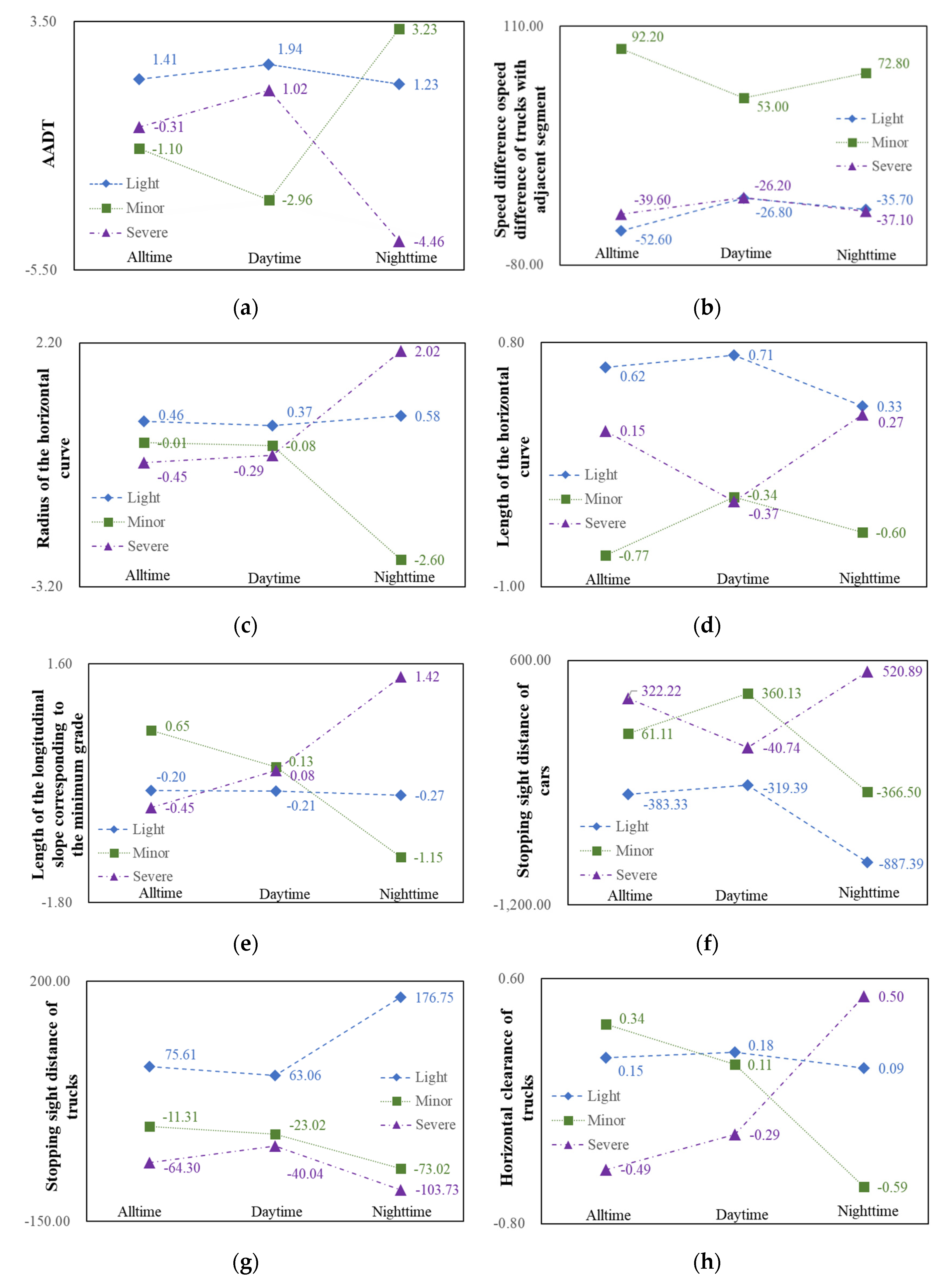
The elasticity effects of the contributing factors for all daytime and nighttime crashes with three injury severities were calculated for comparison. As shown in Figure 1, the elasticity effects of $\Delta V_{O-truck}$ and $S_{truck}$ showed the same trend with different degrees of influence for all of the time windows, indicating no variation over time. Fewer light injury and severe injury crashes will occur with a greater $\Delta V_{O-truck}$. The greater stopping sight distance of trucks contributed to a greater number of crashes with light injury severity.

The elasticity effects of the AADT indicated more light and severe injury crashes during daytime (1.94 and 1.02, respectively), and less severe injury crashes during nighttime (−4.46) with a greater traffic volume. This result was reasonable, as drivers tended to cautiously drive to compensate for the shorter visibility in the evening [62], leading to a lower risk propensity.

Apparently, $R_{present}$ showed different influence trends for daytime and nighttime. Additional severe injury crashes along with fewer minor injury crashes will occur during the night with an increase in $R_{present}$. The proportion of severe-injury crashes rose significantly during nighttime (daytime: −0.29; nighttime: 2.02, in Table 7 and Table 8), indicating that driving on segments with smaller curvature during nighttime made drivers more prone to severe crashes.

In addition, the values of $L_{present}$, $L{s}_{min}$, $S_{car}$, and $H_{truck}$ showed the same trend, with higher positive values of the elasticity effects for severe-injury crashes during nighttime than daytime (nighttime to daytime crashes: 0.27 to −0.37, 1.42 to 0.08, 520.89 to −40.74, and 0.50 to −0.29, respectively), as shown in Figure 1d–f,h. Interestingly, regarding the more negative values, the increase in these factors caused fewer minor-injury crashes during nighttime (−0.60, −1.15, −366.50, and −0.59, respectively). Therefore, the estimated results showed that the influences of several factors indicated injury-severity transferability across the time of day.

7. Conclusions and Future Direction

This study explored the effects of the contributing factors on the crash frequency by injury severity of all, daytime, and nighttime crashes that occurred on freeways. With injury severity outcomes classified as light injury, minor injury, and severe injury, the effects of the explanatory variables affecting the crash frequency were examined in terms of crash, traffic, speed, geometric, and sight characteristics. Regarding the model estimations, the lowest AIC and BIC values (2263.87 and 2379.22, respectively) showed the superiority of the RPMNB model in terms of the goodness-of-fit measure. Additionally, the RPMNB model indicated the highest R² (0.25) and predictive accuracy, along with a significantly positive $\alpha$ parameter. Based on the RPMNB models, several explanatory variables including were observed to exhibit relatively stable effects such as $\Delta V_{O-truck}$ and $S_{truck}$, whereas other variables were found to produce variations including AADT, $R_{present}$, $L_{present}$, $L{s}_{min}$, $S_{car}$, and $S_{car}$.

According to the current findings of this study, several recommendations can be indicated as follows: (1) at nighttime, active light-emitting warning messages, speed limit signs, and other reasonable measures should be set up to prevent drivers from speeding or fatigue; (2) education programs or other measures should be implemented to ensure the safe driving of professional drivers; (3) the lane distribution measures for different vehicle types should be suggested to reduce the interference between cars and trucks; and (4) during the design stage, the alignments of curve-grade sections should be optimized to provide continuous and co-ordinated roadway three-dimensional conditions.

Notably, this study is not free of limitations. The data sample was small and future research can benefit from collecting crash data for longer periods and from more freeways. The remaining dataset should be checked for accuracy in terms of under/over-reporting issues, and more detailed and comprehensive data should be collected. Moreover, more advanced statistical count models can be proposed to account for the unobserved heterogeneity.

References

- World Health Organization. Global Status Report on Road Safety 2018; World Health Organization: Geneva, Switzerland, 2018; ISBN 978-92-4-156568-4. [Google Scholar]
- Traffic Management Bureau of the Ministry of Public Security of the People’s Republic of China. Road Traffic Accident Statistics Annual Report of the People’s Republic of China. 2015. Available online: http://www.stats.gov.cn/tjsj/ndsj/2015/indexch.htm (accessed on 1 July 2020).
- Zhang, X.; Pang, Y.; Cui, M.; Stallones, L.; Xiang, H. Forecasting mortality of road traffic injuries in China using seasonal autoregressive integrated moving average model. Ann. Epidemiol. 2015, 25, 101–106. [Google Scholar] [CrossRef] [PubMed]
- Fei, G.; Li, X.; Sun, Q.; Qian, Y.; Stallones, L.; Xiang, H.; Zhang, X. Effectiveness of implementing the criminal administrative punishment law of drunk driving in China: An interrupted time series analysis, 2004–2017. Accid. Anal. Prev. 2020, 144, 105670. [Google Scholar] [CrossRef] [PubMed]
- Wang, C.; Chen, F.; Zhang, Y.; Wang, S.; Yu, B.; Cheng, J. Temporal stability of factors affecting injury severity in rear-end and non-rear-end crashes: A random parameter approach with heterogeneity in means and variances. Anal. Methods Accid. Res. 2022, 35, 100219. [Google Scholar] [CrossRef]
- Christoforou, Z.; Cohen, S.; Karlaftis, M. Vehicle occupant injury severity on highways: An empirical investigation. Accid. Anal. Prev. 2010, 42, 1606–1620. [Google Scholar] [CrossRef]
- Stamatiadis, N.; Psarianos, B.; Apostoleris, K. Nighttime versus Daytime Horizontal Curve Design Consistency: Issues and Concerns. J. Transp. Eng. Part A Syst. 2020, 146, 04019080. [Google Scholar] [CrossRef]
- National Safety Council. National Safety Council Injury Facts 2020 Edition. National Safety Council. 2020. Available online: https://injuryfacts.nsc.org/motor-vehicle/overview/type-of-crash/ (accessed on 1 July 2020).
- CARE (Community Road Accident Database). Annual Statistical Report 2008. 2008. Available online: https://road-safety.transport.ec.europa.eu/statistics-and-analysis/statistics-and-analysis-archive/statistics-accidents-data_en (accessed on 1 July 2020).
- Fors, C.; Lundkvist, S. Night-time Traffic in Urban Areas: A Literature Review on Road User Aspects. VTI Rep. 650A. Available online: https://www.diva-portal.org/smash/get/diva2:675383/FULLTEXT01.pdf (accessed on 1 July 2020).
- NHTSA (National Highway Traffic Safety Administration). NHTSA Campaign Safe and Sober; NHTSA: Washington, DC, USA, 2019. [Google Scholar]
- Mavridi, I.; Psarianos, B.; Antoniou, C. Investigating the impact of night-time on operating speeds in two-lane rural roads. In Proceedings of the 95th Annual Meeting of the Transportation Research Board, Washington, DC, USA, 10–14 January 2016. [Google Scholar]
- Bella, F.; Calvi, A. Effects of simulated day and night driving on the speed differential in tangent-curve transition: A pilot study using driving simulator. Traffic Inj. Prev. 2013, 14, 413–423. [Google Scholar] [CrossRef]
- Mannering, F.; Bhat, C.R. Analytic methods in accident research: Methodological frontier and future directions. Anal. Methods Accid. Res. 2014, 1, 1–22. [Google Scholar] [CrossRef]
- Mannering, F.; Shankar, V.; Bhat, C. Unobserved heterogeneity and the statistical analysis of highway accident data. Anal. Methods Accid. Res. 2016, 11, 1–16. [Google Scholar] [CrossRef]
- Venkataraman, N.; Ulfarsson, G.; Shankar, V.; Oh, J.; Park, M. Model of relationship between interstate crash occurrence and geometrics: Exploratory insights from random parameter negative binomial approach. Transp. Res. Rec. 2011, 2236, 41–48. [Google Scholar] [CrossRef]
- Anastasopoulos, P.; Mannering, F. A note on modeling vehicle accident frequencies with random-parameters count models. Accid. Anal. Prev. 2009, 41, 153–159. [Google Scholar] [CrossRef]
- Venkataraman, N.; Ulfarsson, G.; Shankar, V. Random parameter models of interstate crash frequencies by severity, number of vehicles involved, collision and location type. Accid. Anal. Prev. 2013, 59, 309–318. [Google Scholar] [CrossRef] [PubMed]
- Aguero-Valverde, J. Full Bayes Poisson gamma, Poisson lognormal, and zero inflated random effects models: Comparing the precision of crash frequency estimates. Accid. Anal. Prev. 2013, 50, 289–297. [Google Scholar] [CrossRef] [PubMed]
- Azimi, G.; Rahimi, A.; Asgari, H.; Jin, X. Injury Severity Analysis for Large Truck-Involved Crashes: Accounting for Heterogeneity. Transp. Res. Rec. 2022, 1, 03611981221091562. [Google Scholar] [CrossRef]
- Barua, S.; El-Basyouny, K.; Islam, M. Multivariate random parameters collision count data models with spatial heterogeneity. Anal. Methods Accid. Res. 2016, 9, 1–15. [Google Scholar] [CrossRef]
- Coruh, E.; Bilgic, A.; Tortum, A. Accident analysis with the random parameters negative binomial panel count data model. Anal. Methods Accid. Res. 2015, 7, 37–49. [Google Scholar] [CrossRef]
- Dong, C.; Clarke, D.; Yan, X.; Khattak, A.; Huang, B. Multivariate random-parameters zero-inflated negative binomial regression model: An application to estimate crash frequencies at intersections. Accid. Anal. Prev. 2014, 70, 320–329. [Google Scholar] [CrossRef] [PubMed]
- Buddhavarapu, P.; Scott, J.; Prozzi, J. Modeling unobserved heterogeneity using finite mixture random parameters for spatially correlated discrete count data. Transp. Res. Part B Methodol. 2016, 91, 492–510. [Google Scholar] [CrossRef]
- Anastasopoulos, P.; Mannering, F.; Shankar, V.; Haddock, J. A study of factors affecting highway accident rates using the random-parameters tobit model. Accid. Anal. Prevention. 2012, 45, 628–633. [Google Scholar] [CrossRef]
- Xie, Y.; Zhao, K.; Huynh, N. Analysis of driver injury severity in rural single-vehicle crashes. Accid. Anal. Prev. 2012, 47, 36–44. [Google Scholar] [CrossRef]
- Behnood, A.; Mannering, F. An empirical assessment of the effects of economic recessions on pedestrian-injury crashes using mixed and latent-class models. Anal. Methods Accid. Res. 2016, 2016. 12, 1–17. [Google Scholar] [CrossRef]
- Malyshkina, N.; Mannering, F.; Tarko, A. Markov switching negative binomial models: An application to vehicle accident frequencies. Accid. Anal. Prev. 2009, 41, 829–838. [Google Scholar] [CrossRef] [PubMed]
- Malyshkina, N.; Mannering, F. Zero-state Markov switching count-data models: An empirical assessment. Accid. Anal. Prev. 2010, 42(1), 122–130. [Google Scholar] [CrossRef] [PubMed]
- Nasri, M.; Aghabayk, K.; Esmaili, A.; Shiwakoti, N. Using ordered and unordered logistic regressions to investigate risk factors associated with pedestrian crash injury severity in Victoria, Australia. J. Saf. Res. 2022, 81, 78–90. [Google Scholar] [CrossRef] [PubMed]
- Yadav, A.; Velaga, N. Alcohol-impaired driving in rural and urban road environments: Effect on speeding behaviour and crash probabilities. Accid. Anal. Prev. 2020, 140, 105512. [Google Scholar] [CrossRef]
- Yadav, A.; Velaga, N. Modelling brake transition time of young alcohol-impaired drivers using hazard-based duration models. Accid. Anal. Prev. 2021, 157, 106169. [Google Scholar] [CrossRef]
- Wei, Z.; Wang, X.; Zhang, D. Truck crash severity in New York city: An investigation of the spatial and the time of day effects. Accid. Anal. Prevention. 2017, 99, 249–261. [Google Scholar]
- Ackaah, W.; Apuseyine, B.; Afukaar, F. Road traffic crashes at night-time: Characteristics and risk factors. Int. J. Inj. Control. Saf. Promotion. 2020, 27, 392–399. [Google Scholar] [CrossRef]
- Malyshkina, N.; Mannering, F. Markov switching multinomial logit model: An application to accident-injury severities. Accid. Anal. Prevention. 2009, 41, 829–838. [Google Scholar] [CrossRef]
- Xiong, Y.; Tobias, J.; Mannering, F. The analysis of vehicle crash injury-severity data: A Markov switching approach with road-segment heterogeneity. Transp. Res. Part B 2014, 67, 109–128. [Google Scholar] [CrossRef]
- Alnawmasi, N.; Mannering, F. A statistical assessment of temporal instability in the factors determining motorcyclist injury severities. Anal. Methods Accid. Research. 2019, 22, 100090. [Google Scholar] [CrossRef]
- Dabbour, E.; Dabbour, O.; Martinez, A. Temporal stability of the factors related to the severity of drivers’ injuries in rear-end collisions. Accid. Anal. Prevention. 2020, 142, 105562. [Google Scholar] [CrossRef] [PubMed]
- Islam, M.; Mannering, F. A temporal analysis of driver-injury severities in crashes involving aggressive and non-aggressive driving. Anal. Methods Accid. Research. 2020, 27, 100128. [Google Scholar] [CrossRef]
- Mannering, F. Temporal instability and the analysis of highway accident data. Accid. Anal. Prevention. 2018, 17, 1–13. [Google Scholar] [CrossRef]
- Tamakloe, R.; Hong, J.; Park, D. A copula-based approach for jointly modeling crash severity and number of vehicles involved in express bus crashes on expressways considering temporal stability of data. Accid. Anal. Prevention. 2020, 146, 105736. [Google Scholar] [CrossRef]
- Wang, C.; Chen, F.; Zhang, Y.; Cheng, J. Spatiotemporal instability analysis of injury severities in truck-involved and non-truck-involved crashes. Anal. Methods Accid. Research. 2022, 34, 100214. [Google Scholar] [CrossRef]
- Yu, M.; Zheng, C.; Ma, C.; Shen, J. The temporal stability of factors affecting driver injury severity in run-off-road crashes: A random parameters ordered probit model with heterogeneity in the means approach. Accid. Anal. Prevention. 2020, 144, 105677. [Google Scholar] [CrossRef]
- Yu, M.; Ma, C.; Shen, J. Temporal stability of driver injury severity in single-vehicle roadway departure crashes: A random thresholds random parameters hierarchical ordered probit approach. Anal. Methods Accid. Research. 2021, 29, 100144. [Google Scholar] [CrossRef]
- Winkelmann, R. Seemingly unrelated negative binomial regression. Oxf. Bull. Econ. Statistics. 2000, 62, 553–560. [Google Scholar] [CrossRef]
- Gouriéroux, C. The Econometrics of Discrete Positive Variables: The Poisson Model. Econometrics of Qualitative Dependent Variables; University Press: New York, NY, USA; Cambridge, UK, 2000. [Google Scholar]
- Berk, R.; MacDonald, J. Overdispersion and Poisson regression. J. Quant. Criminol. 2008, 24, 269–284. [Google Scholar] [CrossRef]
- Chib, S.; Winkelmann, R. Markov chain Monte Carlo analysis of correlated count data. J. Bus. Econ. Statistics. 2001, 19, 428–435. [Google Scholar] [CrossRef]
- El-Basyouny, K.; Barua, S.; Islam, T. Investigation of time and weather effects on crash types using full Bayesian multivariate Poisson lognormal models. Accid. Anal. Prev. 2014, 73, 91–99. [Google Scholar] [CrossRef] [PubMed]
- Aguero-Valverde, J.; Jovanis, P. Bayesian multivariate Poisson lognormal models for crash severity modeling and site ranking. Transp. Res. Record. 2009, 2136, 82–91. [Google Scholar] [CrossRef]
- Winkelmann, R. Econometric Analysis of Count Data; Springer: Berlin/Heidelberg, Germany, 2008. [Google Scholar]
- Spiegelhalter, D.; Best, N.; Carlin, B.P.; Linde, A. Bayesian measures of model complexity and fit. J. R. Stat. Soc. B 2002, 64, 583–639. [Google Scholar] [CrossRef]
- Wang, C.; Chen, F.; Cheng, J.; Bo, W.; Zhang, P.; Hou, M.; Xiao, F. Random-Parameter multivariate negative binomial regression for modeling impacts of contributing factors on the crash frequency by crash types. Discret. Dyn. Nat. Society. 2020, 2020, 6621752. [Google Scholar] [CrossRef]
- Ministry of Transportation of the People’s Republic of China. Specifications for Highway Safety Audit: JTG B05-2015; People’s Communications Press: Beijing, China, 2016. [Google Scholar]
- Ministry of Transport, PRC. Guidelines for Design of Highway Grade-separated Intersections: JTG/T D21-2014; Ministry of Transport, PRC: Beijing, China, 2014.
- Bhowmik, T.; Yasmin, S.; Eluru, N. Do we need multivariate modeling approaches to model crash frequency by crash types? A panel mixed approach to modeling crash frequency by crash types. Anal. Methods Accid. Res. 2019, 24, 100107. [Google Scholar] [CrossRef]
- Solomon, D. Accidents on Main Rural Highways Related to Speed, Driver, and Vehicle; Bureau of Public Roads, U.S. Department of Transportation: Washington, DC, USA, 1964. [Google Scholar]
- Zhong, L.D.; Sun, X.; Chen, Y. The relationship between the speed difference and the accident rate of large and small car on expressway. J. Beijing Univ. Technology. 2007, 33, 185–188. [Google Scholar]
- Korkut, M.; Ishak, S.; Wolshon, B. Freeway truck lane restriction and differential speed limits crash analysis and traffic characteristics. Transp. Res. Record 2010, 2194, 11–20. [Google Scholar] [CrossRef]
- Huang, H.; Chin, H.; Haque, M. Severity of driver injury and vehicle damage in traffic crashes at intersections: A Bayesian hierarchical analysis. Accid. Anal. Prevention. 2008, 40, 45–54. [Google Scholar] [CrossRef]
- Sarhan, M.; Hassan, Y. Three-Dimensional, Probabilistic Highway Design: Sight Distance Application. Transp. Res. Rec. J. Transp. Res. Board 2008, 2060, 10–18. [Google Scholar] [CrossRef]
- Fountas, G.; Fonzone, A.; Gharavi, N.; Rye, T. The joint effect of weather and lighting conditions on injury severities of single-vehicle accidents. Anal. Methods Accid. Research. 2020, 27, 100124. [Google Scholar] [CrossRef]