Article

Studying the Effect of Blue-Green Infrastructure on Microclimate and Human Thermal Comfort in Melbourne’s Central Business District

1
College of Engineering and Science, Victoria University, P.O. Box 14428, Melbourne, VIC 8001, Australia
2
Institute for Sustainable Industries and Liveable Cities, Victoria University, P.O. Box 14428, Melbourne, VIC 8001, Australia
3
Department of Land Surveying and Geo-Informatics, The Hong Kong Polytechnic University, Hong Kong, China
4
College of Engineering, Information Technology and Environment, Charles Darwin University, Ellengowan Drive, Brinkin, NT 0810, Australia
*
Author to whom correspondence should be addressed.
Sustainability 2022, 14(15), 9057; https://doi.org/10.3390/su14159057
Submission received: 17 June 2022 / Revised: 20 July 2022 / Accepted: 20 July 2022 / Published: 24 July 2022
(This article belongs to the Topic Urban Mitigation and Adaptation to Climate Change)

Abstract

:
Blue-green infrastructure (BGI) is defined as a strategically planned network of natural and semi-natural areas with other environmental features designed and managed to deliver a wide range of ecosystem services, which include microclimate regulation and enhanced human thermal comfort. While green infrastructure is widely known to be capable of mitigating the adverse effects of urban heat island, the effect of blue infrastructure to regulate thermal comfort is still poorly understood. This study investigates several blue-green-infrastructure (BGI) scenarios in the central business district (CBD) of Melbourne, Australia to assess their effects on microclimate and human thermal comfort. Three-dimensional microclimatic modelling software, ENVI-met, was used to simulate the microclimate and human thermal comfort. Physiological equivalent temperature (PET) was used to quantify the level of thermal comfort in selected research areas. Ten different scenarios were simulated, which included those based on green roofs, green walls, trees, ponds and fountains. The simulations suggest that green roofs and green walls in the high-rise building environment have a small temperature reduction in its surrounding area by up to 0.47 °C and 0.27 °C, respectively, and there is no noticeable improvement in the level of thermal perception. The tree-based scenarios decrease temperature by up to 0.93 °C and improve the thermal perception from hot to warm. Scenarios based on water bodies and fountains decrease the temperature by up to 0.51 °C and 1.48 °C, respectively, yet they cannot improve the thermal perception of the area. A deeper water body has a better microclimate improvement as compared to a shallow one. The temperature reduction in the fountain scenario tends to be local and the effect could only be felt within a certain radius from the fountain.

1. Introduction

Although urban areas currently cover less than 5% of the world’s land surface [1], more than half of the world’s population lives in cities and this is likely to increase to 70% by 2025. With this rapid growth in cities, the urban environment is vulnerable to degradation. Through substantial conversion of natural green areas such as forest and agriculture to urban areas, many cities are experiencing the urban-heat-island (UHI) phenomenon, which makes urban temperatures higher than that of surrounding areas. Higher temperature in urban areas generates uncomfortable and precarious effects on essential aspects of human lives, such as human health, water consumption, energy use, and air quality [2,3,4,5,6]. To counter these effects, various mitigation measures have been introduced, which include the implementation of blue-green infrastructure. Green infrastructure (GI) is an interconnected network of green space that conserves natural ecosystem values and functions and provides associated benefits to human populations [7]. These include parks, gardens, woodlands, green corridors, street trees, green roofs and green walls. GI is capable of regulating microclimate through evapotranspiration and shading of the surfaces through its canopy, and positively affects environmental thermal comfort [8]. Microclimate is defined as the climate in a local region that differs from that in the surrounding regions [9]. Due to this capability, GI is often mentioned as a key strategy for UHI mitigation as well as climate-change adaptation. Currently, the concept of GI has been emphasized in Melbourne as a part of a broader set of ESD (environmentally sustainable design) principles. This is expected to help the city to maintain its status as one of the most livable cities in the world. Although studies on the benefits of GI for mitigating the adverse impacts of UHI have been widely conducted, including a few in Melbourne [10,11], it is observed that some types of GI are less investigated than the others. Green walls, for example, were only researched by 4.3% studies reviewed by Balany et al. [12]. As the number of available studies on green walls is few, it is insufficient to provide a concrete conclusion regarding their ability to improve microclimate and human thermal comfort. Furthermore, while several types of GI have been proven to mitigate the adverse effects of UHI, the capability of blue infrastructure (BI) to mitigate the negative effect of UHI is not yet well-understood. Research on BI has not been explored as much as that on GI, not to mention those that are located in Melbourne. GI and BI together are often referred to as blue-green infrastructure (BGI). As the benefit of BGI varies by location, they should be investigated locally. Therefore, to assess the capability of BGI to mitigate the UHI in Melbourne, this study quantitatively evaluates the cooling capacity of GI and BI strategies through the use of a numerical simulation model ENVI-met. In this study, the best possible GI and BI strategies to maintain enhanced microclimate and improve thermal comfort were identified. The rest of the paper is organized as follows. A literature review is briefly covered in Section 2. The methodology used in this study will be presented in Section 3, while Section 4 presents the results and discussion. Finally, conclusions from this study are drawn in Section 5.

2. Literature Review

GI and its cooling effect have been extensively studied around the world in different climatic regions [12], such as arid and semi-arid [13,14,15], temperate [16,17], and tropical [18,19]. Different types and locations of GI were investigated including green roofs [14], urban parks [20,21,22], street vegetation [23], and residential vegetation [24,25]. In regulating urban microclimate and thermal comfort, the benefit of GI varies by location, the size of the areas [18], and species [26]. The temperature reduction depends heavily on canopy covers [27,28] and the health status of vegetation, which is indicated by the chlorophyll content [29,30].
BGI commonly includes green spaces (such as trees, parks, fields and forests) and natural or man-made water elements (such as rivers, fountains, ponds, canals, and wetlands). BGI is widely utilized to manage stormwater and reduce flood risk. In addition, BGI can mitigate the impact of climate change such as heatwaves, extreme storms, and drought; enhance wild life and biodiversity; improve mental health and wellbeing and create attractive landscapes [31]. BGI are not limited to the urban area and may exist at different geographic levels (e.g., rural, catchment, and regional areas) and jurisdictional boundaries and, thus, this should be taken into consideration in its planning. The benefit of BGI can only be fully realized through an interconnected network of its constituent elements; hence, connectivity is a crucial concept in BGI [32]. Water bodies contribute to cooling down their surrounding area through two mechanisms: evaporation and convection [33]. When evaporation occurs, the energy is removed from the water bodies and eventually the temperature of the bodies reduces, resulting in evaporative cooling. This reduces water temperatures and will affect sensible heat fluxes. If a water surface is cooler than air, the sensible heat flux will be directed toward the water and, as a result, this process can cool the air [34]. Conversely, warmer water can increase the surrounding air temperature. The contribution of water bodies in improving outdoor thermal comfort may be significant and should not be neglected, since evaporation of 2000 m3 of water can lower the temperature by 1K [35]. In addition, water bodies showed the lowest temperature among other urban materials, especially during the summer, and become the warmest during the winter [36]. Some research regarding the cooling capacity of water has been conducted in several parts of the world (the Netherlands, Israel, China, Hungary, and South Korea) with different types of BI such as wetland [37], water bodies (sea, lake, canal) [34,36,38], streams and rivers [39], ponds [40], fountains [41], and water spray systems [42]. Coutts et al. [43] compiled studies of the cooling effect of water bodies on the climate of urban areas. The studies suggested temperature reduction in adjacent and downwind of water bodies by 1–2 °C, especially during the day. These temperature reductions were attributed to evaporation or the downwind cooling effect of the water bodies. Fountains were also found to have a cooling effect in the leeward area [41], with the temperature reduction being 1–4 °C. However, the latter study found that some small urban water bodies (such as canals, ditches and ponds) in the Netherlands only have a very small cooling effect on their surrounding area and, thus, they may be neglected in climate-responsive design practices [34]. Some factors effecting the cooling capability of water bodies included geometry, proportion of vegetation and impervious surfaces [35]. In Australia, research on the cooling effect of BI is still lacking and is also not comprehensive. A study by Broadbent [44] found that increasing irrigation on a grassland area in Lake Mason in Adelaide has a cooling effect of up to 1.75 °C at 13:00 and a small warming effect at night (<0.75 °C). The planning process in BGI projects require interdisciplinary cooperation, as it combines both greening and water aspects [45].
The microclimate of an area is controlled by complex environmental variables such as temperature, solar radiation, humidity and wind. Characteristics of microclimates are also heavily influenced by structures in the area, such as buildings, vegetation, construction material used, etc., and, hence, microclimate is also frequently referred to as the “climate near the ground” [46]. Thermal comfort is defined by the British standard BS EN ISO 7730/ISO 7730 1994 and also ASHRAE 1989 as being “that condition of mind which expresses satisfaction with the thermal environment”. The factors influencing thermal comfort can be environmental as well as personal aspects, although some non-thermal environmental factors such as ambient light and noise may affect people’s thermal sensation [47,48]. Environmental factors include air temperature, radiant temperature, humidity and wind speed, whereas personal factors consist of metabolic rate/activity and clothing, which influences the heat and mass transfer rates between the human body and the environment. In addition, population characteristics, previous accommodation, personal preference and mood also may influence the level of thermal sensation. Thermal comfort in various climates has been intensively studied [17,18,49,50,51,52,53,54]. To assess the level of thermal comfort/discomfort, some thermal comfort indices are used. More than 100 indices have been developed for both indoor and outdoor studies [55]. PET, for example, is one of the most widely used indexes in thermal-comfort studies [49,50,53,56]. PET, which was developed for outdoor settings, is based on the Munich Energy-balance Model for Individuals (MEMI) [57]. Some limitations of PET regarding air humidity and clothing factor, particularly in hot and humid regions, are addressed through modified physiologically equivalent temperature (mPET) [52]. The mPET, then, has proven to perform well in Freiburg Germany and adapt better to the hot and humid region of Taiwan [58]. However, instead of personal thermal comfort, these thermal comfort models predict the average response of a large population, which is less accurate at representing individual perception.
Melbourne (37°48′ S 144°57′ E) is the capital of the state of Victoria. Based on the Koppen climate classification, Melbourne has a temperate oceanic climate (cfb), with warm to hot summers and mild winters. Contrary to most northern hemisphere cities, summer in Melbourne usually starts in December while winter begins in June. Mean annual temperature is 16.2 °C while the highest temperature ever recorded was 46.4 °C and the lowest was −2.8 °C. Rainfall average is 601 mm per annum, occurring mainly in summer. Melbourne has been subjected to rapid population growth in the recent past, a process which has led to changes in land use such as increased urban and built-up areas. The city recorded the largest and fastest population growth among all of Australia’s capital cities during 2016–2017. The research area, Melbourne’s CBD, has become the most densely populated area in Australia with a density of 22,400 people per sq km as of June 2020 (www.abs.gov.au, accessed on 14 October 2020). The area, characterised by high-rise and high-density buildings, has warmer temperatures than any other area in the city [59]. Due to restricted land availability and the efficiency of transport infrastructure, Melbourne promotes a more compact settlement, especially in the city-centre area. However, this strategy potentially intensifies the UHI. To mitigate the adverse effect of UHI and maintain its liveability, the city has incorporated GI in its planning. A better and comprehensive assessment on how blue-green infrastructure contributes to improving thermal comfort is important for urban planning to enhance the liveability and sustainability of the city.

3. Materials and Methods

Melbourne CBD was selected to be assessed in terms of thermal comfort in the oceanic temperate climate of Melbourne. Figure 1 shows the method used in this study, which is comprised of two main parts: (1) digitizing and input data, and (2) simulation. The calibrated ENVI-met was used to simulate blue-green infrastructure scenarios in the research area. ENVI-met simulated the microclimates’ data such as air temperature (Ta), relative humidity (RH), mean radiant temperature (MRT) and wind speed (Ws). These data were used by Bio-met (a post-processor tool of ENVI-met) to calculate PET, which indicates thermal comfort.

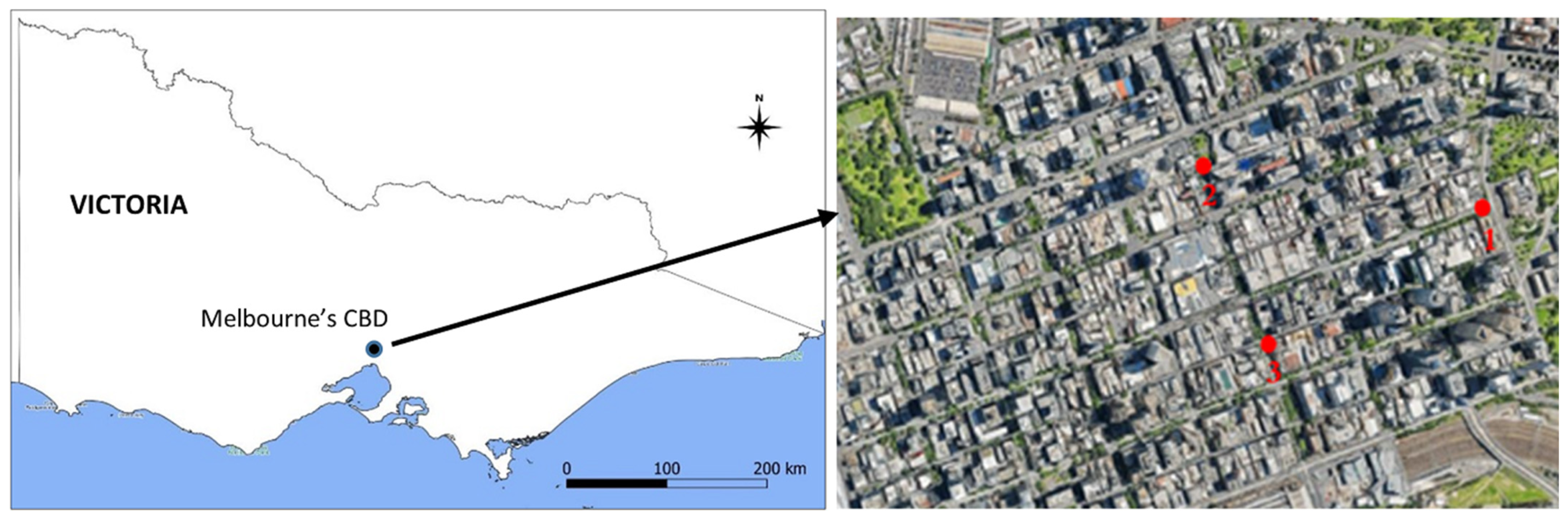
3.1. Data Collection

Field measurements and data collection from the Bureau of Meteorology (BoM), Australia were conducted in this study. Field measurement was designed to collect microclimate data for model validation. Field measurements in Melbourne CBD were performed in an area around the Parliament House, Chinatown Melbourne and the Melbourne Town Hall. These areas are marked as 1, 2, and 3 in Figure 2, representing the Parliament House, Chinatown and the Town Hall, respectively. The data was collected for few days during January of 2020. January was selected as the time to conduct the field measurements as the highest air temperatures were recorded in summer during the past year. HOBO MX2301A logger was used for monitoring the Ta and RH. The instrument was set up in a safe point in each area and secured against wind gusts in order to assess their climate. The data logger was pre-modified to record the information continuously every 10 min. In addition, daily microclimate data from Olympic Park station (www.bom.gov.au, accessed on 1 February 2020) were retrieved, including Ta, RH, wind speed and direction. The Olympic Park station is the nearest weather observation station to Melbourne CBD, located approximately 2.5 km southeast of the CBD. These data were used as the input for model initialization, while the field measurement data were used to validate the model.

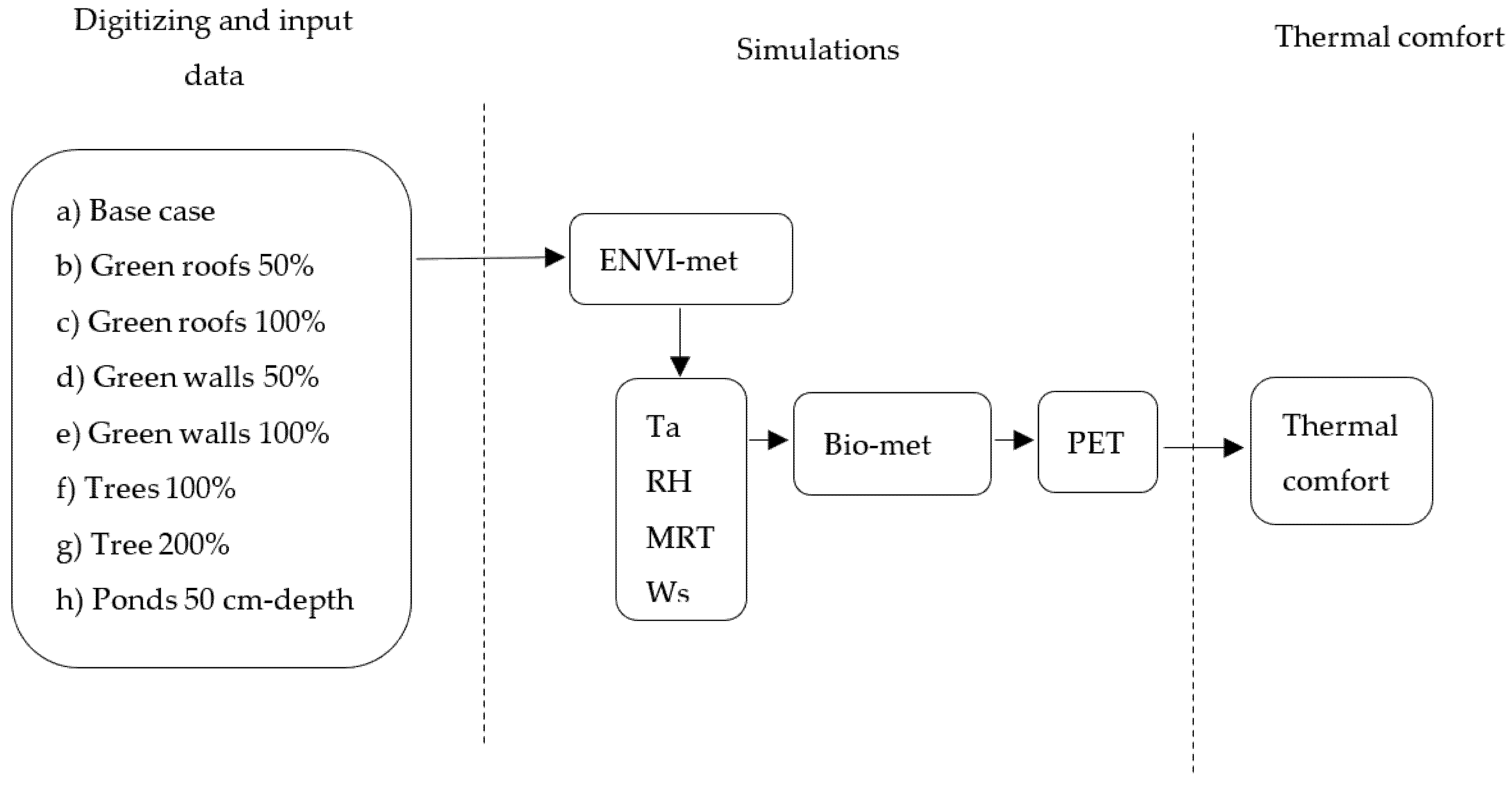
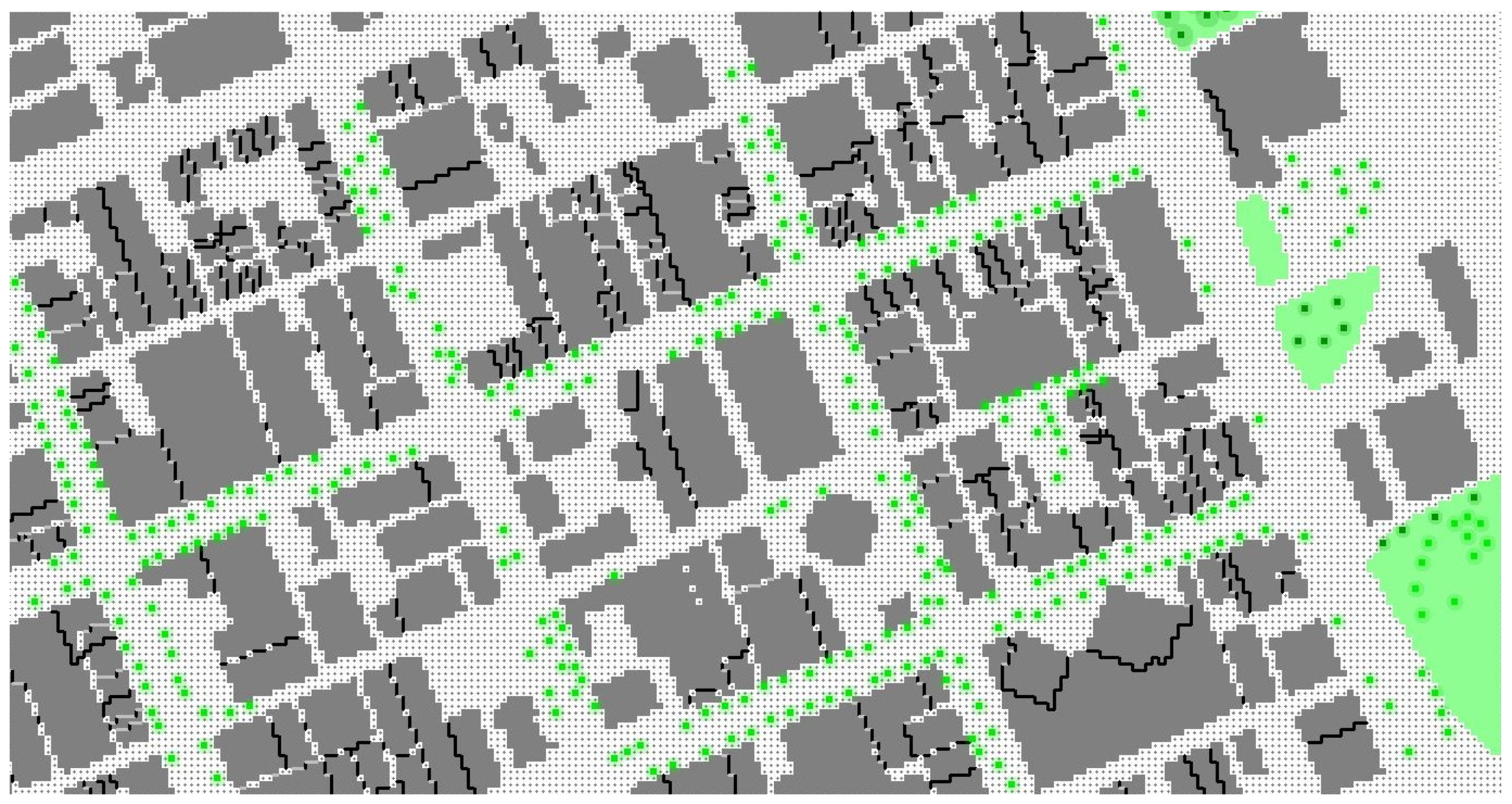
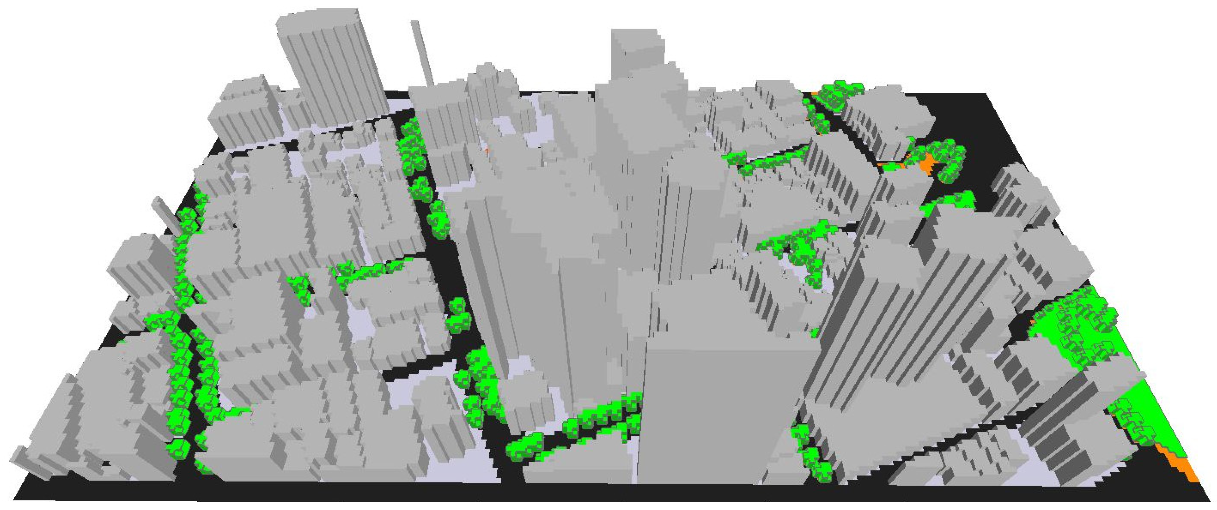
3.2. Model Configuration

ENVI-met 4.4 [60] combines calculation of fluid dynamic parameters such as wind flow or turbulence with the thermodynamic processes taking place on the ground surface, walls, roofs and vegetation. An input file and the main configuration parameters are required for the simulation. The input file is needed to build spatial properties of the research area such as geographical location, building characteristics, surface and vegetation with resolution of 0.5 to 10 m in space and 10 s in time. Area to be modelled is digitized on rectangular grids with maximum grids of 250 × 250 cells.
Melbourne CBD area was set at 234 × 128 × 40 cells with a grid cell size of 4 m. In addition, 10 nesting grids were applied in the model area. It is recommended for large modelling domain that nesting grid should be set to a minimum of 3 [61]. Most of the available 3D models do not work reliably on the grids close to the border. Hence, a nesting grid aims to reduce errors at the boundary, thus making the model reliable and stable. In digitizing the model area, a vector-based editor MONDE was applied. This editor enables the creation of layers of GIS geometry, such as nodes, lines and polygons, to represent buildings, roads and vegetation. MONDE allows importing GIS shape files and Open Street Map (OSM) layers to use them as input for the INX files. OSM is a 2-dimensional free online GIS map that also supports data gathered by individual contribution from volunteers. Like GIS, features in OSM carry attributes (for instance, buildings have a height attribute). However, as data in OSM is not always complete (for example, building heights might be missing), the assignment of the attribute then has to be carried out by the user, using either other sources or field measurement data. In this study, some missing building heights were assigned using data from ArcGis web map and open data available from the City of Melbourne. Given that there are many high-rise buildings in the research area, the telescoping factor was activated at 30%, which allows the vertical grid size to expand with the height of buildings. Roughness length (Z0) was set to 2.0, since the study area is in an urban area with high-rise buildings [62]. In ENVI-met, the maximum possible value of Z0 should be half the size of the lowest grid cell. Once the Z0 value is too high for a chosen vertical resolution, ENVI-met will automatically reduce the value to the maximum possible value. The material of the buildings were mainly concrete and dark-coloured façade. Therefore, the albedo of the buildings was adjusted to a low value, namely, 0.2 and 0.3 for walls and roofs, respectively. The ground surface materials were mainly asphalt and concrete pavements and ENVI-met’s default properties for those materials were adopted. Some simple and 3D plants such as plane trees (Platanus × Acerifolia), palm trees, hosta and grass were selected to represent vegetation in the study area. These types of plants were chosen as they are the most common types that are growing in the area. ENVI-met allows the user to develop a personal database of plants with attributes such as personalized height, leaf area density (LAD) and root area density (RAD). In this study, the plane trees were set to a height of 13 m. The types, amount and location of vegetation were determined based on field observation as well as data from Opentrees website. The modification of trees was performed using the ALBERO tool in ENVI-met. The simulation configuration is presented in Table 1, while two- and three-dimensional views of the research area can be seen in Figure 3 and Figure 4, respectively.
Full forcing mode was applied as it is considered to provide higher simulation accuracy and more realistic results. Full forcing mode provides the possibility of user-defined diurnal variations in atmospheric boundary conditions (forcing), allowing the creation of user-specific weather scenarios. The parameters that can be forced include radiation, wind speed and direction, air temperature, specific humidity and background concentration of particles/gases. In addition, ENVI-met requires initialization time to allow the model to follow atmosphere phenomena [63]. Initialization time also provides enough time for the urban material to heat up. It is recommended that the simulation starts before sunrise and has longer than 6 h running time [19]. This study aims to examine different BGI performances to mitigate human thermal stress, which is especially an issue during summer. Hence, undertaking the simulations during a typical hot summer day in Melbourne was considered appropriate to represent microclimate and thermal comfort conditions during summer. The simulation time was set up at 06:00 am with a time period of 48 h, starting at 06:00 am on 12 January and ending at 06:00 am on 14 January. Two days of simulation was chosen, as this was considered sufficient to generate valid outputs to represent microclimate and thermal comfort conditions of the study area [64]. The first 24 h were used as initialization time and the last 24 h were used for data analysis. Deduction and data analysis were carried out using Leonardo tool. The tool, which is part of ENVI-met, can visualize the outcome both in 2D and 3D forms.
Thermal comfort was calculated using Biomet, which is a post-processing tool in ENVI-met. The tool directly interacts with ENVI-met output (Ta, RH, Ws and MRT) to generate thermal comfort indices. These aforementioned parameters are primary factors that must be addressed when defining thermal comfort. In addition, some personal human parameters need to be set, such as age, gender, weight, height, clothing insulation and metabolic rate. In this study, physiological equivalent temperature (PET) [57] index was used to measure the level of thermal comfort. PET classifies the level of heat stress into nine categories starting from cold (<4 °C) to very hot (>41 °C). A value between 18 °C and 23 °C is considered as comfortable. The numerical threshold for PET index is given in Table 2. PET index was calculated for a 35 year-old man, 1.75 m tall, 75 kg in weight with a metabolic rate of 164.49 W/m2 and clothing insulation of 0.9 m2 K/W.

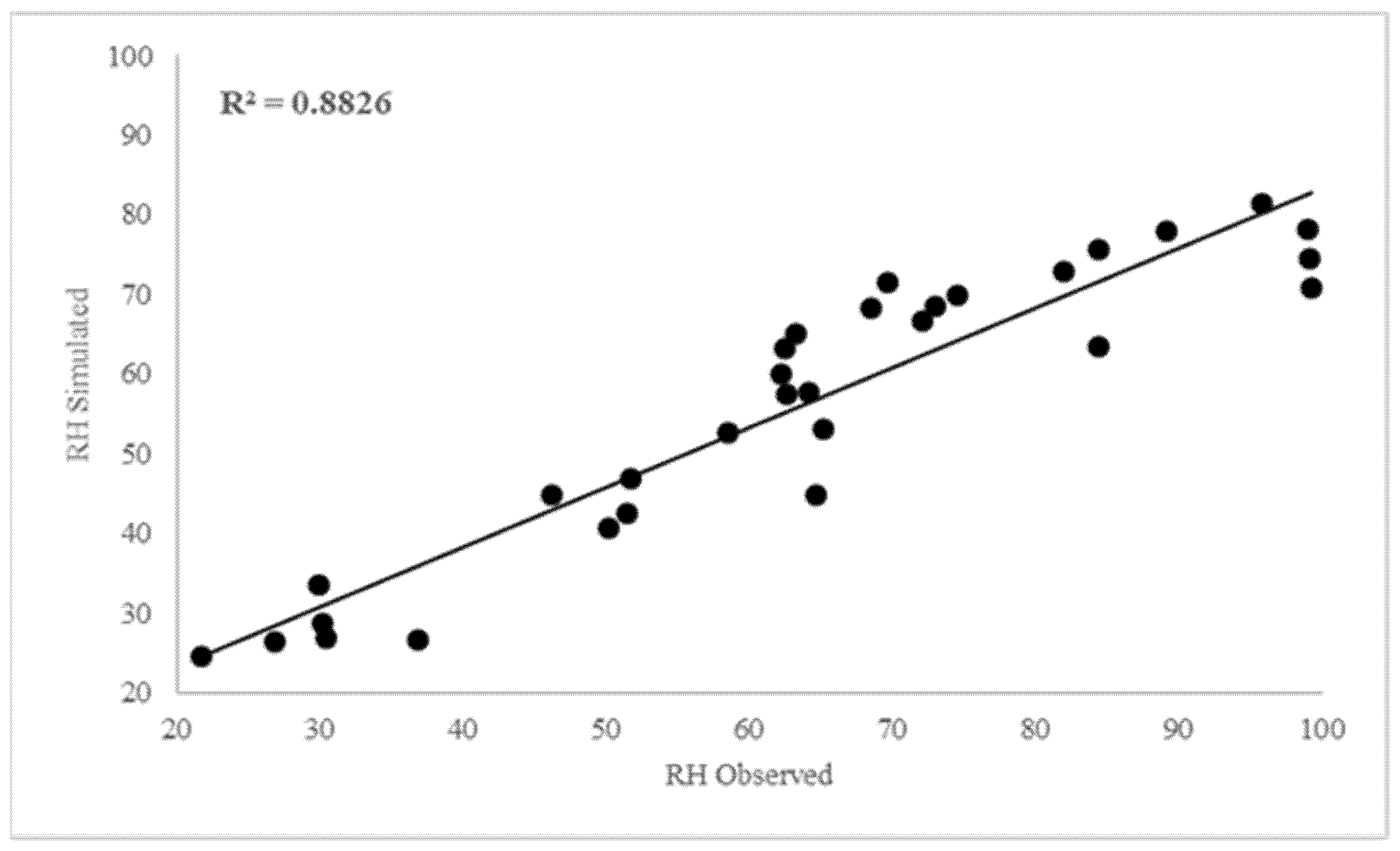
3.3. Model Validation
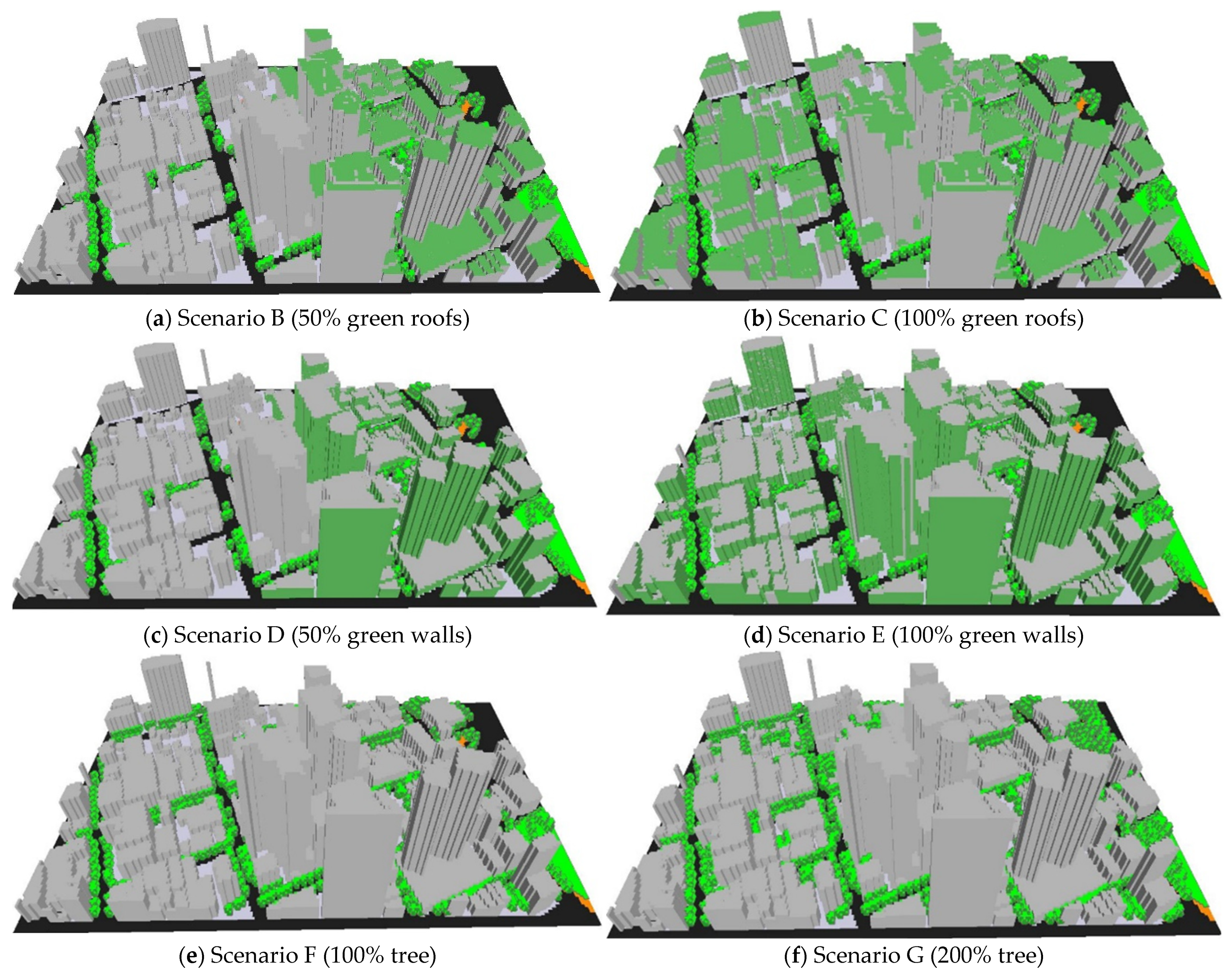
The reliability of simulation results depends on the input data and initial boundary condition. In this study, the accuracy of ENVI-met model was assessed by comparing the series of field-measurement data and the corresponding simulated results. As mentioned earlier, three locations within Melbourne’s CBD were selected for the field measurements, which was carried out on 5 January 2020. Parameters Ta and RH were used in validation of the research area. The hourly value of Ta and RH were examined in the period 06:00–17:00. To verify the model validation result, statistical evaluation of model performance was undertaken using the coefficient of determination (R2), root mean square error (RMSE) and Willmott’s index of agreement. R2 describes the proportion of the variance in measured data explained by the model and was analysed by using scatter plot distribution. R2 values greater than 0.5 were considered acceptable [65]. Root mean square error (RMSE) provides description of the average difference between the observed and simulated values. The RMSE is always non-negative and a value of 0 would indicate a perfect fit to the data, which is almost never achieved in practice. Meanwhile, Willmott index of agreement [66] represents the ratio of the mean square error and potential error. The index value varies between 0 (no agreement) and 1 (perfect fit). Table 3 shows the values of these model evaluation statistics, namely, R2, RMSE and Willmott’s index of agreement. From the table, it can be seen that both Ta and RH are well-predicted with R2 = 0.927, d = 0.948 and R2 = 0.883, d = 0.922, respectively. RMSE of RH is slightly higher than the RH values commonly reported in literature (2.04–10.20%) [67]. Despite this small deficiency, based on R2 and d values, it can be concluded that the model has a strong correlation with observed values and can be considered to adequately represent the actual situation. Regression analysis between the simulated and observed values of Ta and RH are presented in Figure 5 and Figure 6, respectively.

3.4. Case Studies

For evaluating the effect of BGI on microclimate and human thermal comfort, ten scenarios of blue-green infrastructure were developed as follows.
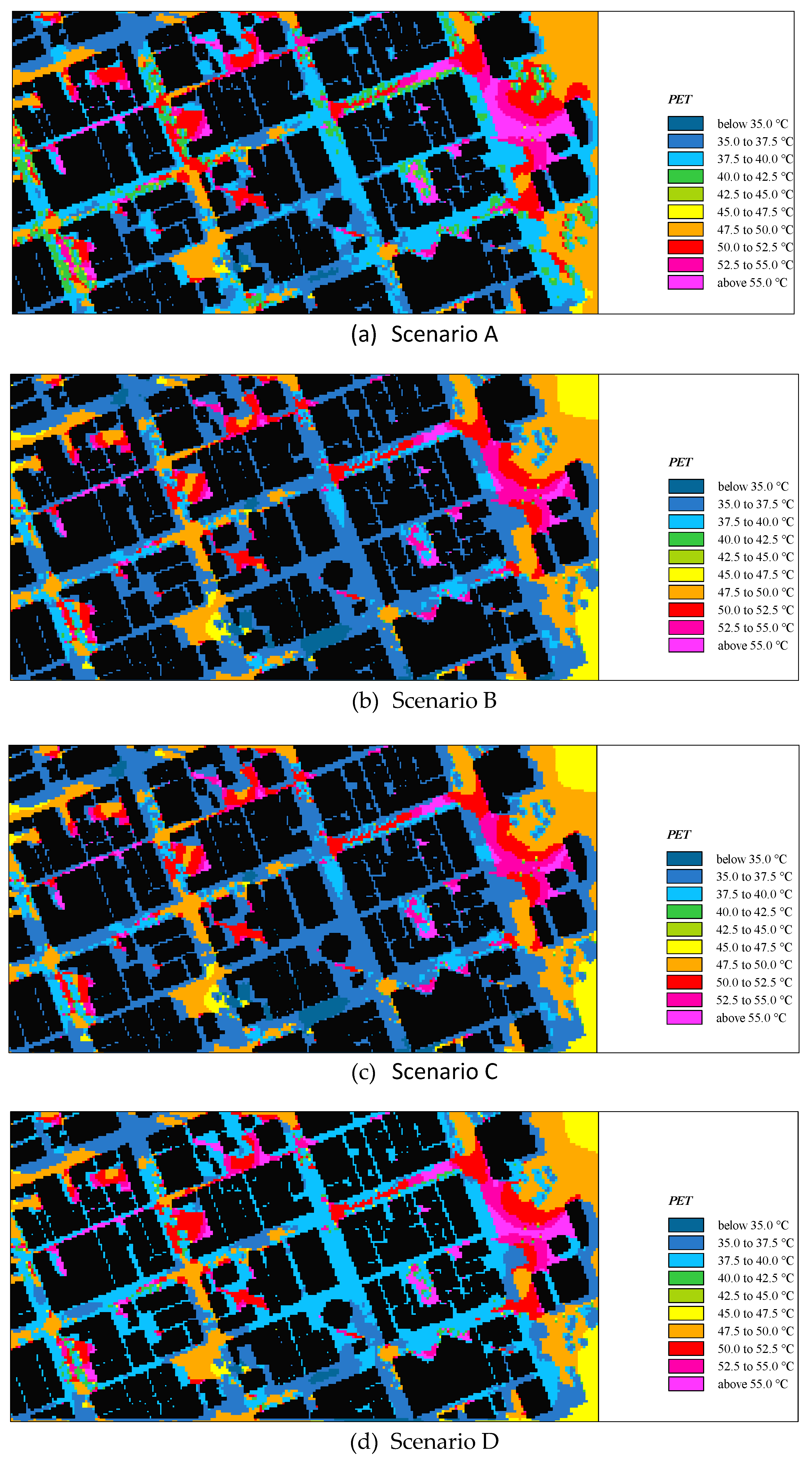
  • Scenario A: the base case, i.e., the current CBD area, including high-rise buildings, concrete pavements and asphalt surfaces, grass and trees.
  • Scenario B: Scenario A with addition of 50% green roofs in the eastern part of the research area.
  • Scenario C: Scenario A with addition of 100% green roofs in the research area.
  • Scenario D Scenario A with addition of 50% green walls in the eastern part of the research area.
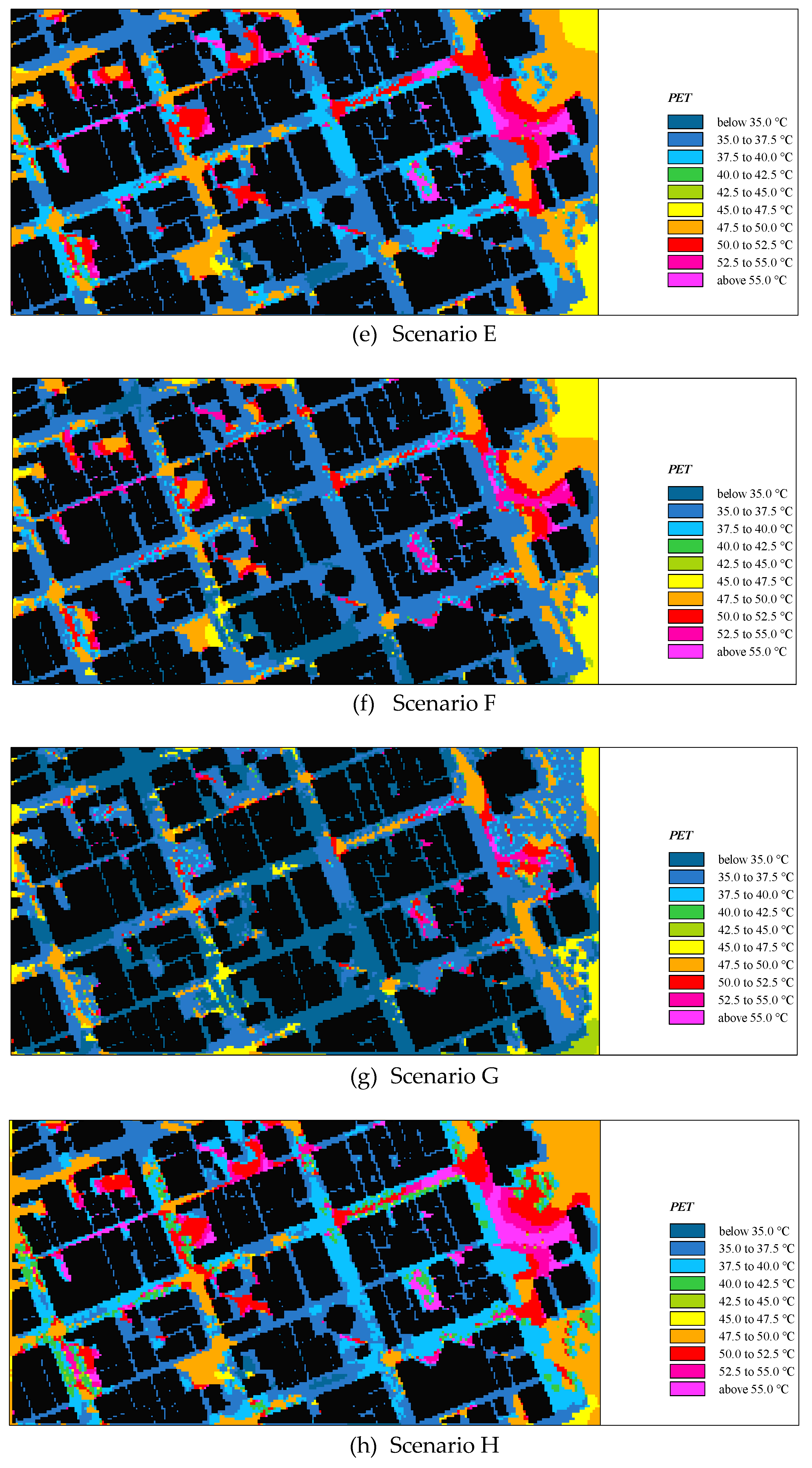
  • Scenario E: Scenario A with addition of 100% green walls in the research area.
  • Scenario F: Scenario A with addition of 100% trees (i.e., double of the existing condition).
  • Scenario G: Scenario A with addition of 200% trees (i.e., triple of the existing condition).
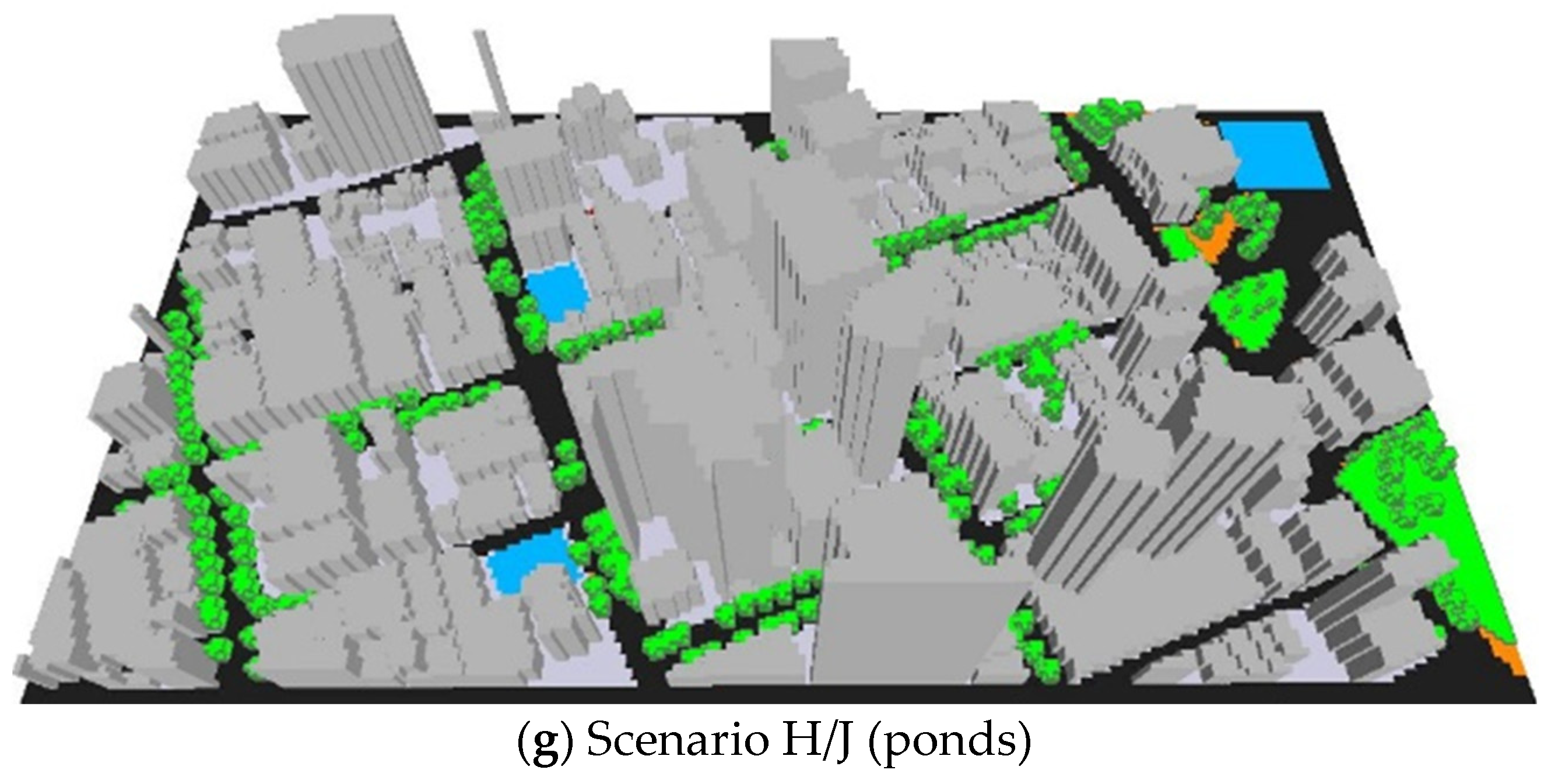
  • Scenario H: Scenario A with addition of 3 ponds, 50 cm in depth, randomly placed in the research area.
  • Scenario I: Scenario A with addition of 3 ponds, 100 cm in depth, randomly placed in the research area.
  • Scenario J: Scenario A with addition of 13 fountains, 4 m in height, randomly placed in the research area.
The layout of Scenario A (base case) and B–J can be seen in Figure 4 and Figure 7, respectively. Greening scenarios were designed using funkia (hosta) plantation with height of 60 cm on the green roofs and 30 cm on the green walls. All the tree scenarios used plane trees with height of 13 m. The default area density (LAD) setting in ENVI-met was used. For the BI scenario, the ponds were placed randomly in the model area where there were spaces available. Water bodies in ENVI-met are represented as a special type of soil. In addition to ponds, another BI scenario (Scenario J) placed 13 fountains of 4 m height in the model area (please see Figure 8 for location of the fountains). All the main parameters have been left unchanged in order to evaluate only the effect of BGI on the urban microclimate and thermal comfort.

4. Results and Discussion

For each of the scenarios of blue and green infrastructure, 28 points were evenly distributed in the model area, from where the results were extracted (Figure 9). Temperature at the points at pedestrian level (1.5 m) were extracted at 15:00 and were plotted as box and whisker graphs (which indicate the minimum and maximum values as well as the upper and lower quartile of the temperature values).

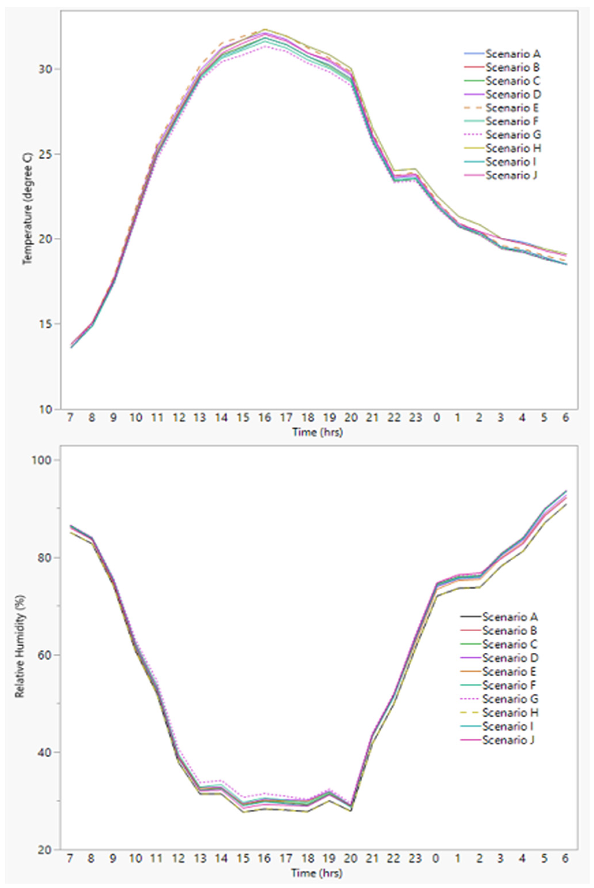
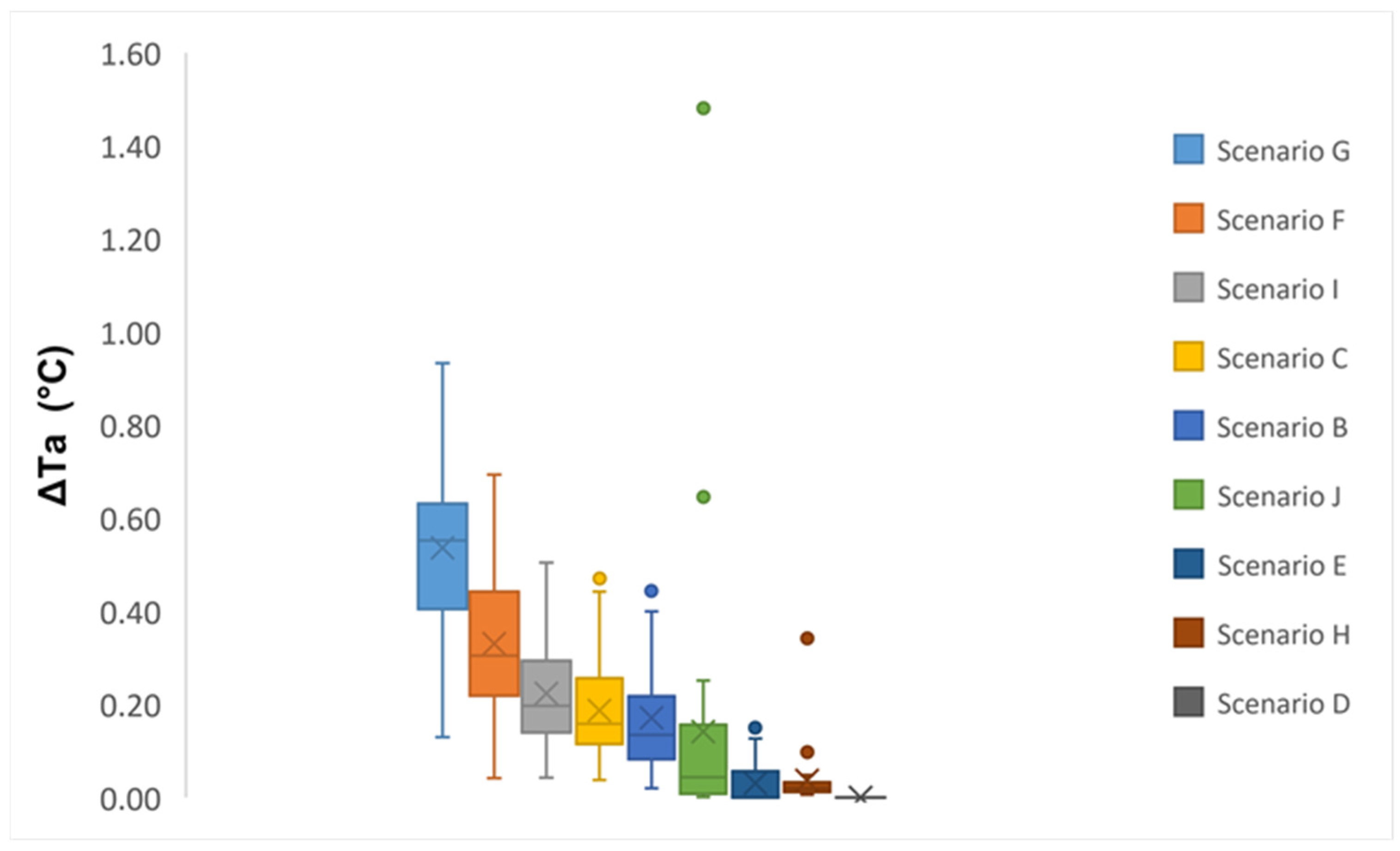
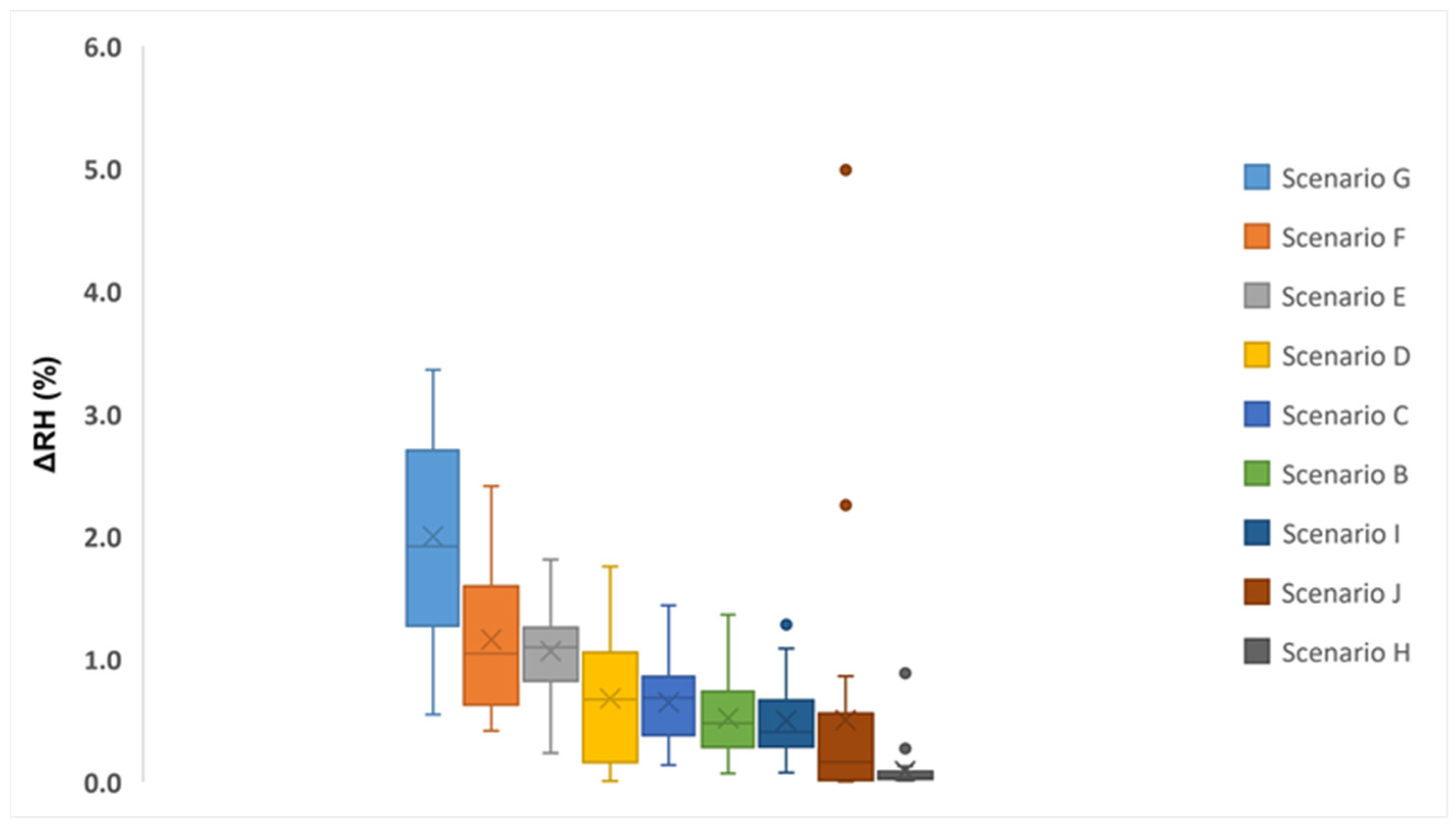
4.1. Air Temperature and Relative Humidity

The relationship between Ta and RH is inversely proportional to each other, i.e., as Ta increases, the RH values decrease. To know the variation in Ta and RH at pedestrian level, one point (point 19) was taken as an example. Hourly profiles of Ta and RH at point 19 are presented in Figure 10 (starting from 07:00 on 13 January to 06:00 on 14 January). All the scenarios have a similar pattern of Ta and RH. Between 07:00 and 16:00, the location (represented by point 19) experienced a rise in temperature that peaked at 16:00, while RH values reached their minimum at that time. At these times, low evaporation and solar radiation absorption also occurred. As the day progressed, Ta values started to decrease and the RH values increased.
Based on ENVI-met simulation results, daytime temperature for Scenarios B–J showed a maximum drop when compared to Scenario A (base case) values during the time range of 12:00–19:00. The maximum temperature reduction at most of the points was recorded at 15:00 and 16:00. Comparing the results between Scenario A and Scenarios B and C (green roofs) showed a low temperature reduction. This result is in-line with studies by Ng et al. and Jamei et al. [11,18], which reported a very low temperature reduction due to the implementation of green roofs. On the contrary, there are other studies which reported a moderate-to-significant temperature reduction caused by the application of green roofs [68,69,70]. In this study, the maximum temperature reduction at 15:00 was recorded as 0.47 °C in Scenario C. This number, however, is quite small considering that all buildings in the area were covered with green roof. The majority of buildings’ height in the research area range between 15–60 m, with some of them being more than 100 m. Green roofs installed on the top of high-rise buildings most likely will not contribute to Ta reduction at pedestrian level (1.5 m). Similar to green roofs, the application of green walls (Scenarios D and E) in Melbourne’s CBD also gave a very small temperature reduction. Although a study reported a remarkable reduction in Ta values (1.86 °C) due to the application of green walls in a city centre of Sri Lanka [68], this was not observed in this study for Melbourne’s CBD. The maximum reduction in Ta at 15:00 recorded was only 0.27 °C in Scenario E (all covered by green walls). Based on these results, it, then, can be concluded that the application of green walls would be less effective in reducing Ta at pedestrian level in Melbourne’s CBD. Covering all the buildings with green walls is considered difficult to achieve or even impractical and, moreover, the reduction in Ta is too small. Although there is no noticeable reduction in Ta, green walls reduced the façade temperature of the buildings at midday. Figure 11 shows the temperature reduction in buildings’ façade at 15:00 (Scenario E), which ranged between 6–10 °C. This result is supported by past studies, where the application of green walls reduced the external wall temperature of buildings during summer by values of between 1.7–16 °C [71]. Some factors influencing the performance of green façades include, type of plants, properties of the layers and shading effect. From the simulation results, it can be seen that the temperature reduction was higher at exposed parts of the buildings than the shadowed parts. Green walls act as a barrier by blocking solar radiation and preventing heat from entering inside the buildings during those hot days. A wall’s surface temperature is directly related to heat loss through the building walls. The higher the wall’s surface temperature, the higher the heat loss through the walls, which potentially increases temperature inside building. As a green wall controls the heat transfer, it, then, can be identified as a passive technique for energy saving in the building [71]. By applying green walls, energy for cooling buildings can be reduced by up to 32 percent [72]. The tree scenarios (of F and G) gave the biggest temperature reduction among the greening scenarios. Scenarios F and G contributed to the maximum air temperature reduction by 0.69 °C and 0.93 °C, respectively. The average value of reduction is 0.3 °C for Scenario F and 0.5 °C for Scenario G, which were higher than the maximum value of Ta reduction from the green roof and green wall scenarios. Tree foliage provides protection from solar radiation and, at the same time, releases water vapour that can reduce surrounding Ta. This result reinforces the outcomes from previous research, which found that trees reduced the temperature by up to 1 °C and more [18,61,68,73,74,75] or less than 1 °C [11,70,73]. Figure 12 presents the distribution of Ta reduction for Scenarios B–J over Scenario A at 15:00.
The water bodies of BI Scenarios (I and H) contributed to local temperature decreases that ranged between 0.15 and 0.45 °C, with the maximum reduction by up to 0.51 °C and 0.34 °C occurring in Scenarios I and H, respectively. These reductions mainly occurred in the area surrounding the ponds, with the average reduction in Scenario I (of 0.22 °C) being slightly higher than that in Scenario H (near zero). This result is in-line with a study by Jacobs et al. [34] which found that the average temperature reduction in water bodies in The Netherlands was only 0.2 °C with the maximum reduction by up to 0.6 °C. Theoretically, surface-air temperature gradient leads to heat exchange between the surface and the atmosphere. This also happen with water bodies. If the water surface is cooler than the air, the sensible heat flux flows toward the water and, thus, it cools the air. Vice versa, if water surface is warmer than the air, the heat flux flows toward the air and it warms the air. Commonly, the cooling effect of a water body is mainly associated with evaporation (as evaporation process requires heat energy). However, in shallow water bodies, the effect of evaporation is quite small, especially if it is measured at short timescales, such as a daily scale. Compared to evaporation, heat exchange between air and water during hot days is often ruled by the energy budget [34]. The heat exchange that occurs in Scenario I was larger than that in Scenario H, which caused the Ta decrease to also be higher. Unlike ponds located in a shaded area, those that are located in an open area (and are directly receiving solar radiation) recorded only a very small drop in Ta. For example, the pond near point 7 located in an open area (without high buildings or trees on its surroundings) had Ta reduction of only 0.10 °C, although the size of the pond is almost double the other ponds. This indicated that, apart from the heat exchange, shading, either from buildings or trees, also plays a significant role in decreasing temperature due to water bodies.
Meanwhile, the application of water fountains (Scenario F) in the CBD resulted in local Ta reduction by 0.1–1.48 °C at 15:00. These reductions, however, only occurred in points surrounding the fountains. The distance from the fountains influences the temperature reduction, as the distance is greater, the reduction became smaller. Figure 13 shows the relationship between fountains’ distance and temperature reduction. Ta reduction by up to 1.48 °C happened within a radius of 20 m from the fountain, while a point located 70 m from the fountain only recorded 0.1 °C temperature reduction. From the figure, it can be seen that a noticeable Ta reduction only occurred at a distance of less than 30 m from the fountain. Interaction between the water spray from the fountain and air stimulates evaporation and eventually cools the air. As the distance is greater, the water droplet from the fountain is reduced and, hence, the interaction does not happen anymore. As a result, the cooling and humidifying effect of the fountains can be felt only within a certain radius from the fountain. Given the reduction only occurs in the immediate surroundings of the fountains, the temperature reduction effect in the whole of the CBD area from this mitigation strategy is almost negligible.
Most of Scenarios B–J showed an increase in RH as compared to the base case (Scenario A) during midday. These increasing values of RH were consistent with the decreasing of Ta of Scenarios B–J. Figure 14 shows the increase in values of RH in Scenarios B–J over Scenario A at 15:00. The maximum increase occurred within the time range 12:00–19:00, which also marked the maximum Ta reduction. It can be observed that vegetation scenarios (B–G) have higher average RH increases than water body and fountain scenarios. Green roofs (Scenarios B and C) and green walls (Scenarios D and E) showed increases in RH that ranged between 0–1.8%. The maximum increase in RH occurred in tree scenarios (F, G), with up to 3.4% and 2.4% in Scenarios G and F, respectively. Meanwhile Scenarios H–J showed only a small average increase by 0.1%, 0.5% and 0.5%, respectively. While average RH in Scenario J increased by 0.5%, some points experienced significant increases by up to 5%, as Ta values at these points also dropped significantly. This happened as a result of increasing water droplets from the fountain, which eventually increased the humidity at the points of observation. It is obvious that, in Scenarios H–J, some points experienced an RH rise that is far above the rest of the points. This indicated that the effect of water bodies and fountains in increasing RH (and reducing temperature) tend to be occurring locally.

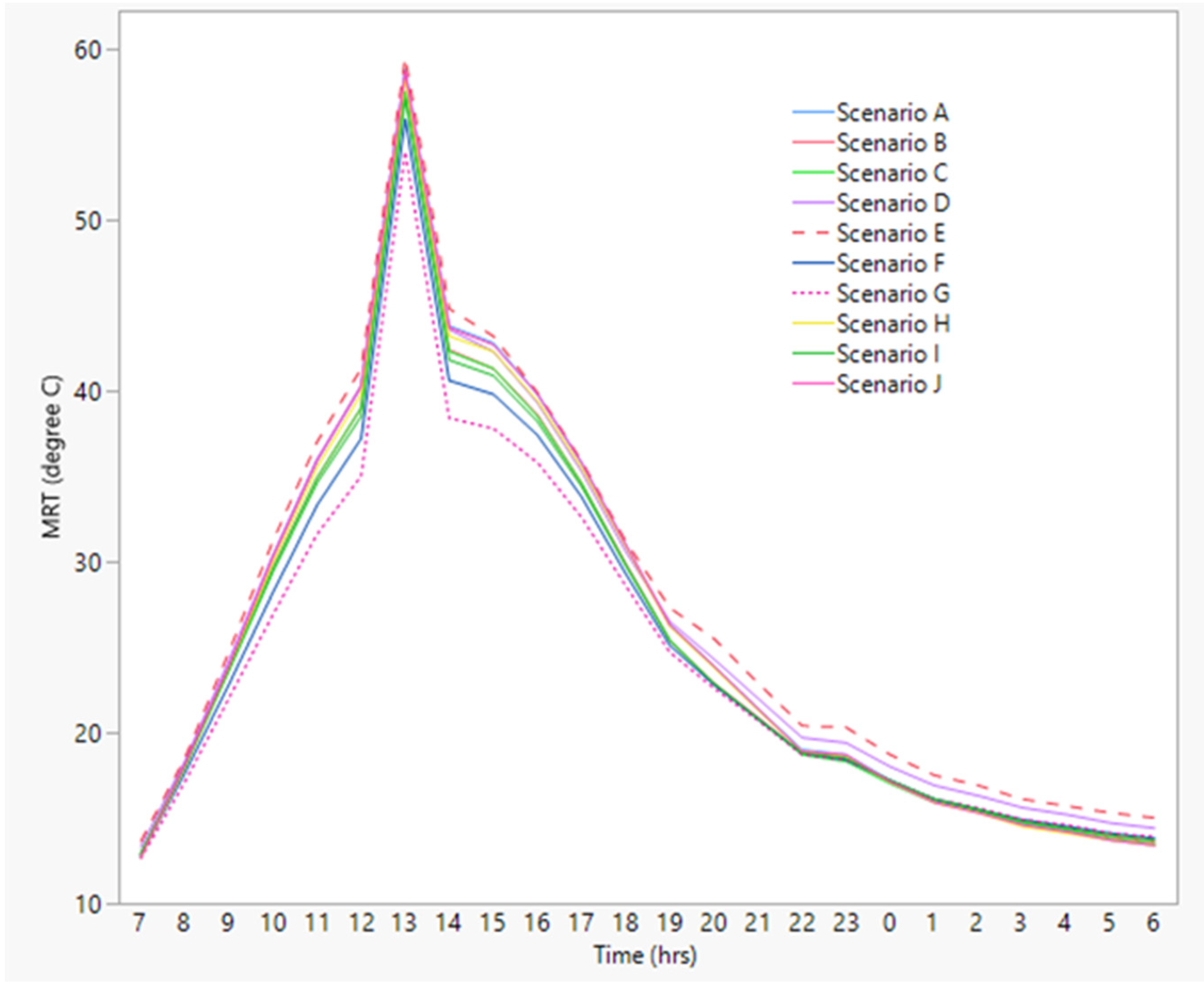
4.2. Mean Radiant Temperature

Mean radiant temperature (MRT) is a parameter that sums up the fluxes in shortwave and longwave radiation to which the human body is exposed. MRT is considered as an important meteorological parameter for the calculation of many human thermal comfort indices [57]. MRT in ENVI-met is calculated based on the following equation [70]:
T m r t = [ 1 σ ( E t ( z ) + α k ε ρ ( D t ( z ) + I t ( z ) ) ] 0.25
where σ, αk, and ερ are the Stefan–Boltzmann constant, a body’s total absorption coefficient for shortwave radiation and emissivity; Et(z), Dt(z) and It(z) are longwave, total diffuse shortwave and direct shortwave radiation flux absorbed by a body at height z, respectively. Figure 15 shows the hourly variation in MRT for different scenarios at point 19. In general, the profiles of MRT are qualitatively similar for all scenarios. During the day, MRT values reached the peak at around 13:00 and from 14:00 onwards, it dropped gradually. During the night and early morning, the MRT values were relatively low. It can be seen from the figure that the MRT values for Scenario E was the highest, whereas it was lowest for Scenario G.
Based on the simulation results, day time MRT of Scenarios B–J showed a maximum drop over base case within the time range of 12:00 to 16:00. Figure 16 provides MRT reduction for Scenarios B–J on 13 January at 15:00. Tree-based scenarios had the highest MRT reduction among all the scenarios with reductions by up to 7.6 °C and 5.5 °C for Scenarios G and F, respectively. Other scenarios resulted in moderate to small MRT reduction, with the smallest reduction being recorded in Scenarios H and J (0–0.1 °C).
MRT reduction are commonly associated with the tree’s foliage. The temperature is influenced by surface temperature of an open area which directly obtains solar radiation. Tree’s foliage plays an important role in reducing temperature as it provides protection from radiation by preventing solar radiation from hitting the ground and being reflected. Compared to trees, green roofs, green walls, pond and fountain scenarios were more exposed to solar radiation and, thus, the MRT reduction was also smaller in these scenarios. However, shading from high-rise buildings also contributes to reducing the MRT. This result is supported by previous research, which suggested that areas sheltered by either buildings or vegetation showed a significantly reduced MRT as compared to exposed areas [27,49,76]

4.3. Human Thermal Comfort

The following comfort analysis is based on physiological equivalent temperature (PET). The maximum and minimum PET values of Scenarios A–J at 15:00 were derived from the model (and presented in Table 4). In general, PET is maximum in all scenarios, except J; all of scenarios drop by 0.3–3.2 °C compared to base case (A). Maximum PET of tree scenarios (F and G) were 3.2 degrees lower than Scenario A while the minimum PET in Scenarios F and G drop by 3.4 °C and 2 °C, respectively. These maximum and minimum values were the most reduced among the scenarios. Maximum PET in water body and fountain scenarios (H and J) did not give noticeable difference as compared to the base case (Scenario A), while the maximum PET of the deeper water body scenario (Scenario I) reduced its value by 3 °C. Table 4 summarises the minimum and maximum PET values for Scenarios A–J.
Figure 17 presents the spatial distribution of PET for Scenarios A–J on 13 January at 15:00. It can be seen that the thermal perception for Scenario A was mostly hot (35–41 °C) and very hot (>41 °C). In general, green roofs and green walls have a small effect on improving the thermal comfort for the whole area. There was a small improvement in PET in some points in both Scenarios B and C. For example, point 19 in Scenario C experienced a PET drop by 0.9 °C (from 37.2 °C to 36.3 °C). Other points resulted in an average reduction by less than 1 °C. These reductions could not change the level of thermal perception from hot to warm. This strengthens the result from previous studies [17,18], which suggested that green roofs in high-rise building areas are not effective in improving the condition of thermal comfort at the pedestrian level. Similarly, Scenarios D and E also could not improve the level of thermal perception, although there were small reductions in PET at some points in Scenario E. Tree scenarios (F and G) showed considerable effects in improving thermal comfort of the environment, caused by significant reductions in both Ta and MRT. This is supported by previous research [16,17,68,74,77], which showed that the reduction in Ta and MRT improved thermal comfort, although the improvement was highly influenced by MRT (more than by Ta). As PET reduced significantly, the thermal perception was also improved from mostly hot to warm (Scenario G). Figure 18 shows a comparison of PET for Scenarios A, F and G at all the 28 points of observation. Scenario A (base case) experienced hot thermal perception. With application of tree scenario, four points in Scenario F and 18 points in Scenario G improved their thermal perception from hot to warm (<35 °C). Average reduction in PET were 2.0 °C and 3.6 °C in Scenarios F and G, respectively. Although many points in Scenario F could not reach a PET value of 35 °C (which is the minimum threshold for warm perception), the PET reduction as compared to the base case was considerably high.
Regarding water body (or BI) scenarios, there was no noticeable thermal comfort improvement in both Scenarios H and I as these scenarios could not improve the level of thermal perception from hot to warm. Even so, PET distribution in some areas in Scenario I was slightly better than that in Scenario H. There were some considerable MRT reduction in Scenario I (owing to shading from trees and buildings) which led to a reduction in PET. This result is in-line with a previous study [34], which found that the lower PET values in the research area came from tree shading around the water bodies, and not from the water bodies themselves. The fountains (in Scenario J) were found to not improve the thermal comfort condition. There was a temperature reduction at some points around the fountains, which ranged from 0.2–1.48 °C. However, these reductions were not followed by reduction in MRT, which is strongly associated with the human energy balance. In this scenario, there was no radiant heat loss and thus it counterbalanced the reduction in temperature in the area.
Among the simulated blue-green infrastructure scenarios, the tree-based ones clearly outperform others in providing a cooling effect and, hence, enhancing the thermal comfort. Apart from this, blue-green infrastructure is also widely known to provide other benefits such as managing stormwater runoff, improving air quality, encouraging biodiversity in an urban area, making urban environments more attractive and providing opportunities for relaxation and recreation. A previous study [78] showed blue-green infrastructure to potentially enhance natural capital and contribute to other forms of capital essential for the well-being of urban dwellers. Given the benefit they provide (other than the cooling effect), blue-green infrastructure is worth implementing in urban areas to tackle various other issues arising from urbanization and increasing population.
The benefits and ecosystem services provided by trees and other green spaces in the urban environment are well-known [77] and, hence, various types of GI have been widely included in urban planning in many cities, including Melbourne. For example, Plan Melbourne 2017–2050 outlines the vision of making Melbourne a sustainable and resilient city. The plan’s strategic statement identifies an urban forest of trees as a main strategy to make Melbourne cooler and greener. To achieve the aim, the City of Melbourne will maintain and enhance its urban forests of trees and vegetation on properties, lining transport corridors, public lands and on roofs, facades and walls.

5. Conclusions

Based on the analysis undertaken in this study, the key conclusions, observations and recommendations are as follows:
  • Green roofs and green walls in a high-rise building environments, such as the one considered in this study, have a small improvement in the microclimate of its surroundings. Since the improvements were too small, the aforementioned infrastructure cannot improve the level of thermal comfort during hot periods.
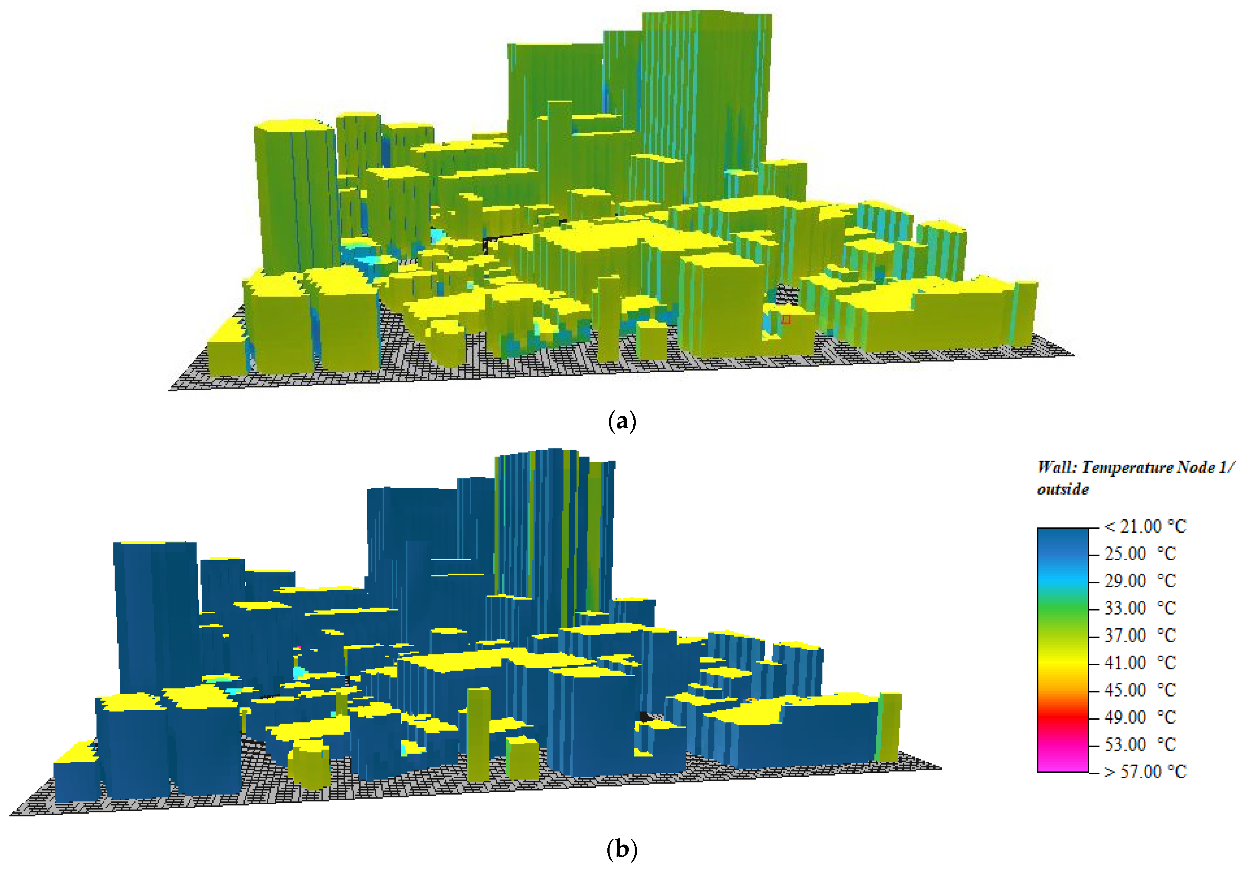
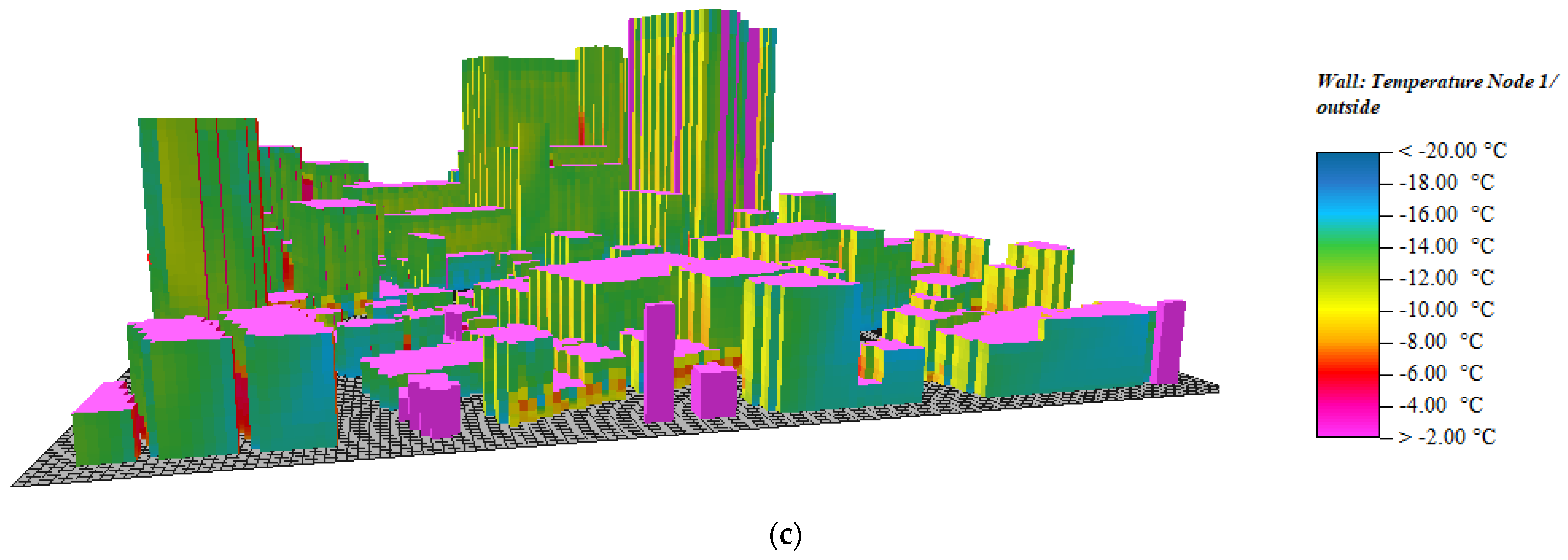
  • Although green walls cannot improve outdoor thermal comfort, the infrastructure is able to reduce the surface temperature of building walls, thus potentially reducing indoor temperature.
  • Trees in general have quite a significant cooling effect on the urban environment, and thus they can improve the level of thermal comfort. Shading, either by trees or buildings play an important role in improving the thermal comfort because it reduces the incoming short wave radiation reaching ground level, particularly at midday in the summer months when deciduous trees are full of leaves.
  • While water bodies do not bring a significant temperature reduction, implementing them can still create a cooler urban environment, especially with the deeper ones. It is shown from the simulation results that the 100 cm deep ponds have a better cooling effect than the 50 cm deep ponds.
  • Fountains can reduce air temperature quite significantly. However, as this is not followed by a reduction in the MRT, this strategy cannot improve thermal comfort. In addition, the cooling effect of fountains tends to be quite local. A noticeable reduction in Ta only occurred at a distance of less than 30 m from the fountain.
  • Green roofs and green walls are often considered as the most appropriate green infrastructure to mitigate the effects of rising temperatures, especially in an urban setting where the open spaces are limited. However, the simulation results from this study has shown that the outdoor cooling capability of green roofs and green walls in a high-rise and dense urban area is very small and, hence, it can almost be neglected. Nonetheless, green roofs and green walls in urban areas are still worth implementing, considering the host of other benefits that they provide.

Author Contributions

Conceptualization, F.B., N.M., A.W.M.N., S.M. and M.S.W.; methodology, F.B., N.M., A.W.M.N., S.M. and M.S.W.; writing—original draft preparation, F.B.; writing—review and editing, F.B., A.W.M.N., N.M., S.M. and M.S.W.; supervision, A.W.M.N., N.M., S.M. and M.S.W.; project administration, F.B.; funding acquisition, A.W.M.N., N.M., S.M. and M.S.W. All authors have read and agreed to the published version of the manuscript.

Funding

The first author received an Australia Awards Scholarship for undertaking this research. The project also received a ‘Green our Rooftop Demonstration Green Roof Collaborative Research Grant’ from the City of Melbourne (Grant no. GOR0252019), Melbourne, Australia. M.S. Wong received funding support from the General Research Fund (Grant No. 15603920 and 15609421), and the Collaborative Research Fund (Grant No. C5062-21GF) from the Research Grants Council, Hong Kong, China.

Institutional Review Board Statement

Not applicable.

Informed Consent Statement

Not applicable.

Acknowledgments

The authors would like to acknowledge and thank City of Melbourne for the support provided for this study. M. S. Wong would like to thank the funding support provided by the Research Grants Council of Hong Kong, China.

Conflicts of Interest

The authors declare no conflict of interest.

References

  1. Seto, K.; Reenberg, A. Rethinking Global Land-Use in an Urban Era; MIT Press: Cambridge, MA, USA, 2014; Volume 14. [Google Scholar]
  2. Akbari, H.; Pomerantz, M.; Taha, H. Cool surfaces and shade trees to reduce energy use and improve air quality in urban areas. Sol. Energy 2001, 70, 295–310. [Google Scholar] [CrossRef]
  3. Czarnecka, M.; Nidzgorska-Lencewicz, J. Intensity of Urban Heat Island and Air Quality in Gdańsk during 2010 Heat Wave. Pol. J. Environ. Stud. 2014, 23, 329–340. [Google Scholar]
  4. Donovan, G.H.; Butry, D.T. The value of shade: Estimating the effect of urban trees on summertime electricity use. Energy Build. 2009, 41, 662–668. [Google Scholar] [CrossRef]
  5. Santamouris, M.; Cartalis, C.; Synnefa, A.; Kolokotsa, D. On the impact of urban heat island and global warming on the power demand and electricity consumption of buildings—A review. Energy Build. 2015, 98, 119–124. [Google Scholar] [CrossRef]
  6. Sarrat, C.; Lemonsu, A.; Masson, V.; Guedalia, D. Impact of urban heat island on regional atmospheric pollution. Atmos. Environ. 2006, 40, 1743–1758. [Google Scholar] [CrossRef]
  7. Benedict, M.A.; McMahon, E.T. Green infrastructure: Smart conservation for the 21st century. Renew. Resour. J. 2002, 20, 12–17. [Google Scholar]
  8. Karakounos, I.; Dimoudi, A.; Zoras, S. The influence of bioclimatic urban redevelopment on outdoor thermal comfort. Energy Build. 2018, 158, 1266–1274. [Google Scholar] [CrossRef]
  9. Imhof, R.; De Jesus, M.; Xiao, P.; Ciortea, L.; Berg, E. Closed-chamber transepidermal water loss measurement: Microclimate, calibration and performance. Int. J. Cosmet. Sci. 2009, 31, 97–118. [Google Scholar] [CrossRef]
  10. Jamei, E.; Rajagopalan, P. Urban development and pedestrian thermal comfort in Melbourne. Sol. Energy 2017, 144, 681–698. [Google Scholar] [CrossRef]
  11. Jamei, E.; Sachdeva, H.; Rajagopalan, P. CBD greening and air temperature variation in Melbourne. In Proceedings of the 30th International PLEA Conference: Sustainable Habitat for Developing Societies, Choosing the Way Forward, Ahmedabad, India, 16–18 December 2014; CEPT University Press: Ahmedabad, India, 2014; pp. 123–132. [Google Scholar]
  12. Balany, F.; Ng, A.W.; Muttil, N.; Muthukumaran, S.; Wong, M.S. Green Infrastructure as an Urban Heat Island Mitigation Strategy—A Review. Water 2020, 12, 3577. [Google Scholar] [CrossRef]
  13. Feyisa, G.L.; Dons, K.; Meilby, H. Efficiency of parks in mitigating urban heat island effect: An example from Addis Ababa. Landsc. Urban Plan. 2014, 123, 87–95. [Google Scholar] [CrossRef]
  14. Razzaghmanesh, M.; Beecham, S.; Salemi, T. The role of green roofs in mitigating Urban Heat Island effects in the metropolitan area of Adelaide, South Australia. Urban For. Urban Green. 2016, 15, 89–102. [Google Scholar] [CrossRef]
  15. Shashua-Bar, L.; Pearlmutter, D.; Erell, E. The cooling efficiency of urban landscape strategies in a hot dry climate. Landsc. Urban Plan. 2009, 92, 179–186. [Google Scholar] [CrossRef]
  16. Lee, H.; Mayer, H.; Chen, L. Contribution of trees and grasslands to the mitigation of human heat stress in a residential district of Freiburg, Southwest Germany. Landsc. Urban Plan. 2016, 148, 37–50. [Google Scholar] [CrossRef]
  17. Perini, K.; Magliocco, A. Effects of vegetation, urban density, building height, and atmospheric conditions on local temperatures and thermal comfort. Urban For. Urban Green. 2014, 13, 495–506. [Google Scholar] [CrossRef]
  18. Ng, E.; Chen, L.; Wang, Y.; Yuan, C. A study on the cooling effects of greening in a high-density city: An experience from Hong Kong. Build. Environ. 2012, 47, 256–271. [Google Scholar] [CrossRef]
  19. Zhao, T.; Fong, K. Characterization of different heat mitigation strategies in landscape to fight against heat island and improve thermal comfort in hot–humid climate (Part I): Measurement and modelling. Sustain. Cities Soc. 2017, 32, 523–531. [Google Scholar] [CrossRef]
  20. Yu, C.; Hien, W.N. Thermal benefits of city parks. Energy Build. 2006, 38, 105–120. [Google Scholar] [CrossRef]
  21. Chang, C.-R.; Li, M.-H. Effects of urban parks on the local urban thermal environment. Urban For. Urban Green. 2014, 13, 672–681. [Google Scholar] [CrossRef]
  22. Mahmoud, A.H.A. Analysis of the microclimatic and human comfort conditions in an urban park in hot and arid regions. Build. Environ. 2011, 46, 2641–2656. [Google Scholar] [CrossRef]
  23. Morakinyo, T.E.; Lam, Y.F. Simulation study on the impact of tree-configuration, planting pattern and wind condition on street-canyon’s micro-climate and thermal comfort. Build. Environ. 2016, 103, 262–275. [Google Scholar] [CrossRef]
  24. Rui, L.; Buccolieri, R.; Gao, Z.; Ding, W.; Shen, J. The impact of green space layouts on microclimate and air quality in residential districts of Nanjing, China. Forests 2018, 9, 224. [Google Scholar] [CrossRef] [Green Version]
  25. Chow, W.T.; Brazel, A.J. Assessing xeriscaping as a sustainable heat island mitigation approach for a desert city. Build. Environ. 2012, 47, 170–181. [Google Scholar] [CrossRef]
  26. Kukal, M.S.; Irmak, S. Climate-driven crop yield and yield variability and climate change impacts on the US great plains agricultural production. Sci. Rep. 2018, 8, 3450. [Google Scholar] [CrossRef] [Green Version]
  27. Armson, D.; Rahman, M.A.; Ennos, A.R. A comparison of the shading effectiveness of five different street tree species in Manchester, UK. Arboric. Urban For. 2013, 39, 157–164. [Google Scholar] [CrossRef]
  28. Streiling, S.; Matzarakis, A. Influence of single and small clusters of trees on the bioclimate of a city: A case study. J. Arboric. 2003, 29, 309–316. [Google Scholar] [CrossRef]
  29. Chellamani, P.; Singh, C.P.; Panigrahy, S. Assessment of the health status of Indian mangrove ecosystems using multi temporal remote sensing data. Trop. Ecol. 2014, 55, 245–253. [Google Scholar]
  30. Symes, P.; Connellan, G. Water management strategies for urban trees in dry environments: Lessons for the future. Arboric. Urban For. 2013, 39, 116–124. [Google Scholar] [CrossRef]
  31. O’Donnell, E.C.; Thorne, C.R.; Yeakley, J.A.; Chan, F.K.S. Sustainable flood risk and stormwater management in blue-green cities; an interdisciplinary case study in Portland, Oregon. JAWRA J. Am. Water Resour. Assoc. 2020, 56, 757–775. [Google Scholar] [CrossRef]
  32. Ghofrani, Z.; Sposito, V.; Faggian, R. A comprehensive review of blue-green infrastructure concepts. Int. J. Environ. Sustain. 2017, 6, 15–36. [Google Scholar] [CrossRef]
  33. Spronken-Smith, R.A.; Oke, T.R.; Lowry, W.P. Advection and the surface energy balance across an irrigated urban park. Int. J. Climatol. A J. R. Meteorol. Soc. 2000, 20, 1033–1047. [Google Scholar] [CrossRef]
  34. Jacobs, C.; Klok, L.; Bruse, M.; Cortesão, J.; Lenzholzer, S.; Kluck, J. Are urban water bodies really cooling? Urban Clim. 2020, 32, 100607. [Google Scholar] [CrossRef]
  35. Du, H.; Song, X.; Jiang, H.; Kan, Z.; Wang, Z.; Cai, Y. Research on the cooling island effects of water body: A case study of Shanghai, China. Ecol. Indic. 2016, 67, 31–38. [Google Scholar] [CrossRef]
  36. Oláh, A. The possibilities of decreasing the urban heat island. Appl. Ecol. Environ. Res. 2012, 10, 173–183. [Google Scholar] [CrossRef]
  37. Sun, R.; Chen, A.; Chen, L.; Lü, Y. Cooling effects of wetlands in an urban region: The case of Beijing. Ecol. Indic. 2012, 20, 57–64. [Google Scholar] [CrossRef]
  38. Saaroni, H.; Ben-Dor, E.; Bitan, A.; Potchter, O. Spatial distribution and microscale characteristics of the urban heat island in Tel-Aviv, Israel. Landsc. Urban Plan. 2000, 48, 1–18. [Google Scholar] [CrossRef]
  39. Kim, Y.-H.; Ryoo, S.-B.; Baik, J.-J.; Park, I.-S.; Koo, H.-J.; Nam, J.-C. Does the restoration of an inner-city stream in Seoul affect local thermal environment? Theor. Appl. Climatol. 2008, 92, 239–248. [Google Scholar] [CrossRef]
  40. Inard, C.; Groleau, D.; Musy, M. Energy balance study of water ponds and its influence on building energy consumption. Build. Serv. Eng. Res. Technol. 2004, 25, 171–182. [Google Scholar] [CrossRef] [Green Version]
  41. Xue, F.; Li, X.; Ma, J.; Zhang, Z. Modeling the influence of fountain on urban microclimate. In Building Simulation; Springer: New York, NY, USA, 2015; pp. 285–295. [Google Scholar]
  42. Montazeri, H.; Toparlar, Y.; Blocken, B.; Hensen, J. Simulating the cooling effects of water spray systems in urban landscapes: A computational fluid dynamics study in Rotterdam, The Netherlands. Landsc. Urban Plan. 2017, 159, 85–100. [Google Scholar] [CrossRef]
  43. Coutts, A.M.; Tapper, N.J.; Beringer, J.; Loughnan, M.; Demuzere, M. Watering our cities: The capacity for Water Sensitive Urban Design to support urban cooling and improve human thermal comfort in the Australian context. Prog. Phys. Geogr. 2013, 37, 2–28. [Google Scholar] [CrossRef]
  44. Broadbent, A.M.; Coutts, A.M.; Nice, K.A.; Demuzere, M.; Krayenhoff, E.S.; Tapper, N.J.; Wouters, H. The Air-temperature Response to Green/blue-infrastructure Evaluation Tool (TARGET v1. 0): An efficient and user-friendly model of city cooling. Geosci. Model Dev. 2019, 12, 785–803. [Google Scholar] [CrossRef] [Green Version]
  45. Well, F.; Ludwig, F. Development of an Integrated Design Strategy for Blue-Green Architecture. Sustainability 2021, 13, 7944. [Google Scholar] [CrossRef]
  46. Caborn, J.M. Shelterbelts and Microclimate; HM Stationery Office Edinburgh: London, UK, 1957.
  47. Te Kulve, M.; Schlangen, L.; van Marken Lichtenbelt, W. Interactions between the perception of light and temperature. Indoor Air 2018, 28, 881–891. [Google Scholar] [CrossRef] [Green Version]
  48. Tiller, D.; Wang, L.M.; Musser, A.; Radik, M. AB-10-017: Combined Effects of Noise and Temperature on Human Comfort and Performance (1128-RP); University of Nebraska-Lincoln: Lincoln, NE, USA, 2010; Available online: https://digitalcommons.unl.edu/archengfacpub/40 (accessed on 24 May 2022).
  49. Ali-Toudert, F.; Mayer, H. Numerical study on the effects of aspect ratio and orientation of an urban street canyon on outdoor thermal comfort in hot and dry climate. Build. Environ. 2006, 41, 94–108. [Google Scholar] [CrossRef]
  50. Müller, N.; Kuttler, W.; Barlag, A.-B. Counteracting urban climate change: Adaptation measures and their effect on thermal comfort. Theor. Appl. Climatol. 2014, 115, 243–257. [Google Scholar] [CrossRef] [Green Version]
  51. Lobaccaro, G.; Acero, J.A. Comparative analysis of green actions to improve outdoor thermal comfort inside typical urban street canyons. Urban Clim. 2015, 14, 251–267. [Google Scholar] [CrossRef]
  52. Chen, Y.-C.; Matzarakis, A. Modified physiologically equivalent temperature—Basics and applications for western European climate. Theor. Appl. Climatol. 2018, 132, 1275–1289. [Google Scholar] [CrossRef]
  53. Johansson, E.; Thorsson, S.; Emmanuel, R.; Krüger, E. Instruments and methods in outdoor thermal comfort studies–The need for standardization. Urban Clim. 2014, 10, 346–366. [Google Scholar] [CrossRef] [Green Version]
  54. Perini, K.; Chokhachian, A.; Dong, S.; Auer, T. Modeling and simulating urban outdoor comfort: Coupling ENVI-Met and TRNSYS by grasshopper. Energy Build. 2017, 152, 373–384. [Google Scholar] [CrossRef]
  55. Blazejczyk, K.; Epstein, Y.; Jendritzky, G.; Staiger, H.; Tinz, B. Comparison of UTCI to selected thermal indices. Int. J. Biometeorol. 2012, 56, 515–535. [Google Scholar] [CrossRef] [Green Version]
  56. Taleghani, M.; Kleerekoper, L.; Tenpierik, M.; van den Dobbelsteen, A. Outdoor thermal comfort within five different urban forms in the Netherlands. Build. Environ. 2015, 83, 65–78. [Google Scholar] [CrossRef]
  57. Höppe, P. The physiological equivalent temperature–a universal index for the biometeorological assessment of the thermal environment. Int. J. Biometeorol. 1999, 43, 71–75. [Google Scholar] [CrossRef] [PubMed]
  58. Lin, T.-P.; Yang, S.-R.; Chen, Y.-C.; Matzarakis, A. The potential of a modified physiologically equivalent temperature (mPET) based on local thermal comfort perception in hot and humid regions. Theor. Appl. Climatol. 2019, 135, 873–876. [Google Scholar] [CrossRef]
  59. Rajagopalan, P.; Lim, K.C.; Jamei, E. Urban heat island and wind flow characteristics of a tropical city. Sol. Energy 2014, 107, 159–170. [Google Scholar] [CrossRef]
  60. Bruse, M.; Fleer, H. Simulating surface–plant–air interactions inside urban environments with a three dimensional numerical model. Environ. Model. Softw. 1998, 13, 373–384. [Google Scholar] [CrossRef]
  61. Skelhorn, C.; Lindley, S.; Levermore, G. The impact of vegetation types on air and surface temperatures in a temperate city: A fine scale assessment in Manchester, UK. Landsc. Urban Plan. 2014, 121, 129–140. [Google Scholar] [CrossRef]
  62. Oke, T.R.; Mills, G.; Christen, A.; Voogt, J.A. Urban Climates; Cambridge University Press: Cambridge, UK, 2017. [Google Scholar]
  63. Salata, F.; Golasi, I.; de Lieto Vollaro, R.; de Lieto Vollaro, A. Urban microclimate and outdoor thermal comfort. A proper procedure to fit ENVI-met simulation outputs to experimental data. Sustain. Cities Soc. 2016, 26, 318–343. [Google Scholar] [CrossRef]
  64. Acero, J.A.; Arrizabalaga, J. Evaluating the performance of ENVI-met model in diurnal cycles for different meteorological conditions. Theor. Appl. Climatol. 2018, 131, 455–469. [Google Scholar] [CrossRef]
  65. Santhi, C.; Arnold, J.G.; Williams, J.R.; Dugas, W.A.; Srinivasan, R.; Hauck, L.M. Validation of the swat model on a large rwer basin with point and nonpoint sources 1. JAWRA J. Am. Water Resour. Assoc. 2001, 37, 1169–1188. [Google Scholar] [CrossRef]
  66. Willmott, C.J. Some comments on the evaluation of model performance. Bull. Am. Meteorol. Soc. 1982, 63, 1309–1313. [Google Scholar] [CrossRef] [Green Version]
  67. Tsoka, S.; Tsikaloudaki, A.; Theodosiou, T. Analyzing the ENVI-met microclimate model’s performance and assessing cool materials and urban vegetation applications–A review. Sustain. Cities Soc. 2018, 43, 55–76. [Google Scholar] [CrossRef]
  68. Herath, H.; Halwatura, R.; Jayasinghe, G. Evaluation of green infrastructure effects on tropical Sri Lankan urban context as an urban heat island adaptation strategy. Urban For. Urban Green. 2018, 29, 212–222. [Google Scholar] [CrossRef]
  69. Kim, J.; Lee, S.Y.; Kang, J. Temperature Reduction Effects of Rooftop Garden Arrangements: A Case Study of Seoul National University. Sustainability 2020, 12, 6032. [Google Scholar] [CrossRef]
  70. Tsoka, S. Investigating the relationship between urban spaces morphology and local microclimate: A study for Thessaloniki. Procedia Environ. Sci. 2017, 38, 674–681. [Google Scholar] [CrossRef]
  71. Al-Kayiem, H.H.; Koh, K.; Riyadi, T.W.; Effendy, M. A Comparative Review on Greenery Ecosystems and Their Impacts on Sustainability of Building Environment. Sustainability 2020, 12, 8529. [Google Scholar] [CrossRef]
  72. Alexandri, E.; Jones, P. Temperature decreases in an urban canyon due to green walls and green roofs in diverse climates. Build. Environ. 2008, 43, 480–493. [Google Scholar] [CrossRef]
  73. Duarte, D.H.; Shinzato, P.; dos Santos Gusson, C.; Alves, C.A. The impact of vegetation on urban microclimate to counterbalance built density in a subtropical changing climate. Urban Clim. 2015, 14, 224–239. [Google Scholar] [CrossRef]
  74. Salata, F.; Golasi, I.; Petitti, D.; de Lieto Vollaro, E.; Coppi, M.; de Lieto Vollaro, A. Relating microclimate, human thermal comfort and health during heat waves: An analysis of heat island mitigation strategies through a case study in an urban outdoor environment. Sustain. Cities Soc. 2017, 30, 79–96. [Google Scholar] [CrossRef]
  75. Srivanit, M.; Hokao, K. Evaluating the cooling effects of greening for improving the outdoor thermal environment at an institutional campus in the summer. Build. Environ. 2013, 66, 158–172. [Google Scholar] [CrossRef]
  76. Tsoka, S.; Tsikaloudaki, K.; Theodosiou, T. Urban space’s morphology and microclimatic analysis: A study for a typical urban district in the Mediterranean city of Thessaloniki, Greece. Energy Build. 2017, 156, 96–108. [Google Scholar] [CrossRef]
  77. Rui, L.; Buccolieri, R.; Gao, Z.; Gatto, E.; Ding, W. Study of the effect of green quantity and structure on thermal comfort and air quality in an urban-like residential district by ENVI-met modelling. In Building Simulation; Springer: New York, NY, USA, 2019; pp. 183–194. [Google Scholar]
  78. Ncube, S.; Arthur, S. Influence of Blue-Green and Grey Infrastructure Combinations on Natural and Human-Derived Capital in Urban Drainage Planning. Sustainability 2021, 13, 2571. [Google Scholar] [CrossRef]
Figure 1. The research method used in the study.
Sustainability 14 09057 g001
Figure 2. An aerial view of Melbourne’s Central Business District (CBD).
Sustainability 14 09057 g002
Figure 3. A two-dimensional view of the research area.
Sustainability 14 09057 g003
Figure 4. A three-dimensional view of the research area.
Sustainability 14 09057 g004
Figure 5. Regression analysis between simulated and observed values of Ta.
Sustainability 14 09057 g005
Figure 6. Regression analysis between simulated and observed values of RH.
Sustainability 14 09057 g006
Figure 7. Layout of scenarios; (a) B, (b) C, (c) D, (d) E, (e) F, (f) G and (g) H/J.
Sustainability 14 09057 g007aSustainability 14 09057 g007b
Figure 8. Location of the 13 fountains.
Sustainability 14 09057 g008
Figure 9. Distribution of 28 points from where the results were extracted.
Sustainability 14 09057 g009
Figure 10. Temporal profile of Ta and RH for Scenarios A𠄲J at point 19.
Sustainability 14 09057 g010
Figure 11. Walls temperature; (a) Scenario A, (b) Scenario E, (c) the difference between Scenarios A and E.
Sustainability 14 09057 g011aSustainability 14 09057 g011b
Figure 12. Temperature reduction (as compared to the base case) for Scenarios B–J at 15:00.
Sustainability 14 09057 g012
Figure 13. The relationship between distance from the fountain and temperature reduction (from the base case) for scenario J.
Sustainability 14 09057 g013
Figure 14. Increase in relative humidity (as compared to the base case) for Scenarios B–J at 15:00.
Sustainability 14 09057 g014
Figure 15. Temporal profile of MRT for Scenarios A–J at point 19.
Sustainability 14 09057 g015
Figure 16. Reduction in MRT (as compared to the base case) for Scenarios B–J at 15:00.
Sustainability 14 09057 g016
Figure 17. Spatial distribution of PET for scenario A–J at 15:00.
Sustainability 14 09057 g017aSustainability 14 09057 g017bSustainability 14 09057 g017c
Figure 18. Comparison of PET for Scenarios A, F and G at the 28 points of observation.
Sustainability 14 09057 g018
Table 1. The configuration of the ENVI-met simulations.
LocationMelbourne CBD (37.814° S, 144.963° E)
Simulation starting period06:00, 12–14 January 2020
Total simulation time in hours *48 h
Save model state (each min) *60
Factor of short-wave adjustment1
Roughness length (Z0)2
Initial temperature, upper layer (0–20 cm; K)293
Initial temperature, middle layer (20–50 cm; k)293
Initial temperature, deep layer (>50 cm; k)293
Relative humidity, upper layer 30
Relative humidity, middle layer60
Relative humidity, deep layer 60
Albedo walls0.2
Albedo roofs0.3
Soil profileLoamy soil
Save receptor (each min) *60 min
* Total simulation time: total time needed to calculate; Save model state: time interval to write the model state to disk; Save receptor: selected points in model area that allow to collect data in a compact way with high resolution.
Table 2. Numerical threshold of PET.
Thermal PerceptionGrade of Physiological StressRange (°C)
Very coldExtreme cold stress<4
ColdStrong cold stress4–8
CoolModerate cold stress8–13
Slightly coolSlight cold stress13–18
ComfortableNo thermal stress18–23
Slightly warmSlight heat stress23–29
WarmModerate heat stress29–35
HotStrong heat stress35–41
Very hotExtreme heat stress>41
Table 3. Performance indicators for ENVI-met based on observed and simulated Ta and RH values.
ParameterR2RMSEd
Ta0.9272.070.948
RH0.88311.120.922
Table 4. Minimum and maximum values of PET for Scenarios A–J.
ScenarioPET (°C)
MinMax
A33.260.3
B32.357.6
C32.257.6
D33.259.0
E33.358.3
F31.257.0
G29.857.0
H32.160.0
I32.057.3
J33.260.3
Publisher’s Note: MDPI stays neutral with regard to jurisdictional claims in published maps and institutional affiliations.

