Article

Random Forest Estimation and Trend Analysis of PM2.5 Concentration over the Huaihai Economic Zone, China (2000–2020)

1
School of Public Policy and Management, China University of Mining and Technology, Daxue Road 1, Xuzhou 221116, China
2
Research Center for Transition Development and Rural Revitalization of Resource-Based Cities in China, China University of Mining and Technology, Xuzhou 221116, China
3
Collaborative Innovation Center for Territorial Space Safety & Management, China University of Mining and Technology, Xuzhou 221116, China
4
University of the Chinese Academy of Sciences, Beijing 100049, China
5
Department of Geography, Vrije Universiteit Brussel, Pleinlaan 2, 1050 Brussels, Belgium
*
Author to whom correspondence should be addressed.
These authors contributed equally to this work and should be considered as co-first authors.
Sustainability 2022, 14(14), 8520; https://doi.org/10.3390/su14148520
Submission received: 6 May 2022 / Revised: 7 July 2022 / Accepted: 8 July 2022 / Published: 12 July 2022

Abstract

:
Consisting of ten cities in four Chinese provinces, the Huaihai Economic Zone has suffered serious air pollution over the last two decades, particularly of fine particulate matter (PM2.5). In this study, we used multi-source data, namely MAIAC AOD (at a 1 km spatial resolution), meteorological, topographic, date, and location (latitude and longitude) data, to construct a regression model using random forest to estimate the daily PM2.5 concentration over the Huaihai Economic Zone from 2000 to 2020. It was found that the variable expressing time (date) had the greatest characteristic importance when estimating PM2.5. By averaging the modeled daily PM2.5 concentration, we produced a yearly PM2.5 concentration dataset, at a 1 km resolution, for the study area from 2000 to 2020. On comparing modeled daily PM2.5 with observational data, the coefficient of determination ( R 2 ) of the modeling was 0.85, the root means square error ( R M S E ) was 14.63 μg/m3, and the mean absolute error ( M A E ) was 10.03 μg/m3. The quality assessment of the synthesized yearly PM2.5 concentration dataset shows that R 2 = 0.77, R M S E = 6.92 μg/m3, and M A E = 5.42 μg/m3. Despite different trends from 2000–2010 and from 2010–2020, the trend of PM2.5 concentration over the Huaihai Economic Zone during the 21 years was, overall, decreasing. The area of the significantly decreasing trend was small and mainly concentrated in the lake areas of the Zone. It is concluded that PM2.5 can be well-estimated from the MAIAC AOD dataset, when incorporating spatiotemporal variability using random forest, and that the resultant PM2.5 concentration data provide a basis for environmental monitoring over large geographic areas.

Graphical Abstract

1. Introduction

PM2.5 has become a great threat to human health, increasing the risk of respiratory and cardiovascular diseases [1]. The World Health Organization (WHO) has reported that nearly 90% of global population breathe air exceeding WHO air quality limits [2,3]. It is estimated that air pollution has claimed 6.67 million deaths worldwide in 2019 [4] and nearly 2 million deaths in China every year [2], which makes air pollution the fourth largest risk factor for global mortality [4]. China’s 337 cities experienced a total of 345 days of severe pollution and 1152 days of serious pollution in 2020, with PM2.5 pollution accounting for 77.7% of days of serious pollution [5]. Due to the dispersion of air pollution from two neighboring regions (the Beijing-Tianjin-Hebei Region and the Yangtze River Delta Region (Figure 1a)), and severe air pollutant emissions of its own, the Huaihai Economic Zone has serious air pollution [6,7,8,9]. The air quality of the 10 cities in the Huaihai Economic Zone is lower than the national average level for the same period [10]. It is evident that the importance of air pollution in China and the Zone cannot be underestimated. However, no attempts have yet been made to estimate the PM2.5 concentration specifically over this large area and examine its spatiotemporal evolution for a long period.
Traditionally, PM2.5 is observed at ground-based sites. Due to the limited number and uneven distribution of ground-based sites, PM2.5 data generally tend to have low spatial coverage. Additionally, the ground-based monitoring network was built quite late in China and there is an absence of long-term PM2.5 data records [11], which hinders PM2.5 studies that rely on time-series data. Such issues can however be addressed using remote sensing observations. PM2.5 can be inferred from aerosol optical depth (AOD) data, due to the correlation between AOD and PM2.5 [12]. Satellite-derived AOD data have a wide spatial coverage and high temporal and spatial resolutions, providing an effective way to monitor near-ground PM2.5 concentration and address the spatial discontinuity of ground-based PM2.5 data [13,14]. The correlation between satellite-derived AOD data and PM2.5 concentration data allows the mapping of PM2.5 concentration at reliable levels of accuracy and continuous spatial coverage, which is crucial for characterizing the spatial variability of PM2.5 concentration and formulating a context-specific, rather than one-size-fits-all, air pollution control policy [15].
AOD-based PM2.5 estimation methods can be roughly divided into three categories, namely, empirical statistical methods, chemical transfer models, and vertical correction models. The chemical transfer models are more data-demanding and more influenced by uncertainties in emission inventories and model parameters, and the vertical revision method does not account for the vertical stratification structure of PM2.5. Compared with these two methods, empirical statistical models are considered to be simpler, faster, and more accurate [16]. In empirical statistics methods, machine learning is considered more effective in addressing the relationships between variables with high autocorrelation and complex interactions than traditional linear regression models [17]. Machine learning can better handle large volumes of multi-dimensional and multi-variety data and more easily discover trends and patterns from time series data than traditional methods [18,19]. As one of the most popular machine learning methods, random forest is generally recognized as superior to other machine learning regression models because it assumes no normality, is faster and easier to run, returns feature importance, and possesses better prediction accuracy [18,19,20,21]. Therefore, it has been widely used for various purposes, such as disease prediction [22], risk assessment [23,24], and PM2.5 concentration estimation [20,25,26].
In previous studies on machine learning modeling of PM2.5 concentration, auxiliary variables other than AOD fall into the following categories: meteorological parameters [27,28,29,30,31,32], land use types [28,30], topography [32], and other associated pollutant factors [31]. Since PM2.5 concentration has seasonal differences [33] and spatial autocorrelation [34,35], the influences of time and geographical location on PM2.5 concentration should be considered in the process of modeling PM2.5 concentration at a 1 km resolution. In order to improve estimation accuracy, this study intends to take the spatiotemporal heterogeneity of PM2.5 concentration into account by adding date, latitude, and longitude as extra predictor variables.
This study focuses on the estimation of daily PM2.5 concentration from the 1-km resolution MAIAC AOD dataset over the Huaihai Economic Zone during 2000–2020. The specific objectives of this study are: (1) testing random forest for modeling daily PM2.5 concentration at a 1 km resolution by combining AOD, meteorological, topographic, date, and location data, (2) producing a yearly PM2.5 concentration dataset at a 1 km resolution for the study area from 2000–2020 by averaging the model daily PM2.5 concentration data and assessing its quality, and (3) unraveling the trend of PM2.5 concentration in the study area over the 21 years.

2. Data and Methods

2.1. Study Area

Among the earliest regional economic cooperation organizations in China, the Huaihai Economic Zone was established in 1986 and initially involved 20 cities in the Shandong, Jiangsu, Henan, and Anhui provinces. Xuzhou has been officially assigned as the central city of the zone by the State Council of China [36]. In November 2018, China confirmed that the zone consists of 10 major prefectural cities (Figure 1b), 3 Jiangsu cities (Xuzhou, Lianyungang, and Suqian), 4 Shandong cities (Zaozhuang, Linyi, Heze, and Jining), 1 Henan city (Shangqiu), and 2 Anhui cities (Huaibei and Suzhou) [37].
The climate in the zone belongs to the typical temperate continental monsoon climate that is characterized by distinct seasons, with a hot, rainy summer (June–August) and a cold, dry winter (December–February). The elevation is low in the south and high in the north, with an average elevation of 63.02 m. In total, the zone covers a geographical area of 95,805 km2 and a population of over 72.61 million. Among the 10 cities, Xuzhou, Suqian, Zaozhuang, Jining, Huaibei, and Suzhou are resource-based cities and there has long been concern over their air pollution issues. The rapid socioeconomic development in the zone, particularly urban expansion and population growth, in the last two decades, has further lowered the regional air quality.

2.2. Data

2.2.1. Ground-Observed PM2.5 Data

In the study area, there are 79 monitoring sites recording PM2.5 data (Figure 1b), as part of the China Environmental Monitoring Station. These sites provide hourly PM2.5 concentration data over the study area. As MODIS satellites pass the study area from 10 a.m. to 2 p.m., hourly PM concentration data during these five hours were selected for this study (Table 1). The selected hourly PM2.5 concentration data were averaged as the observed daily PM2.5 concentration.

2.2.2. AOD Data

The AOD data used in this study were derived from the MCD19A1 Version 6 data product, a Moderate Resolution Imaging Spectroradiometer (MODIS) Terra and Aqua combined Multi-angle Implementation of Atmospheric Correction (MAIAC) Land AOD gridded Level 2 product, produced daily at a 1 km resolution [38]. Compared with other AOD products (e.g., the 10-km-resolution DB AOD and 3-km-resolution DT AOD [39]), MAIAC AOD products have a higher spatial resolution, which better characterizes the spatial heterogeneity of AOD and therefore benefits the estimation of PM2.5 concentration. The AOD data downloaded consist of both Aqua and Terra AOD data, which were averaged as the daily AOD data. In total, we downloaded 7567 AOD images over the entire study area and 7567 days of the period from 1 January 2000 to 31 December 2020 (i.e., 7670 days), with a high temporal coverage of 98.66%. For the spatial coverage, we did not complete AOD data because the impact of the missing AOD data is limited [26,39,40] on yearly PM2.5 concentration products; furthermore, data completion does not lead to significantly improved spatial coverage [26,40,41] on yearly PM2.5 concentration products but induces errors that undermine model evaluation [39,42].
In order to match PM2.5 measurements with AOD data, we extracted AOD values in the 1-km AOD image data at the locations of PM2.5 monitoring sites using the ‘Extracting Values to Points’ utility in ArcGIS, which helped to identify a total of 5237 pairs of matched PM2.5 measurements and AOD data. After matching the ground-observed PM2.5 data to the obtained AOD data and removing the data pair containing the missing AOD values, a total of 5237 pairs of matched PM2.5 and AOD data were obtained. Meteorological, topographic, date, and location data were similarly matched with these pairs for modeling. The matched 5273 data records in 2020 were used to build an estimation model of PM2.5 concentration, and the daily PM2.5 concentration data in 2019 were averaged as the observed yearly PM2.5 concentration (79 samples) to assess the quality of the synthesized yearly PM2.5 concentration dataset (Section 2.3.3).

2.2.3. Meteorological Data

ERA5 is the fifth-generation ECMWF (European Centre for Medium-Range Weather Forecasts) atmospheric reanalysis of the global climate, covering the period from January 1950 to the present. The family of ERA5 datasets consists of ERA5 (a comprehensive reanalysis from 1979 to near real-time), ERA5.1 (a re-run of EAR5 for the years 2000 to 2006 only), and ERA5-Land (a land surface dataset from 1950 to the present time). In this study, because our study focuses on land and requires finer details, we used the ERA5-Land dataset. ERA5-Land provides hourly, high-resolution information of surface variables over several decades at a ~9 km grid spacing and covers the period from 1950 to 2–3 months before the present [43]. More information about ERA5 can be found on its official website [44].
Previous studies have shown that there are significant spatial differences in the effect of meteorological conditions on PM2.5 concentration. In order to construct a PM2.5 concentration estimation model applicable to this study area, we selected the four meteorological variables with the strongest importance for PM2.5 estimation in our region, according to Jing et al. [45], and added boundary-layer height as the fifth meteorological variable due to its widely proven importance [46,47,48].
The meteorological data used in this study were extracted from the ERA5-Land hourly data from 1950 to the present, including 10 m_U wind speed (the eastward wind component at a height of 10 m above the surface of land), 10 m_V wind speed (the northward wind component at a height of 10 m above the surface of land), 2 m temperature (air temperature at a height of 2 m above the surface of land), boundary-layer height (the height of the planetary boundary layer, the lowest part of the troposphere and the closest to Earth’s surface), near-surface pressure, and total precipitation (Table 1).
As the downloaded meteorological data are in Network Common Data Form (NetCDF) format at a 0.1° spatial resolution, they were converted into raster data in the TIFF format and resampled to the spatial resolution of AOD data (i.e., 1 km) using the bilinear interpolation method. Using the same method as that described in Section 2.2.2, we matched the meteorological data to the corresponding AOD data. In order to have the same passing time of the Terra and Aqua satellites, the hourly meteorological data acquired from 10 am to 2 pm was averaged and used to represent daily meteorological conditions. As such, five different variables were derived from these data, namely wind speed (WS, which is the vector addition of 10 m_U wind speed and 10 m_V wind speed), 2 m temperature (T2M), boundary-layer height (BLH), near-surface pressure (SP), and total precipitation (TP).

2.2.4. Topographic Data

As Zhang et al. [49] have shown that topography can intensify PM2.5 pollution, we used surface elevation (SE) to consider the topographic effect on PM2.5 concentration. Elevation data used in this study were extracted from the SRTM (Shuttle Radar Topography Mission) DEM (digital elevation model) dataset (Table 1). The spatial resolution of the dataset is 90 m, but it was resampled to the spatial resolution of AOD data (i.e., 1 km). Using the same method as that described in Section 2.2.2, we matched the topographic data to the AOD data.

2.2.5. Date and Location Data

As the PM2.5 concentration is associated with seasonal change and geographical location, we considered these factors by introducing appropriate variables. When a PM2.5 concentration was observed at the monitoring sites, the order of the date within the year could help transform the date into a numeric variable for modeling (Table 1). For example, 1 January was treated as value 1 and 31 December as value 365. Regarding the geographic location, the longitude and latitude of the center of each pixel was used to create a variable for longitude and a variable for latitude.

2.3. Methods

2.3.1. Pearson Correlation Analysis

In order to understand how the observed PM2.5 is correlated with the selected variables, a Pearson correlation analysis was performed [13]. This would provide a basis for the modeling of PM2.5. The data used for the correlation analysis had been matched with AOD data in 2020 (Section 2.2). The Pearson correlation analysis was performed on 5237 samples. Table 2 shows the results of the Pearson correlation analysis. Except for TP, all the other variables were significantly correlated with PM2.5 and therefore selected as the variables for modeling.

2.3.2. Random Forest Modeling

Random forest was used to estimate daily PM2.5 concentrations with the nine variables (features) determined in Section 2.3.1. Random forest is an ensemble learning method for the classification and regression method, based on a large number of different and independent decision trees [50,51]. Each decision tree in the forest returns a prediction and the average of all the predictions is treated as the prediction of the forest [50]. It can efficiently process a substantial number of input features (variables) and assess the importance of each. It is generally believed that random forest outperforms linear algorithms, such as linear and logistic regression [20,25]. In addition, random forest can evaluate the importance of features entering the forest, which facilitates the analysis of predictor variables. More information about how random forest is used for regression is detailed in previous studies [52,53].
There are two key parameters to be tuned in the application of random forest, namely, the number of decision trees (n_estimators) and the number of features randomly selected at each node (max_features) [51]. The values for n_estimators to be selected range from 100 to 5000 with increments of 100. As too many trees are computationally expensive and do not necessarily produce better results [50,54], we did not exceed 5000 trees. The values for max_features to be selected consists of p (where p is the number of available features/variables), p / 2 , and 2 p , which is recommended by the developer of random forest [51,55]. In this study, these values are 2, 3, and 6, respectively, since there are 9 variables.
In order to identify optimal values for the two parameters(n_estimators and max_features), we made use of GridSearchCV, a tool that tunes the parameters of a machining learning model using the grid-search and k-fold cross-validation techniques [56]. For two parameters, grid search uses different combinations of their possible values, calculates the performance for each value combination, and selects the value combination with the best performance for the parameters. This process is realized by the k-fold cross-validation, which helps to evaluate the quality of a model and select a model that performs best on unseen data [57]. The data from 2020 were used to build the daily PM2.5 concentration estimation model (Section 2.2.2) and were randomly split into two parts: 70% were used as training data (3691 samples) for training the random forest model and 30% were used as testing data (1582 samples) for evaluating the model. The 70/30 proportion for splitting data for training and testing is recommended by and used in many studies [58,59,60]. The training data were further divided into k equally sized folds (or sets). We used each as the validation set and the other k − 1 folds as the training set, fitted a random forest model with the training set, calculated the accuracy of the model with the validation set, and averaged the accuracies derived in each cross-validation. We repeated the procedure k times and obtain k average accuracies. The value combination that has the highest averaged accuracy was selected as the optimal values for the two parameters. In this study, the coefficient of determination (R²) was used to measure the model’s accuracy. According to method suggested by Jung [61] for selecting the optimal k value for cross validation, k = 8 was used.
After parameter tuning, a final random forest model for daily PM2.5 concentration estimation was determined. The model was then applied to the test data, which were never used in the modeling, for evaluating the model with coefficient of determination ( R 2 ), root mean square error ( R M S E ), and mean absolute error ( M A E ) [62,63,64].
R 2 = 1 i = 1 n y i ^ y i 2 i = 1 n y i y ¯ 2
R M S E = Σ i = 1 n y ^ i y i 2 n
M A E = i = 1 n y ^ i y i n
where y i ^ is the ground observation, y i   is the model estimate, y ¯   is the average of y i , and n is the sample size.

2.3.3. Yearly PM2.5 Concentration Dataset

By applying the determined daily PM2.5 concentration estimation model, we were able to produce a daily PM2.5 concentration dataset at a 1 km resolution. By averaging the daily PM2.5 concentration dataset, a yearly PM2.5 concentration dataset of the Huaihai Economic Zone from 2000 to 2020 was then synthesized. The yearly PM2.5 concentration dataset can provide a basis for the spatiotemporal evolution analysis of PM2.5 concentration over the study area during the two decades. It is noted that due to the presence of cloud, snow, and ice, AOD data are not available for every pixel for every single day of a year. This means that not every single pixel in the yearly dataset was based on 365 (or 366) days’ PM2.5 concentration. As such, it is necessary to conduct a data quality assessment of the synthesized yearly PM2.5 concentration dataset before its deployment in applications such as spatiotemporal analysis. Since not all the data from 2000 to 2019 were used in the model training, we should conduct the data quality assessment on the synthesized yearly PM2.5 concentration data from the rest years. Because the monitoring sites in the study area became available only as of 13 May 2014, and the number of available sites available varied from year to year, hourly PM2.5 concentration data (10 am to 2 pm) from the available PM2.5 monitoring sites from 2015 to 2020 were averaged, respectively, as the observed yearly PM2.5 concentration data from 2015 to 2020. Values at the locations of the PM2.5 monitoring sites were extracted from the synthesized yearly PM2.5 concentration data from 2015 to 2020 as the modeled yearly PM2.5 concentration data. This means that the number of available sites provides the number of samples for the data quality assessment. The R 2 , R M S E , and M A E measures (Equations (1)–(3)) were used to compare the observed and modeled yearly PM2.5 concentration data from 2015 to 2020.

2.3.4. Trend Analysis

From the synthesized yearly PM2.5 concentration dataset, we calculated the average PM2.5 concentration of all pixels for each year, which is termed the yearly average PM2.5 concentration. On the scatterplot of the yearly average PM2.5 concentration, we fitted a curve to the data using linear or nonlinear regression, revealing the trend of yearly average PM2.5 concentration, and identified if there existed turning points on the curve (i.e., increase-to-decrease or decrease-to-increase changes in PM2.5 concentration over two decades). Afterwards, the 21-year period was divided into multiple stages, based on the revealed trend and any turning points. By applying the Theil-Sen estimator and Mann-Kendall trend test [65] for the multiple stages and the overall 21-year period, we intended to examine the trend of PM2.5 concentration over the Huaihai Economic Zone.
In non-parametric statistics, the Theil-Sen estimator, also known as Sen’s slope estimator, is a method for robustly fitting a line to sample points by choosing the median of the slopes of all lines passing through pairs of points [66]. It is computed efficiently, is insensitive to outliers, and is often used for estimating a linear trend of time series data [67]. The procedure for developing this estimation is given below:
For time series data, a set of linear slopes are estimated:
Q i = x j x k j k ,   j = 1 , , N  
where N is the number of the pairs of data, x j and x k are the elements of time series data, and i and j represent the positions of x i and x j in the time series data, respectively (j > k). The N values of Q i are ranked from smallest to largest, and the median of Q i   , Q m e d   , is computed as:
Q m e d = Q N + 1 / 2                                                 i f   N   i s   e v e n Q N / 2 + Q N + 2 / 2             i f   N   i s   o d d      
While the value of Q m e d indicates the steepness of the trend, a positive value indicates an upward trend in the time series and a negative value a downward trend.
The Mann-Kendall trend test, abbreviated as the M-K test, is a statistical method for determining whether a trend exists in time series data [68,69]. The trend can be linear or non-linear. As it is a non-parametric test, there is no underlying assumption made about the normality of the data [65]. This test is also not affected by missing values or outliers [70]. The procedure for conducting this test is detailed below.
The Mann-Kendall test statistic S is calculated as follows:
S = i = 1 n 1 j = i + 1 n s i g n x j x i   , j > i
where n is the length of time series data, x i and x j are the elements of time series data, and s i g n x j x i is the sign function, shown as follows:
s i g n x j x i = 1   ( x j x i > 0 ) 0   x j x i = 0 1   ( x j x i < 0 )
The variance of S is calculated as:
V a r S = n n 1 2 n + 5 + p = 1 g t p t p 1 2 t p + 5 18
where n is the length of time series data, g is the number of tied groups, and t p is the number of ties of extent p. A tied group is a set of sample data that have the same value. If each element only appears once in a time series, the V a r S can be simplified to:
V a r S = n n 1 2 n + 5 18
When n > 10 , the standard normal test statistic Z is computed as:
Z = S 1 V a r S S > 0 0                               S = 0 S + 1 V a r S S < 0  
Positive Z values suggest an increasing trend in the time series data while negative Z values imply a decreasing trend. As a standard normal statistic, Z obeys the standard normal distribution, at significance level α. If Z > Z 1 α 2 (the value of Z 1 α 2 can be found in the standard normal distribution table), a significant trend exists in the time series. In this study, α = 0.05 was used, such that there is a significant trend in the time series when Z > 1.96 .
We used the Theil-Sen estimator to calculate the trend in the time series data and the Mann-Kendall test to calculate the statistical significance of the trend. In other words, the two methods were applied jointly, and the pixels that failed the Mann-Kendall test were removed from the Theil-Sen estimator result.

3. Results

3.1. Random Forest Modeling

As described in Section 2.3.2, we used GridSearchCV to locate the best values for the two random forest parameters, i.e., the number of decision trees (n_estimators) and the number of features randomly selected at each node (max_features). There were 150 combinations of parameter values in total and the average, R 2 , was calculated for each combination (Figure 2). While max_features = 6 produced better models than lower max_features values, R 2 did not always increase with n_estimators. It was found that the combination of n_estimators = 1500 and max_features = 6 produced the best model on the validation set ( R 2 = 0.84). As the range of n_estimators from 100 to 5000 was too large to be visualized in a heat map and R 2 stabilized after n_estimators = 2000, only R 2 values for n_estimators ranging from 100 to 2000 are shown on the heat map in Figure 3. This pair of parameter values was used to determine the random forest model for daily PM2.5 concentration estimation in the study. Meanwhile, the importance of features is illustrated in Figure 4. Among the nine variables, date, AOD, and T2M were the most important features, with their normalized feature importance values of >0.40, >0.20, and >0.10, respectively.
Once it was developed, the final random forest model for daily PM2.5 concentration estimation was applied to the testing data for accuracy assessment. On comparing modeled daily PM2.5 with observational data, R 2 = 0.85, R M S E = 14.63 μg/m³, and M A E   = 10.03 μg/m³ (Figure 5). Since the testing data were not involved in the model training, the model was expected to have similar accuracy in estimating PM2.5 values for any pixel outside the testing data. This model was used for estimating the daily PM2.5 concentration at a 1 km resolution for the entire study area from 2000 to 2020.

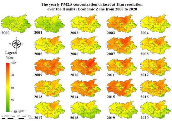
3.2. Yearly PM2.5 Concentration Dataset

With the modeled daily PM2.5 concentration, we calculated the modeled monthly and seasonal PM2.5 concentration, averaged from 2000 to 2020 (Figure A1) and produced the yearly PM2.5 concentration dataset by averaging the modeled daily PM2.5 concentration (Figure A2). As described in Section 2.3.3, we performed a quality assessment on the synthesized yearly PM2.5 concentration dataset. The number of available sites, time range, number of available data items (hourly data per day), and missing-data rate from 2015–2020 are shown in Table 3.
The year-specific data quality assessment result is shown in Figure 6, with R 2   ranging from 0.69 to 0.79 (Figure 6a–f). The overall data quality assessment result from 2015 to 2020 shows that R 2 = 0.77, R M S E = 6.92 μg/m³, and M A E = 5.42 μg/m³ (Figure 6g). This shows that the synthesized yearly PM2.5 concentration dataset is reliable and can be used for further analysis. In addition, we also validated the modeled monthly PM2.5 by comparing it with the observed monthly PM2.5 data from available monitoring sites between 2015 and 2020 (Figure A3).

3.3. Trend Analysis

The yearly average PM2.5 concentration of the entire study area from 2000 to 2020 was calculated and plotted in Figure 7. This figure shows that the yearly average PM2.5 of the zone increased and then decreased with time, with the highest value being in 2010. After testing for linear, exponential, logarithmic, polynomial, and multiplicative power fit, we selected the polynomial fit as the best method by comparing values of R². It is found that a quadratic model was the best fit for the data, with R 2 = 0.63 and the highest point of the curve falling in the year of 2010. This means that the 21-year period could be divided into two stages: the one from 2000–2010 as the upward stage and the other from 2010–2020 as the downward stage.
As described in Section 2.3.4, the Theil-Sen slopes of yearly PM2.5 concentration over the Huaihai Economic Zone from 2000–2010, 2010–2020, and 2000–2020 were calculated to reveal the change on a pixel scale. The Mann-Kendall trend test was then performed on the calculated Theil-Sen slope maps to calculate the significance of the changes. Figure 8 shows the Theil-Sen slope maps and Mann-Kendall trend test results of the yearly PM2.5 concentration for the 2000–2010 and 2010–2020 stages and the entire 2000–2020 period, respectively. As the majority of the slope values ranged from −2 to 2 and there is a need to discriminate positive and negative values, the resultant slope maps were classified into six levels, with the range from −2 to 2 divided into four levels with increments of 1.
The combined results of the Theil-Sen estimator and the Mann-Kendall trend test show that during the 2000–2010 stage, 91.5% of the study area saw a significantly increasing trend in PM2.5 concentration, and most of the slope values were within the range of 1–2 (Figure 8b). From 2010 to 2020, 69.59% of the study area had a significantly decreasing trend in PM2.5 concentration, mostly in the west and south of the Zone (Figure 8d). For the entire period from 2000 to 2020, however, only 1% of the study area passed the significance test (Figure 8f), mainly in the Nansi Lake area at the junction of the Shandong and Jiangsu provinces (Figure 8g) and the Hongze Lake area at the southeast corner of the Zone (Figure 8h).

4. Discussion

4.1. Random Forest Modeling

PM2.5 concentration can be estimated from AOD based on their close correlation [13,71] but the inclusion of additional variables can improve the estimation [72,73]. In this study, we considered factors such as meteorology, topography, date, and location. The correlation analysis result (Table 1) proves that these variables are significantly correlated with PM2.5, except for total precipitation. Date and location represent the spatiotemporal heterogeneity of PM2.5 concentration. Latitude and longitude were used by Yang and Huang as variables for land cover classification using random forest [74]. In this study, we also examined the effect of the two variables by removing them from modeling. The results show that R 2 decreased to 0.849 with the exclusion of latitude and longitude, which is lower than the value of 0.853 from when these variables were included (Figure 5). This has further proved that the two variables play a role in the random forest model.
In addition to AOD, T2M and date have high correlations with PM2.5 and high feature importance, which means that the two variables are essential for PM2.5 concentration modeling. The role of T2M can be explained by the fact that five cities (Xuzhou, Linyi, Zaozhuang, Jining, and Heze) in the Zone have central heating systems used in the cold months, so there are more PM2.5 emissions when temperatures are low [75]. It is noted that date has a low correlation with PM2.5 but that its feature importance was the highest in the random forest model. Pearson correlations capture the linear relationship between different variables, but feature importance in random forest identifies the level of influence of features for classification or regression. A low correlation coefficient only means a lower linear correlation but does not necessarily imply lower feature importance in the random forest regression. The high feature importance of date means that it plays a very important role in the regression process. As previous studies have shown [75,76,77], PM2.5 concentration does not simply increase or decrease over time, but is high over some periods (October to February) and low over others (March to September) within the same year. Admittedly, features with higher importance are considered more important than those with lower importance [51,78]; however, explaining differences in feature importance is not straightforward as feature importance might not be physically meaningful [51].
In addition to the ranking of features’ importance, the main advantage of random forest regression lies in improved accuracy. Based on the ensemble learning technique, random forest creates many trees on the subset of data and combines all the trees’ outputs. In this way, it reduces overfitting and is therefore more capable of prediction than other models. The R 2 was 0.84 on the validation data and 0.85 on the testing data (Section 3.1), which suggests that overfitting was not an issue here and that the resultant random forest model was robust. In terms of accuracy, our model (Figure 4) ( R ² = 0.85, R M S E = 14.63 μg/m³) outperforms the model obtained by Wei et al. ( R ² = 0.85, R M S E = 15.57 μg/m³) [25] that estimated 1-km PM2.5 concentrations across China using the same source of AOD data and a random forest method. Our accuracy is much higher than that of Guo et al. [26] where various data were used to estimate 1-km PM2.5 concentrations across China without considering their spatial and temporal variability.

4.2. Yearly PM2.5 Concentration Dataset

With the validated daily PM2.5 concentration model, daily PM2.5 concentration over the Huaihai Economic Zone at a 1 km resolution could be estimated from 2000 to 2020. Subsequently, it was possible to produce a monthly, seasonal, or yearly PM2.5 concentration dataset at a resolution of 1 km by averaging the modeled daily PM2.5 concentrations over the study area for further analysis and applications. Monthly, seasonal, and yearly PM2.5 concentration datasets would contribute to the examination of the monthly, seasonal, and yearly variabilities of PM2.5 concentration. As it is most interesting to examine the trends of PM2.5 concentration during the last two decades, this study focuses on the production of the yearly PM2.5 concentration dataset. To our knowledge, the PM2.5 pollution over the Huaihai Economic Zone is less studied, although it has a history of poor air quality and is located between two large polluted urban agglomerations (i.e., the Beijing-Tianjin-Hebei Region and the Yangtze River Delta). This study provides a feasible way to produce yearly PM2.5 concentration datasets for air quality monitoring.
A good daily PM2.5 concentration estimation model can produce good daily PM2.5 concertation data, but this does not necessarily guarantee a reliable yearly dataset because there is missing AOD data for some days. However, the quality assessment shows that the accuracy of the yearly PM2.5 concentration dataset is good ( R ² = 0.77, R M S E = 6.92 μg/m³, and M A E = 5.42 μg/m³) (Figure 6g), which suggests that missing AOD data are not causing issues in our study. However, we believe that if there were more days with recorded AOD data, there would be more modeled daily PM2.5 data and the already high quality of the yearly dataset could have been further improved. The synthesized yearly dataset can serve as a ready-for-use source of data for multiple purposes, such as the analysis of the relationship between population exposure and diseases [79,80], the identification of the drivers of PM2.5 emissions [81,82], and the trend analysis of PM2.5 concentration, as demonstrated in this study.

4.3. Trend Analysis

Both the scatterplot of the yearly average PM2.5 (Figure 6) and the Theil-Sen estimator’s result (Figure 8a,c,e) clearly show that PM2.5 concentration had an upward trend from 2000–2010 and a downward trend from 2010–2020. This finding is similar to that of Wang et al. [67] who examined the spatiotemporal variability of PM2.5 concentration in China. Although the Theil-Sen estimator’s result illustrates that nearly the entire zone had changes during the three periods, only part of the zone experienced significant increases or decreased in PM2.5 concentration (Figure 8b,d,f).
In the 2000–2010 stage, there was a significant, increasing trend in the Zone, especially for the four cities of Shandong (Linyi, Zaozhuang, Jining and Heze) and the two cities of Anhui (Suzhou and Huaibei) (Figure 8b), for which most of the slope values were >1. There are multiple reasons for this finding. Firstly, the Shandong province has the highest air pollutant emissions in China due to heavy coal consumption in the electrical power sector and the high concentration of coal-fired power plants [83]. Its PM2.5 concentration increases from east to west, and the western part of Shandong is heavily polluted [84], including the four Shandong cities of the Zone. Secondly, the northeastern part of the Zone is in the Yimeng Mountain area (the high-elevation areas in Figure 1b), which is not conducive to the diffusion of pollutants and therefore results in serious local air pollution [85]. Lastly, air pollution from polluted neighboring regions, such as the Beijing-Tianjin-Hebei region and the Yangtze River Delta region should be not ignored. Shi et al. reported that pollution in Anhui was originally from the Yangtze River Delta region and particularly intense in the two Anhui cities of the Zone [86].
The trend of PM2.5 concentration changed to be completely different from the increasing in the 2000–2010 stage to the decreasing in the 2010–2020 stage. We believe that this is attributed to China’s air pollution countermeasures. In 2012, China released a new ambient air quality standard (GB 2095-2012), setting limits on the levels of PM2.5 for the first time [87]. Although it only took effect nationwide in 2016, many cities and regions in China were required to implement the new standard earlier. China set up a national air quality monitoring network in 2012, initially comprising of 496 monitoring sites in 74 cities [88] (including Xuzhou and Lianyungang), which is now extended to 956 monitoring sites in 190 cities [11]. The network allows cities to monitor and release readings on PM2.5 and many other pollutants. In the same year, China also issued the Air Pollution Prevention and Control Action Plan to mitigate air pollution and its associated health impacts [89]. Comprising of 10 specific measures, this action was considered as the most stringent air pollution control policy in China. In addition to the national policies, provinces and cities also issued their own, respective plans. Data show that the investment in environmental protection in the provinces of Jiangsu, Shandong, Henan, and Anhui increased significantly from 2010 to 2020 [90,91,92,93]. All these initiatives have, together, contributed to the improvement of air quality in the zone in recent years.
Despite a significant increasing trend in the 2000–2010 stage and a significant decreasing trend in the 2010–2020 stage, the overall trend of PM2.5 concentration over the Huaihai Economic Zone remained decreasing during the 21 years (Figure 8f). It appears that the improvement in the second stage offset the deterioration in the first stage. However, the area of the significantly increasing trend was much smaller and mainly distributed in the Nansi Lake area (Figure 8g) and surrounding the Hongze Lake area (Figure 8h). This finding suggests that although air quality has been considerably improved in the wetlands, there is a need for continuous and more intensive efforts to decrease the overall PM2.5 concentration in the Zone.

4.4. Innovations and Limitations

The innovation of the study is making use of the added values of random forest to model daily PM2.5 concentration. In addition, in the modeling process, extra variables, such as date and location, were included as these variables represent the spatiotemporal heterogeneity of PM2.5 concentration and therefore serve to improve the model’s accuracy. However, there are also some limitations to the study, which need to be addressed in future work. The spatial coverage of the MAIAC AOD data used in this study is generally not very high, such that PM2.5 was not modeled for every pixel in the Zone. Sample data for training are mainly concentrated in the spring and winter due to the availability of AOD data, which may lead to less accurate PM2.5 predictions in the summer and autumn. If the spatial resolution of meteorological data was higher, PM2.5 concentration maps would have been more evenly distributed.
In addition, our study only estimates regional PM2.5 concentration and it is unclear how well our model would perform when applied at a larger scale. It would be interesting to test the model and, if necessary, improve it for estimating PM2.5 concentrations over the entire mainland of China and compare our results with other studies.

5. Conclusions

In order to better estimate the 1-km resolution, daily PM2.5 concentration from the MAIAC AOD dataset, this study considers additional variables and uses random forest regression to construct a daily PM2.5 concentration estimation model using the case study of the Huaihai Economic Zone from 2000 to 2020. From the results, it is concluded that:
  • Random forest is capable of modeling daily PM2.5 concentration over a large geographic area with an accuracy of R 2 = 0.85. In addition to AOD, date is an important feature that should be considered.
  • A yearly PM2.5 concentration dataset at a 1 km resolution can be synthesized by averaging modeled daily PM2.5 concentration data. It has a data quality of R 2 = 0.77 and can be considered a ready-for-use dataset for various purposes.
  • Although increasing from 2000–2010 and decreasing from 2010–2020, the trend of PM2.5 concentration was significantly decreasing overall over the last two decades. The area of the significantly increasing trend was small and mainly distributed in the lake areas in the zone.
This study contributes to a better understanding of the influencing factors of PM2.5 pollution and demonstrates the potential of random forest for modeling PM2.5 concentrations. It also examines the changes of PM2.5 levels over time and justifies the necessity of adopting context-specific PM2.5 prevention measures by decision-makers and environmental managers.

Author Contributions

Conceptualization, X.L. and L.L.; methodology, X.L. and L.L.; software, X.L.; validation, X.L. and L.L.; formal analysis, X.L. and L.L.; investigation, X.L. and L.L.; resources, L.L., L.C. (Longgao Chen) and L.C. (Longqian Chen); data curation, X.L., T.Z. and J.X.; writing—original draft preparation, X.L. and L.L.; writing—review and editing, L.L., L.C. (Longgao Chen) and L.C. (Longqian Chen); visualization, X.L., L.C. (Longgao Chen), T.Z. and J.X.; supervision, L.L.; project administration, L.L. and L.C. (Longqian Chen); funding acquisition, L.L. All authors have read and agreed to the published version of the manuscript.

Funding

This research was funded by the National Natural Science Foundation of China (Grant No. 42001212). It was also supported by the Research Center for Transition Development and Rural Revitalization of Resource-Based Cities in China, China University of Mining and Technology.

Institutional Review Board Statement

Not applicable.

Informed Consent Statement

Not applicable.

Data Availability Statement

Data can be obtained by a personal request to the first author.

Acknowledgments

The authors would like to thank Earthdata for providing the MAIAC AOD data, the Climate Change Service (CDS) for providing the ERA5-Land hourly data, the Geospatial Data Cloud for providing the digital elevation model (DEM) dataset, and the China National Environmental Monitoring Centre for providing the PM2.5 ground observing data. We appreciate the editors and reviewers for their constructive comments and suggestions for improving the overall quality of the study.

Conflicts of Interest

The authors declare no conflict of interest.

Appendix A

With the determined random forest model (Section 3.1), we modeled the daily PM2.5 concentration at a 1 km resolution over the Huaihai Economic Zone from 2000 to 2020. Subsequently, we calculated the modeled monthly and seasonal PM2.5 concentrations, averaged from 2000 to 2020 (Figure A1) and produced the 1 km-resolution, yearly PM2.5 concentration dataset by averaging the modeled daily PM2.5 concentration (Figure A2).
Figure A1. The modeled monthly and seasonal PM2.5 concentrations, averaged from 2000 to 2020. The modeled monthly PM2.5 concentrations for the study area (a) were obtained by averaging the modeled daily PM2.5 concentration in the same months from 2000 to 2020. Similarly, we calculated the modeled seasonal PM2.5 concentration from 2000 to 2020 (b). PM2.5 concentration decreased and then increased with month and season. In addition, PM2.5 concentrations in cold months were higher than in warm months.
Sustainability 14 08520 g0a1
Figure A2. The yearly PM2.5 concentration dataset at a 1 km resolution over the Huaihai Economic Zone from 2000 to 2020.
Sustainability 14 08520 g0a2
Figure A3. Data quality assessment by comparing the values for the modeled monthly PM2.5 concentration with the observed monthly PM2.5 concentration from available monitoring sites in the years from 2015 to 2020.
Sustainability 14 08520 g0a3

References

  1. Dominski, F.H.; Branco, J.H.L.; Buonanno, G.; Stabile, L.; da Silva, M.G.; Andrade, A. Effects of air pollution on health: A mapping review of systematic reviews and meta-analyses. Environ. Res. 2021, 201, 111487. [Google Scholar] [CrossRef] [PubMed]
  2. World Health Organization. WHO Issues Latest Global Air Quality Report: Some Progress, but More Attention Needed to Avoid Dangerously High Levels of Air Pollution. Available online: https://www.who.int/china/news/detail/02-05-2018-who-issues-latest-global-air-quality-report-some-progress-but-more-attention-needed-to-avoid-dangerously-high-levels-of-air-pollution (accessed on 22 April 2022).
  3. World Health Organization. Billions of People Still Breathe Unhealthy Air: New WHO Data. Available online: https://www.who.int/news/item/04-04-2022-billions-of-people-still-breathe-unhealthy-air-new-who-data (accessed on 22 April 2022).
  4. State of Globe Air. Global Health Impacts of Air Pollution. Available online: https://www.stateofglobalair.org/health/global#Millions-deaths (accessed on 20 April 2022).
  5. Ministry of Ecology of Environment of the People’s Republic of China. China Ecological and Environmental Status Bulletin 2020. Available online: https://www.mee.gov.cn/hjzl/sthjzk/zghjzkgb/202105/P020210526572756184785.pdf (accessed on 20 April 2022).
  6. Li, J.; Chen, L.; Xiang, Y.; Xu, M. Research on Influential Factors of PM2.5 within the Beijing-Tianjin-Hebei Region in China. Discret. Dyn. Nat. Soc. 2018, 2018, 6375391. [Google Scholar] [CrossRef] [Green Version]
  7. Zhang, X.; Shi, M.; Li, Y.; Pang, R.; Xiang, N. Correlating PM2.5 concentrations with air pollutant emissions: A longitudinal study of the Beijing-Tianjin-Hebei region. J. Clean. Prod. 2018, 179, 103–113. [Google Scholar] [CrossRef]
  8. Su, Z.; Lin, L.; Chen, Y.; Hu, H. Understanding the distribution and drivers of PM2.5 concentrations in the Yangtze River Delta from 2015 to 2020 using Random Forest Regression. Environ. Monit. Assess. 2022, 194, 284. [Google Scholar] [CrossRef]
  9. Wang, M.; Wang, H. Spatial Distribution Patterns and Influencing Factors of PM2.5 Pollution in the Yangtze River Delta: Empirical Analysis Based on a GWR Model. Asia-Pac. J. Atmos. Sci. 2021, 57, 63–75. [Google Scholar] [CrossRef]
  10. Greennet Environment Protection. National air Quality Ranking and Analysis in 2020. Available online: https://mp.weixin.qq.com/s/MQp6cKdCqcSaH3em0tnmaA (accessed on 20 April 2022).
  11. Zhang, Y.-L.; Cao, F. Fine particulate matter (PM2.5) in China at a city level. Sci. Rep. 2015, 5, 14884. [Google Scholar] [CrossRef] [Green Version]
  12. Liu, Y.; Paciorek, C.J.; Koutrakis, P. Estimating regional spatial and temporal variability of PM2.5 concentrations using satellite data, meteorology, and land use information. Environ. Health Perspect. 2009, 117, 886–892. [Google Scholar] [CrossRef] [Green Version]
  13. Yang, Q.; Yuan, Q.; Yue, L.; Li, T.; Shen, H.; Zhang, L. The relationships between PM2.5 and aerosol optical depth (AOD) in mainland China: About and behind the spatio-temporal variations. Environ. Pollut. 2019, 248, 526–535. [Google Scholar] [CrossRef]
  14. Lin, C.Q.; Li, Y.; Yuan, Z.B.; Lau, A.K.H.; Li, C.C.; Fung, J.C.H. Using satellite remote sensing data to estimate the high-resolution distribution of ground-level PM2.5. Remote Sens. Environ. 2015, 156, 117–128. [Google Scholar] [CrossRef]
  15. He, Q.Q.; Gu, Y.F.; Zhang, M. Spatiotemporal trends of PM2.5 concentrations in central China from 2003 to 2018 based on MAIAC-derived high-resolution data. Environ. Int. 2020, 137, 105536. [Google Scholar] [CrossRef]
  16. Xu, X.; Zhang, C.; Liang, Y. Review of satellite-driven statistical models PM2.5 concentration estimation with comprehensive information. Atmos. Environ. 2021, 256, 118302. [Google Scholar] [CrossRef]
  17. Lu, J.; Zhang, Y.H.; Chen, M.X.; Wang, L.; Zhao, S.H.; Pu, X.; Chen, X.G. Estimation of monthly 1 km resolution PM2.5 concentrations using a random forest model over “2 + 26” cities, China. Urban Clim. 2021, 35, 100734. [Google Scholar] [CrossRef]
  18. Masini, R.P.; Medeiros, M.C.; Mendes, E.F. Machine Learning Advances for Time Series Forecasting. J. Econ. Surv. 2021, 36. in press. [Google Scholar] [CrossRef]
  19. Wu, D.J.; Zewdie, G.K.; Liu, X.; Kneen, M.A.; Lary, D.J. Insights into the Morphology of the East Asia PM2.5 Annual Cycle Provided by Machine Learning. Environ. Health Insights 2017, 11, 7. [Google Scholar] [CrossRef] [PubMed] [Green Version]
  20. Mhawish, A.; Banerjee, T.; Sorek-Hamer, M.; Bilal, M.; Lyapustin, A.I.; Chatfield, R.; Broday, D.M. Estimation of High-Resolution PM2.5 over the Indo-Gangetic Plain by Fusion of Satellite Data, Meteorology, and Land Use Variables. Environ. Sci. Technol. 2020, 54, 7891–7900. [Google Scholar] [CrossRef]
  21. Choubin, B.; Abdolshahnejad, M.; Moradi, E.; Querol, X.; Mosavi, A.; Shamshirband, S.; Ghamisi, P. Spatial hazard assessment of the PM10 using machine learning models in Barcelona, Spain. Sci. Total Environ. 2020, 701, 134474. [Google Scholar] [CrossRef]
  22. Han, S.; Yang, X.; Zhou, Q.; Zhuang, J.; Wu, W. Predicting biomarkers from classifier for liver metastasis of colorectal adenocarcinomas using machine learning models. Cancer Med. 2020, 9, 6667–6678. [Google Scholar] [CrossRef]
  23. Jamthikar, A.; Gupta, D.; Khanna, N.N.; Saba, L.; Araki, T.; Viskovic, K.; Suri, H.S.; Gupta, A.; Mavrogeni, S.; Turk, M.; et al. A low-cost machine learning-based cardiovascular/stroke risk assessment system: Integration of conventional factors with image phenotypes. Cardiovasc. Diagn. Ther. 2019, 9, 420–430. [Google Scholar] [CrossRef] [Green Version]
  24. Wang, Z.L.; Lai, C.G.; Chen, X.H.; Yang, B.; Zhao, S.W.; Bai, X.Y. Flood hazard risk assessment model based on random forest. J. Hydrol. 2015, 527, 1130–1141. [Google Scholar] [CrossRef]
  25. Wei, J.; Huang, W.; Li, Z.Q.; Xue, W.H.; Peng, Y.R.; Sun, L.; Cribb, M. Estimating 1-km-resolution PM2.5 concentrations across China using the space-time random forest approach. Remote Sens. Environ. 2019, 231, 111221. [Google Scholar] [CrossRef]
  26. Guo, B.; Zhang, D.; Pei, L.; Su, Y.; Wang, X.; Bian, Y.; Zhang, D.; Yao, W.; Zhou, Z.; Guo, L. Estimating PM2.5 concentrations via random forest method using satellite, auxiliary, and ground-level station dataset at multiple temporal scales across China in 2017. Sci. Total Environ. 2021, 778, 146288. [Google Scholar] [CrossRef] [PubMed]
  27. Shogrkhodaei, S.Z.; Razavi-Termeh, S.V.; Fathnia, A. Spatio-temporal modeling of PM2.5 risk mapping using three machine learning algorithms. Environ. Pollut. 2021, 289, 117859. [Google Scholar] [CrossRef] [PubMed]
  28. Stafoggia, M.; Bellander, T.; Bucci, S.; Davoli, M.; de Hoogh, K.; de’Donato, F.; Gariazzo, C.; Lyapustin, A.; Michelozzi, P.; Renzi, M.; et al. Estimation of daily PM10 and PM2.5 concentrations in Italy, 2013-2015, using a spatiotemporal land-use random-forest model. Environ. Int. 2019, 124, 170–179. [Google Scholar] [CrossRef]
  29. Hu, X.F.; Belle, J.H.; Meng, X.; Wildani, A.; Waller, L.A.; Strickland, M.J.; Liu, Y. Estimating PM2.5 Concentrations in the Conterminous United States Using the Random Forest Approach. Environ. Sci. Technol. 2017, 51, 6936–6944. [Google Scholar] [CrossRef] [PubMed]
  30. Yazdi, M.D.; Kuang, Z.; Dimakopoulou, K.; Barratt, B.; Suel, E.; Amini, H.; Lyapustin, A.; Katsouyanni, K.; Schwartz, J. Predicting Fine Particulate Matter (PM2.5) in the Greater London Area: An Ensemble Approach using Machine Learning Methods. Remote Sens. 2020, 12, 914. [Google Scholar] [CrossRef] [Green Version]
  31. Ghahremanloo, M.; Choi, Y.; Sayeed, A.; Salman, A.K.; Pan, S.; Amani, M. Estimating daily high-resolution PM2.5 concentrations over Texas: Machine Learning approach. Atmos. Environ. 2021, 247, 118209. [Google Scholar] [CrossRef]
  32. Tian, H.; Zhao, Y.; Luo, M.; He, Q.; Han, Y.; Zeng, Z. Estimating PM2.5 from multisource data: A comparison of different machine learning models in the Pearl River Delta of China. Urban Clim. 2021, 35, 100740. [Google Scholar] [CrossRef]
  33. Ma, Z.W.; Hu, X.F.; Sayer, A.M.; Levy, R.; Zhang, Q.; Xue, Y.G.; Tong, S.L.; Bi, J.; Huang, L.; Liu, Y. Satellite-based spatiotemporal trends in PM2.5 Concentrations: China, 2004–2013. Environ. Health Perspect. 2016, 124, 184–192. [Google Scholar] [CrossRef] [Green Version]
  34. Yang, W.T.; Deng, M.; Xu, F.; Wang, H. Prediction of hourly PM2.5 using a space-time support vector regression model. Atmos. Environ. 2018, 181, 12–19. [Google Scholar] [CrossRef]
  35. Connell, D.P.; Withum, J.A.; Winter, S.E.; Statnick, R.M.; Bilonick, R.A. The Steubenville Comprehensive Air Monitoring Program (SCAMP): Overview and statistical considerations. J. Air Waste Manag. Assoc. 2005, 55, 467–480. [Google Scholar] [CrossRef] [Green Version]
  36. State Council of the People’s Republic of China. The Approval of the State Council on the Overall Urban Planning of Xuzhou. Available online: http://www.gov.cn/zhengce/content/2017-06/23/content_5204776.htm (accessed on 19 April 2022).
  37. National Development and Reform Commission. Notice of the National Development and Reform Commission concerning Printing and Distributing the Huaihe Ecological Ecomnmic Belt Development Plan. Available online: https://www.ndrc.gov.cn/xxgk/zcfb/ghwb/201811/t20181107_962252.html?code=&state=123 (accessed on 20 April 2022).
  38. Lyapustin, A. Description of MCD19A2 v006. Available online: https://lpdaac.usgs.gov/products/mcd19a2v006/ (accessed on 26 April 2022).
  39. Cheng, L.; Li, L.; Chen, L.; Hu, S.; Yuan, L.; Liu, Y.; Cui, Y.; Zhang, T. Spatiotemporal Variability and Influencing Factors of Aerosol Optical Depth over the Pan Yangtze River Delta during the 2014–2017 Period. Int. J. Environ. Res. Public Health 2019, 16, 3522. [Google Scholar] [CrossRef] [PubMed] [Green Version]
  40. Bai, Y.; Wu, L.; Qin, K.; Zhang, Y.; Shen, Y.; Zhou, Y. A Geographically and Temporally Weighted Regression Model for Ground-Level PM2.5 Estimation from Satellite-Derived 500 m Resolution AOD. Remote Sens. 2016, 8, 262. [Google Scholar] [CrossRef] [Green Version]
  41. Ni, X.; Cao, C.; Zhou, Y.; Cui, X.; Singh, R.P. Spatio-Temporal Pattern Estimation of PM2.5 in Beijing-Tianjin-Hebei Region Based on MODIS AOD and Meteorological Data Using the Back Propagation Neural Network. Atmosphere 2018, 9, 105. [Google Scholar] [CrossRef] [Green Version]
  42. Cheng, L. Research on Remote Sensing Estimation of PM 2.5 Concentration and Its Interaction with Urbanization in the Yangtze River Delta; China University of Mining and Technology: Xuzhou, China, 2021. [Google Scholar] [CrossRef]
  43. European Centre for Medium-Range Weather Forecasts. ECMWF Reanalysis v5—Land (ERA5-LAND). Available online: https://www.ecmwf.int/en/forecasts/dataset/ecmwf-reanalysis-v5-land (accessed on 22 April 2022).
  44. European Centre for Medium-Range Weather Forecasts. CDS Dataset Documentation of ERA5. Available online: https://confluence.ecmwf.int/display/CKB/ERA5 (accessed on 23 April 2022).
  45. Jing, Z.; Liu, P.; Wang, T.; Song, H.; Lee, J.; Xu, T.; Xing, Y. Effects of Meteorological Factors and Anthropogenic Precursors on PM2.5 Concentrations in Cities in China. Sustainability 2020, 12, 3550. [Google Scholar] [CrossRef]
  46. Zang, Z.; Wang, W.; Cheng, X.; Yang, B.; Pan, X.; You, W. Effects of Boundary Layer Height on the Model of Ground-Level PM2.5 Concentrations from AOD: Comparison of Stable and Convective Boundary Layer Heights from Different Methods. Atmosphere 2017, 8, 104. [Google Scholar] [CrossRef] [Green Version]
  47. Lou, M.Y.; Guo, J.P.; Wang, L.L.; Xu, H.; Chen, D.D.; Miao, Y.C.; Lv, Y.M.; Li, Y.; Guo, X.R.; Ma, S.L.; et al. On the Relationship Between Aerosol and Boundary Layer Height in Summer in China Under Different Thermodynamic Conditions. Earth Space Sci. 2019, 6, 887–901. [Google Scholar] [CrossRef] [Green Version]
  48. Jin, X.; Cai, X.; Yu, M.; Song, Y.; Wang, X.; Kang, L.; Zhang, H. Diagnostic analysis of wintertime PM2.5 pollution in the North China Plain: The impacts of regional transport and atmospheric boundary layer variation. Atmos. Environ. 2020, 224, 117346. [Google Scholar] [CrossRef]
  49. Zhang, L.; Guo, X.; Zhao, T.; Gong, S.; Xu, X.; Li, Y.; Luo, L.; Gui, K.; Wang, H.; Zheng, Y.; et al. A modelling study of the terrain effects on haze pollution in the Sichuan Basin. Atmos. Environ. 2019, 196, 77–85. [Google Scholar] [CrossRef]
  50. Breiman, L. Random Forests. Mach. Learn. 2001, 45, 5–32. [Google Scholar] [CrossRef] [Green Version]
  51. Li, L.; Solana, C.; Canters, F.; Kervyn, M. Testing random forest classification for identifying lava flows and mapping age groups on a single Landsat 8 image. J. Volcanol. Geotherm. Res. 2017, 345, 109–124. [Google Scholar] [CrossRef] [Green Version]
  52. Rodriguez-Galiano, V.; Sanchez-Castillo, M.; Chica-Olmo, M.; Chica-Rivas, M. Machine learning predictive models for mineral prospectivity: An evaluation of neural networks, random forest, regression trees and support vector machines. Ore Geol. Rev. 2015, 71, 804–818. [Google Scholar] [CrossRef]
  53. Goetz, J.N.; Brenning, A.; Petschko, H.; Leopold, P. Evaluating machine learning and statistical prediction techniques for landslide susceptibility modeling. Comput. Geosci. 2015, 81, 1–11. [Google Scholar] [CrossRef]
  54. Boulesteix, A.L.; Janitza, S.; Kruppa, J.; Konig, I.R. Overview of random forest methodology and practical guidance with emphasis on computational biology and bioinformatics. Wiley Interdiscip. Rev. Data Min. Knowl. Discov. 2012, 2, 493–507. [Google Scholar] [CrossRef] [Green Version]
  55. Liaw, A.; Wiener, M. Classification and regression by randomforest. Forest 2001, 2, 18–22. [Google Scholar]
  56. Scikit Learn. Random Forest Regressor. Available online: https://scikit-learn.org/stable/modules/generated/sklearn.ensemble.RandomForestRegressor.html (accessed on 22 April 2022).
  57. Arlot, S.; Celisse, A. A survey of cross-validation procedures for model selection. Statist. Surv. 2010, 4, 40–79. [Google Scholar] [CrossRef]
  58. Liu, H.; Cocea, M. Semi-random partitioning of data into training and test sets in granular computing context. Granul. Comput. 2017, 2, 357–386. [Google Scholar] [CrossRef] [Green Version]
  59. Bui, D.T.; Pradhan, B.; Lofman, O.; Revhaug, I. Landslide Susceptibility Assessment in Vietnam Using Support Vector Machines, Decision Tree, and Naive Bayes Models. Math. Probl. Eng. 2012, 2012, 974638. [Google Scholar] [CrossRef] [Green Version]
  60. Vrigazova, B. The Proportion for Splitting Data into Training and Test Set for the Bootstrap in Classification Problems. Bus. Syst. Res. J. 2021, 12, 228–242. [Google Scholar] [CrossRef]
  61. Jung, Y. Multiple predicting K-fold cross-validation for model selection. J. Nonparametr. Stat. 2018, 30, 197–215. [Google Scholar] [CrossRef]
  62. Radhakrishna, R.C.; Shalabh; Helge, T.; Christian, H. Linear Models and Generalizations, 3rd ed.; Springer: Berlin/Heidelberg, Germany, 2008. [Google Scholar]
  63. Li, L.; Bakelants, L.; Solana, C.; Canters, F.; Kervyn, M. Dating lava flows of tropical volcanoes by means of spatial modeling of vegetation recovery. Earth Surf. Process. Landf. 2018, 43, 840–856. [Google Scholar] [CrossRef]
  64. Li, L.; Zhou, X.S.; Chen, L.Q.; Chen, L.G.; Zhang, Y.; Liu, Y.Q. Estimating Urban Vegetation Biomass from Sentinel-2A Image Data. Forests 2020, 11, 24. [Google Scholar] [CrossRef] [Green Version]
  65. Gocic, M.; Trajkovic, S. Analysis of changes in meteorological variables using Mann-Kendall and Sen’s slope estimator statistical tests in Serbia. Glob. Planet. Change 2013, 100, 172–182. [Google Scholar] [CrossRef]
  66. Sen, P.K. Estimates of the Regression Coefficient Based on Kendall’s Tau. J. Am. Stat. Assoc. 1968, 63, 1379–1389. [Google Scholar] [CrossRef]
  67. Wang, X.; Li, T.; Ikhumhen, H.O.; Sá, R.M. Spatio-temporal variability and persistence of PM2.5 concentrations in China using trend analysis methods and Hurst exponent. Atmos. Pollut. Res. 2022, 13, 101274. [Google Scholar] [CrossRef]
  68. Mann, H.B. Nonparametric Tests Against Trend. Econometrica 1945, 13, 245–259. [Google Scholar] [CrossRef]
  69. Kendall, M.G. Rank Correlation Methods; Griffin: London, UK, 1975. [Google Scholar]
  70. Wang, F.; Shao, W.; Yu, H.; Kan, G.; He, X.; Zhang, D.; Ren, M.; Wang, G. Re-evaluation of the Power of the Mann-Kendall Test for Detecting Monotonic Trends in Hydrometeorological Time Series. Front. Earth Sci. 2020, 8, 14. [Google Scholar] [CrossRef]
  71. Ma, Z.; Hu, X.; Huang, L.; Bi, J.; Liu, Y. Estimating Ground-Level PM2.5 in China Using Satellite Remote Sensing. Environ. Sci. Technol. 2014, 48, 7436–7444. [Google Scholar] [CrossRef]
  72. Di, Q.; Amini, H.; Shi, L.; Kloog, I.; Silvern, R.; Kelly, J.; Sabath, M.B.; Choirat, C.; Koutrakis, P.; Lyapustin, A.; et al. An ensemble-based model of PM2.5 concentration across the contiguous United States with high spatiotemporal resolution. Environ. Int. 2019, 130, 104909. [Google Scholar] [CrossRef]
  73. Sun, J.; Gong, J.; Zhou, J. Estimating hourly PM2.5 concentrations in Beijing with satellite aerosol optical depth and a random forest approach. Sci. Total Environ. 2021, 762, 144502. [Google Scholar] [CrossRef] [PubMed]
  74. Yang, J.; Huang, X. The 30 m annual land cover dataset and its dynamics in China from 1990 to 2019. Earth Syst. Sci. Data 2021, 13, 3907–3925. [Google Scholar] [CrossRef]
  75. Wu, X.G.; Ding, Y.Y.; Zhou, S.B.; Tan, Y. Temporal characteristic and source analysis of PM2.5 in the most polluted city agglomeration of China. Atmos. Pollut. Res. 2018, 9, 1221–1230. [Google Scholar] [CrossRef]
  76. Gao, S.L.; Yang, L.; Dong, S.Z.; Sun, W.; Zha, K.C.; Zhao, J.D. A Study on Spatial-temporal Distribution Characteristics of PM2.5 Concentrations in Nanjing during 2012–2016. In Proceedings of the 2nd International Conference on Materials Science, Energy Technology and Environmental Engineering (MSETEE), Zhuhai, China, 28–30 April 2017. [Google Scholar] [CrossRef]
  77. Wang, Z.-B.; Fang, C.-L. Spatial-temporal characteristics and determinants of PM2.5 in the Bohai Rim Urban Agglomeration. Chemosphere 2016, 148, 148–162. [Google Scholar] [CrossRef] [PubMed]
  78. Aldrich, C.; Auret, L. Fault detection and diagnosis with random forest feature extraction and variable importance methods. IFAC Proc. Vol. 2010, 43, 79–86. [Google Scholar] [CrossRef]
  79. Leonardi, G.S.; Houthuijs, D.; Steerenberg, P.A.; Fletcher, T.; Armstrong, B.; Antova, T.; Lochman, I.; Lochmanova, A.; Rudnai, P.; Erdei, E.; et al. Immune biomarkers in relation to exposure to particulate matter: A cross-sectional survey in 17 cities of central Europe. Inhal. Toxicol. 2000, 12, 1–14. [Google Scholar] [CrossRef]
  80. Badyda, A.J.; Grellier, J.; Dabrowiecki, P. Ambient PM2.5 Exposure and Mortality Due to Lung Cancer and Cardiopulmonary Diseases in Polish Cities. In Respiratory Treatment and Prevention; Pokorski, M., Ed.; Springer: Berlin/Heidelberg, Germany, 2017; Volume 944, pp. 9–17. [Google Scholar] [CrossRef]
  81. Lang, J.; Cheng, S.; Li, J.; Chen, D.; Zhou, Y.; Wei, X.; Han, L.; Wang, H. A Monitoring and Modeling Study to Investigate Regional Transport and Characteristics of PM2.5 Pollution. Aerosol Air Qual. Res. 2013, 13, 943–956. [Google Scholar] [CrossRef] [Green Version]
  82. Zhang, L.; Liu, Y.; Hao, L. Contributions of open crop straw burning emissions to PM2.5 concentrations in China. Environ. Res. Lett. 2016, 11, 14014. [Google Scholar] [CrossRef]
  83. Xiong, T.Q.; Jiang, W.; Gao, W.D. Current status and prediction of major atmospheric emissions from coal-fired power plants in Shandong Province, China. Atmos. Environ. 2016, 124, 46–52. [Google Scholar] [CrossRef]
  84. Yang, Y.; Christakos, G. Spatiotemporal Characterization of Ambient PM2.5 Concentrations in Shandong Province (China). Environ. Sci. Technol. 2015, 49, 13431–13438. [Google Scholar] [CrossRef]
  85. Chen, L.G.; Li, L.; Yang, X.Y.; Zhang, Y.; Chen, L.Q.; Ma, X.D. Assessing the Impact of Land-Use Planning on the Atmospheric Environment through Predicting the Spatial Variability of Airborne Pollutants. Int. J. Environ. Res. Public Health 2019, 16, 172. [Google Scholar] [CrossRef] [Green Version]
  86. Shi, C.; Yuan, R.; Wu, B.; Meng, Y.; Zhang, H.; Zhang, H.; Gong, Z. Meteorological conditions conducive to PM2.5 pollution in winter 2016/2017 in the Western Yangtze River Delta, China. Sci. Total Environ. 2018, 642, 1221–1232. [Google Scholar] [CrossRef]
  87. Ministry of Ecology and Environment of the People’s Republic of China. Ambient Air Quality Standards. Available online: https://www.mee.gov.cn/ywgz/fgbz/bz/bzwb/dqhjbh/dqhjzlbz/201203/W020120410330232398521.pdf (accessed on 3 May 2022).
  88. Ouyang, Y. China wakes up to the crisis of air pollution. Lancet Resp. Med. 2013, 1, 12. [Google Scholar] [CrossRef]
  89. The Central People’s Government of the People’s Republic of China. Notice of the State Council Concerning Printing and Distribution the Air Pollution Prevention and Control Action Plan. Available online: http://www.gov.cn/zwgk/2013-09/12/content_2486773.htm (accessed on 3 May 2022).
  90. Statistics Bureau of Anhui Province. Anhui Statistical Yearbook. Available online: http://tjj.ah.gov.cn/ssah/qwfbjd/tjnj/index.html (accessed on 1 May 2022).
  91. Statistics Bureau of Jiangsu Province. Jiangsu Statistical Yearbook. Available online: http://www.jiangsu.gov.cn/col/col76741/index.html (accessed on 1 May 2022).
  92. Statistics Bureau of Shandong Province. Shandong Statistical Yearbook. Available online: http://tjj.shandong.gov.cn/jsearchfront/search.do?websiteid=370000000000009&searchid=4966&pg=&p=1&tpl=105&cateid=15216&total=&q=%E7%BB%9F%E8%AE%A1%E5%B9%B4%E9%89%B4&pq=&oq=&eq=&pos=&begin=&end= (accessed on 1 May 2022).
  93. Statistics Bureau of Henan Province. Henan Statistical Yearbook. Available online: https://tjj.henan.gov.cn/tjfw/tjcbw/tjnj/ (accessed on 1 May 2022).
Figure 1. Study Area: (a) the Huaihai Economic Zone in east China; (b) the zone consists of 10 cities belonging to 4 different provinces. There are 79 monitoring sites in the zone, indicated by blue points.
Sustainability 14 08520 g001
Figure 2. (a) The variation of R 2 on the validation set under different combinations of parameter values; (b) The variation of R 2 for different n_estimators values when max_features = 6. The highest R 2 = 0.84 was obtained when n_estimators = 1500 and max_features = 6.
Sustainability 14 08520 g002
Figure 3. Heat map showing R 2 on the validation set corresponding to different parameter combinations (n_estimators ranging from 100 to 2000).
Sustainability 14 08520 g003
Figure 4. Feature importance of for the nine predictor variables.
Sustainability 14 08520 g004
Figure 5. Evaluation of the random forest model for daily PM2.5 concentration estimation based on the testing data. Note that the model was built on the data from 2020 (5273 samples) (Section 2.2.2), with 70% for training (3691 samples) and 30% for testing (1582 samples) (Section 2.3.2).
Sustainability 14 08520 g005
Figure 6. Data quality assessment of the yearly PM2.5 concentration datasets by comparing the synthesized yearly PM2.5 concentration data from 2015 to 2020 against the observed yearly PM2.5 data in the same period (Section 2.3.3). Each available site corresponds to a yearly averaged value. The graphs from (af) represent the data quality assessment of the yearly PM2.5 concentration datasets from 2015 to 2020 respectively, and the overall data quality assessment in these 6 years is shown in (g).
Sustainability 14 08520 g006aSustainability 14 08520 g006b
Figure 7. Yearly average PM2.5 concentration over the Huaihai Economic Zone.
Sustainability 14 08520 g007
Figure 8. The results of the Theil-Sen estimator (a,c,e) and the Mann-Kendall trend test (b,d,f) for the 2000–2010, 2010–2020, and 2000–2020 periods. Blank areas in (b,d,f) refer to insignificant changes. The area where Nansi Lake and Hongze Lake are located is partially enlarged, as shown in (g,h).
Sustainability 14 08520 g008
Table 1. Information on the variables involved in the PM2.5 concentration estimation.
TypeName (Abbreviation)Data SourceDescriptionTime Period
Ground Observed PM2.5 DataPM2.5http://www.cnemc.cn/zzjj/
(accessed on 5 April 2022)
Hourly PM2.5 from 10:00 am to 2:00 pm was averaged as Daily PM2.51 January 2015–
31 December 2020
AOD DataAODMODIS/Terra Land Aerosol Optical Thickness Daily L2G Global 1 km SIN Grid
V006
https://search.earthdata.nasa.gov (accessed on 10 April 2022)
1 km resolution1 January 2000–
31 December 2020
Meteorological DataWind speed (WS)ERA5-Land hourly data from 1950 to present
https://cds.climate.copernicus.eu (accessed on 7 April 2022)
Originally 0.1° and resampled to 1 km1 January 2000–
31 December 2020
boundary layer height (BLH)
2m temperature (T2M)
near-surface pressure (SP)
Total precipitation (TP)
Topographic DataSurface elevation (SE)STRMDEM dataset
http://www.gscloud.cn/search (accessed on 10 April 2022)
Originally 90 m and resampled to 1 km--
Date and Location DataThe order of the day when PM2.5 was observed in a year (Date)----1 January 2000–
31 December 2020
Longitude (Long)--
Latitude (Lat)--
Table 2. The correlations between observed PM2.5 and potential influencing variables. The correlation between observed PM2.5 and total precipitation (TP) was not significant.
VariableDateLongLatAODWST2MBLHSPTPSEPM2.5
Date10.009−0.010−0.007−0.358 **−0.163 **−0.190 **0.263 **−0.023−0.0150.185 **
Long 1−0.287 **−0.093 **0.0140.0270.074 **−0.0010.063 **−0.207 **−0.140 **
Lat 10.092 **−0.045 **−0.236 **−0.042 **0.0050.0150.493 **0.176 **
AOD 1−0.004−0.087 **0.0060.070 **0.0200.064 **0.477 **
WS 10.292 **0.807 **−0.308 **0.109 **−0.062 **−0.123 **
T2M 10.274 **−0.825 **0.050 **−0.158 **−0.413 **
BLH 1−0.236 **0.092 **−0.076 **−0.183 **
SP 1−0.110 **−0.180 **0.226 **
TP 10.015−0.015
SE 10.135 **
PM2.5 1
Note: ** denotes p < 0.01, the correlation is significant.
Table 3. Information on the observed values of the site from 2015 to 2020.
YearNumber of Available SitesTime RangeNumber of
Available Data Items
Proportion
of Available Data
2015401 January–31 December 201565,71490.02%
2016401 January–31 December 201668,10993.05%
2017401 January–31 December 201768,62694.01%
2018401 January–31 December 201867,28292.17%
2019791 January–31 December 2019130,72990.43%
2020791 January–31 December 202090,25162.43%
Publisher’s Note: MDPI stays neutral with regard to jurisdictional claims in published maps and institutional affiliations.

