Development of a Multiobjective Automatic Parameter-Calibration Framework for Urban Drainage Systems

Abstract

Urban drainage systems (UDSs) continue to face challenges, despite numerous efforts to improve their sustainability through design, planning, and management. The goal of such initiatives is to avoid and minimize flooding as well as maintain the UDS’s sustainable functionality, which can be analyzed using a stormwater management model (SWMM). In this study, a multiobjective automatic parameter-calibration (MAPC) framework was developed based on the SWMM. It consisted of three steps: sensitivity analysis (Step I), objective selection (Step II), and SWMM parameter calibration (Step III). The proposed MAPC framework was verified using the Yongdap drainage network located in Seoul, South Korea. The resultant MAPC framework demonstrated that the system characteristics (such as percent of impervious area and hillslope) and problems in UDS design, planning, and management can be well reflected by the corresponding model. The MAPC framework proposed in this study can contribute to UDS modeling sustainability.

1. Introduction

An urban drainage system (UDS) is a critical civil infrastructure that can drain rainwater and/or used water collected in an urban sub-catchment without inundation [1,2]. Therefore, the objective of UDS design, planning, and management is to avoid and minimize flooding and maintain the system’s sustainable functionality, which can be simulated and validated through a stormwater management model (SWMM). Despite several efforts to improve the sustainability of UDSs, challenges remain in their design, planning, and management [3,4,5]. These challenges are well-known causes of unexpected system failures that can lead to catastrophic losses of human lives and property [4,6,7].

Various studies have been performed on UDSs to improve system sustainability [2,3,5] and these generally used physics-based models, such as SWMM [8,9,10,11]. To obtain reliable model results, the SWMM parameter-calibration process should essentially improve system sustainability. UDS parameter calibration is an iterative process that adjusts various model parameters while minimizing and/or maximizing the predefined objectives (e.g., difference between simulated and observed values) [12,13,14,15,16].

The parameter-calibration method can be primarily classified into manual and automatic approaches. The manual parameter-calibration process is mostly based on technical knowledge and reasoning; therefore, it can be adopted when sufficient system information is available (e.g., pipe connection and roughness, land cover, etc.). However, the method has a weakness that accurately generating a sub-optimal parameter set is difficult [13,16]. In contrast, the automatic parameter-calibration approach generally uses an optimization technique (e.g., metaheuristic algorithms) to identify the optimal parameter set from numerous iterations. The ability to explore a wide search area and utilize some promising regions ensures that a global optimal solution with a high likelihood is obtained [17,18,19].

Previous automatic parameter-calibration studies are either single objective or multiobjective optimization approaches. These studies focused on improving model accuracy using metaheuristic algorithms (e.g., genetic algorithm, harmony search algorithm) [20,21,22,23,24,25,26,27]. Perin et al. [25] developed and investigated the state-of-the-art standard package (i.e., parameter estimation (PEST) model) for SWMM automatic parameter calibration by considering a small drainage area. Swathi et al. [26] established a SWMM automatic-calibration model using non-dominated sorting genetic algorithm-III (NSGA-III). Behrouz et al. [27] proposed the single and multiobjective automatic calibration models that integrated SWMM and an optimization software tool.

However, UDS parameter-calibration studies have several significant limitations. Previous studies lacked a reasonable parameter quantification process (e.g., sensitivity analysis), and thus considered a set of parameters to be calibrated based on the recommendation from existing literature [22,23,24]. The sensitivity analysis is essential, particularly because the parameter to be calibrated changes or differs depending on the objectives, system characteristics (e.g., percent of impervious area, hillslope, etc.), and available datasets. Limited efforts have been made to apply an objective selection process that computes the regression line and R-squared coefficient [23,24,25,26,27]. Two objectives with a high correlation (i.e., high R-squared coefficient) should not be simultaneously considered because minimizing one objective would minimize or maximize the other objective based on their inherent correlation. To avoid these errors, an objective selection process (e.g., correlation analysis) for two objectives is necessary.

Therefore, the UDS parameter-calibration process should be performed according to the following four steps [16]: (1) identify important parameters to induce efficient parameter-calibration model; (2) determine the upper and lower bounds for each parameter based on the system characteristics; (3) analyze the correlation coefficient between two objectives (e.g., model accuracy indicators); and (4) compute optimal parameter set obtained from the UDS parameter-calibration model. To the best of the authors’ knowledge, few studies have comprehensively investigated the UDS parameter-calibration framework.

To overcome these gaps, this study proposes a multiobjective optimization approach based on the SWMM parameter-calibration framework. The proposed framework was applied to the Yongdap drainage network in Seoul, South Korea. The method consists of four steps: (1) determining the important influencing parameters by examining the change in outflow (i.e., sensitivity); (2) determining two objective functions that are in a trade-off relationship based on the correlation analysis of several objective functions considered in this study; (3) establishing a non-dominated sorting harmony search (NSHS)-based SWMM multiobjective automatic parameter-calibration (MAPC) model and obtaining the optimal solution; and (4) comparing the Pareto-optimal solution obtained in Step (3) using a predefined performance indicator. The MAPC framework proposed in this study can contribute to UDS modeling sustainability.

2. Study Area and Datasets

2.1. Study Area

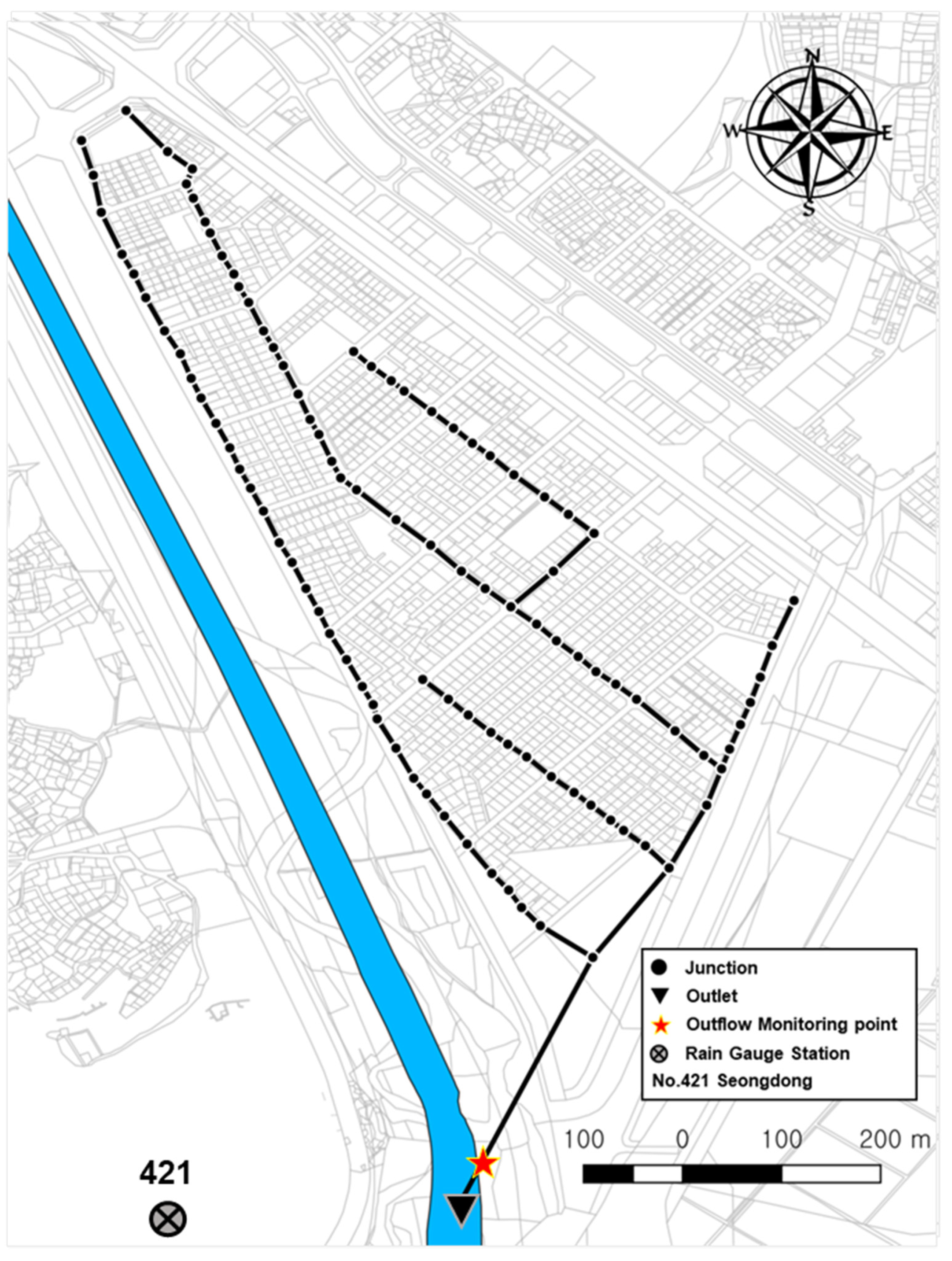
A real drainage area, namely the Yongdap drainage area, was used to demonstrate the proposed MAPC framework. This real drainage area is a representative flooding area located in Seoul, Korea (Figure 1), which receives an average annual rainfall of 1418 mm. This drainage network consists of 101 nodes, 101 links, and 1 outlet. The total pipeline length of the drainage network is 3.546 km, while the total subcatchment area is 0.347 km². The land-use characteristics of this network include 80% residential area and 16 and 4% public and road areas, respectively.

2.2. Datasets

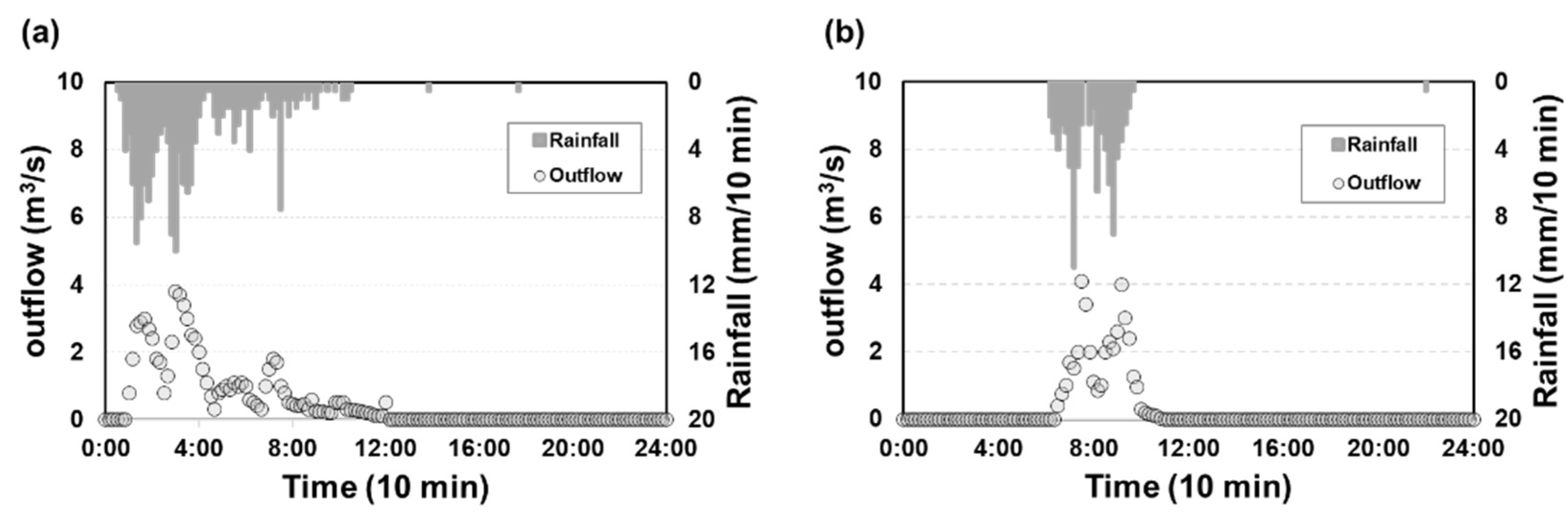
This study utilized rainfall data obtained from 421 gauge-stations located in Seoul, Korea and discharge data obtained at the outflow monitoring point in the Yongdap drainage area. The system discharge data were measured in real-time at the outflow monitoring point. Two types of measurement data were obtained from the Korea Meteorological Administration (https://data.kma.go.kr, accessed on 29 May 2022): rainfall (mm/10 min) and outflow (m³/10 min). One year of historical data for 13–14 July 2013 (i.e., historical urban flood events in Korea) were used to develop the MAPC framework, including rainfall and outflow (e.g., total system discharge). The measurement data (i.e., rainfall (hyetograph) and outflow (hydrograph)) used in this study are shown in Figure 2. Notably, two rainfall events were considered to calibrate and validate the results obtained using the MAPC framework.

3. Modeling Methodology

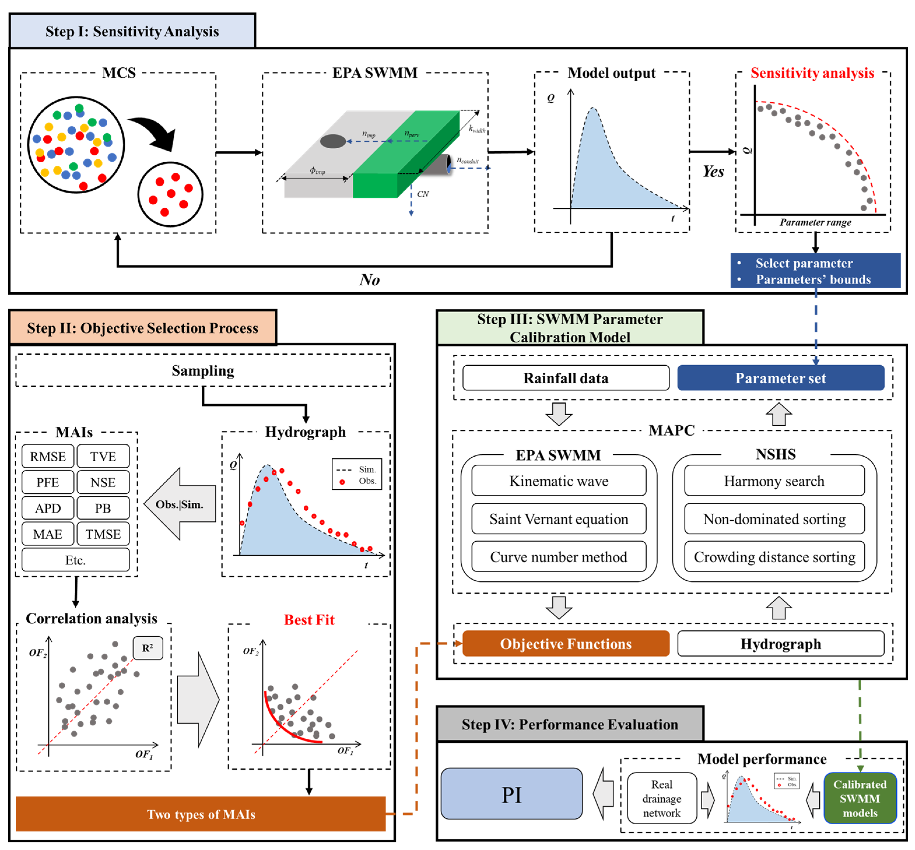
The MAPC framework was developed using NSHS linked with SWMM and consists of four steps (Figure 3). Figure 3 shows a flowchart of the proposed MAPC framework. Subsequent sections describe the details of SWMM, sensitivity analysis (SA), objective selection process (OSP), NSHS, and the proposed SWMM parameter-calibration model and PI.

First, the impact of the relationship between all the parameters and the output in the given UDS model was identified (Step I). Second, the correlation between various model accuracy indicators (MAIs) was confirmed using correlation analysis, and a visual inspection was performed to select two competing objectives to be considered in the proposed SWMM parameter-calibration model (Step II). Third, model calibration was performed based on several parameters and two MAIs (i.e., objective functions) obtained in Steps I and II, respectively (Step III). Finally, based on the calibrated parameters obtained from the SWMM parameter-calibration model for evaluating model accuracy (e.g., model validation), the model results were compared using a predefined performance indicator (PI) (Step IV).

3.1. Stormwater Management Model (SWMM)

The SWMM was first proposed by the United States Environmental Protection Agency and is a rainfall-rainfall hydrological-hydraulic simulation UDS model [10,11]. It has two characteristics: (1) hydrological runoff and (2) hydraulic runoff. The differences in runoff characteristics are driven by climate, land cover, impervious and pervious configurations, pervious area soil types, network topology, and pipe characteristics [28]. Hydrological runoff is a computed path that connects subcatchments between the runoff outlets (e.g., nodes). In contrast, hydraulic runoff is routed downstream via the urban drainage network that connects the node (i.e., hydrological runoff outlet) between an urban river. In SWMM, the rainfall-runoff hydrological-hydraulic simulation is computed using a nonlinear reservoir routing method [29].

The proposed framework was developed on the basis of several SWMM parameters. However, the SWMM parameters used in this study cannot be measured absolutely in the real world. Consequently, the MAPC framework proposed herein considers several sensitive and effective SWMM parameters that require model calibration.

3.2. Step I: Sensitivity Analysis (SA)

SA is a statistical analysis tool that quantifies the impact relationship between input and output in a given model [30,31,32]. It is a process by which different components of a model, such as parameters, forcing inputs, and model structure (e.g., grid resolution in distributed models), are perturbed, and the resulting data are subsequently evaluated to identify the factors that cause the largest variability in the model outputs [33]. For example, SA can be used to determine the model parameters that have the greatest impact on predictions to ensure that calibration efforts are focused on the most critical parameters [34,35]. In recent decades, SA has been widely used to identify the most important parameter depending on the parameters in most UDS calibration studies [36].

SA was performed using Monte Carlo sampling (MCS). To construct the SWMM parameter-calibration model, preselected parameters were identified via the SA approach. Accordingly, uniform random sampling within the predefined upper and lower boundary of parameters, which is determined by physically based model characteristics and engineering knowledge, was used to generate random parameter sets based on the MCS. The generated parameter sets were input into the SWMM, and the outputs (i.e., total system discharge) of each parameter set were obtained. To demonstrate the impact of the relationship between the input and output variables, a scatter plot was generated to present the potential correlations (e.g., linear and nonlinear). Finally, the range of output (i.e., total system discharge) according to all parameters was quantified and presented as a box-whisker plot.

The impact relationship between the outflow and each parameter was then investigated using SA. Six parameters were employed to perform SA, and their information (i.e., parameters, descriptions, and prior distributions) is summarized in

Table 1. Summary of the parameters used for the proposed MAPC model.

Parameter	Description (Unit)	Prior Distribution
kwidth	Hillslope width factor (m)	*U (30, 170)
Фimp	Impervious fraction in urban land (%)	*U (60, 100)
CN	Curve number (-)	*U (53, 75)
nimp	Manning’s n on impervious (-)	*U (0.03, 0.05)
nperv	Manning’s n on pervious (-)	*U (0.03, 0.05)
nconduit	Manning’s n on pipe roughness (-)	*U (0.011, 0.017)

Note: *U (a, b) means the uniform distribution, a < b where is beginning of the interval and b is the end of the interval.

. Notably, all parameters in this study were strictly investigated using literature related to SWMM-SA and/or calibration studies [23,36,37,38,39]. Furthermore, if the SWMM parameters in SA have no effect, their parameters are not considered for the SWMM parameter-calibration model (Step III).

3.3. Step II: Objective Selection Process (OSP)

The accuracy of the proposed SWMM parameter-calibration model was evaluated by comparing the observed and simulated outflow (i.e., total system discharge) values at the outlet (the urban drainage network outlet is depicted as a black inverted triangle in Figure 1). The SWMM parameters were calibrated to minimize model uncertainty, which could be considered a physically based model (i.e., SWMM). Various MAIs have been formulated and used in the SWMM automatic parameter-calibration problem of the UDS model.

Table 2. Model accuracy indicators used in the proposed MAPC framework.

Indicator Names (Abbreviations)	Formulations
Root-mean-square error (RMSE)	$\sqrt{\frac{1}{n}{\displaystyle \sum _{t=1}^1}{\left(Q_{obs\left(t\right)}-Q_{sim\left(t\right)}\right)}^2}$
Total volume error (TVE)	$\frac{1}{Q_{sim\left(t\right)}}{\displaystyle \sum _{t=1}^1}\left|Q_{obs\left(t\right)}-Q_{sim\left(t\right)}\right|$
RMSE of peak flow error (PFE)	$\sqrt{\frac{1}{n_P}{\displaystyle \sum _{t=1}^1}{\left(P_{obs}-P_{sim}\right)}^2}$
Nash-Sutcliffe efficiency coefficient (NSE)	$1-\frac{\frac{1}{n}{\sum }_{t=1}^1{\left(Q_{obs\left(t\right)}-Q_{sim\left(t\right)}\right)}^2}{\frac{1}{n}{\sum }_{t=1}^1{\left(Q_{obs\left(t\right)}-\overline{Q_{obs}}\right)}^2}$
Absolute peak difference (APD)	$\left|\underset{1\le t\le n }{\max }(O_{obs\left(t\right)})-\underset{1\le t\le n }{\max }(O_{sim\left(t\right)})\right|$
Percent bias (PB)	$100\times \left|\frac{\frac{1}{n}({\sum }_{t=1}^n{Q}_{obs\left(t\right)}-{\sum }_{t=1}^n{Q}_{sim\left(t\right)})}{\frac{1}{n}{\sum }_{t=1}^n{Q}_{obs\left(t\right)}}\right|$
Mean absolute error (MAE)	$\frac{1}{n}{\displaystyle \sum _{t=1}^n}\left|Q_{obs\left(t\right)}-Q_{sim\left(t\right)}\right|$
Maximum absolute error (MaxAE)	$\underset{1\le t\le n }{\max }\left|O_{obs\left(t\right)}-Q_{sim\left(t\right)}\right|$
Total mean squared error (TMSE)	$\frac{1}{n}{\displaystyle \sum _{t=1}^1}\left(Q_{obs}\left(t\right)-Q_{sim}\left(t\right)\right)$

Note: $Q_{Obs\left(t\right)}$ is the observed outflow at time $t$; $Q_{sim\left(t\right)}$ is the simulated outflow at time $t$; $\overline{Q_{obs}}$ is the mean value of the observed outflow during the period from t = 1 to n; $P_{obs}$ is the observed peak outflow; and $P_{sim}$ is the simulated peak outflow.

summarizes several MAIs used by the National Weather Service for calibration of the Sacramento soil moisture accounting (SAC-SMA) model [40]. Several indicators (i.e., Nash-Sutcliffe efficiency coefficient, root-mean-square error, total mean squared error, and total volume error) have also been widely used in hydrological model calibration studies [23,41,42,43]. To develop the SWMM parameter-calibration model, the relationship between one indicator with the other indicators among the MAIs (i.e., objective functions) considered in this study was identified. Note that the MAIs formulae presented in Table 2 are well known by most hydrology researchers and do not require separate citations.

To construct a SWMM parameter-calibration model, two competing MAIs must be identified. The two correlated indicators should not be simultaneously considered in the model because minimizing/maximizing one indicator would have the same effect on the other indicator [40]. Accordingly, uniform random sampling within the upper and lower bounds of the parameters, which is conducted based on physical reasonability, engineering knowledge, and Monte Carlo simulations (MCS), was used to generate random parameter sets. A simulated hydrograph was obtained from the rainfall-runoff simulation using each generated parameter set, with the calculated MAIs listed in Table 1. Finally, a scatter plot of each pair of MAIs in Table 1 and their linear regression lines were drawn and inspected to detect potential correlations. Note that the linear regression line and R-squared coefficient (R²) were used to confirm inherent correlation between MAIs. A set of two MAIs should not be simultaneously considered in the multiobjective calibration model if they are highly correlated and aligned with the regression line (i.e., high R-squared coefficient). Considering one indicator in the objective function can automatically minimize/maximize the other indicator by their inherent correlation without explicitly and additionally considering the other in the formulation.

3.4. Step III: SWMM Parameter-Calibration Model

The SWMM parameter-calibration model proposed in this study explores for an optimal parameter set based on NSHS. The NSHS is a multiobjective optimization method, considering the nondominated sorting and crowding distance approach [44,45,46] within the harmony search algorithm developed by Geem et al. [47]. The harmony search algorithm is a metaheuristic algorithm based on the musical performance process that occurs when a musician searches for a better state of harmony during jazz improvisation. The NSHS, which includes the nondominated sorting and crowding distance approach, was used with the harmony search algorithm in this study. In addition, various water engineering studies have shown that this algorithm is better than conventional optimization algorithms with respect to the convergence performance [48].

The SWMM parameter-calibration model searches for the trade-off relationship between the MAI pair selected via the goal selection procedure. The values of these MAIs were determined using the SWMM parameters identified in SA. Jung et al. [40] formulated the multiobjective parameter-calibration model as follows:

$$\{\begin{array}{c}\mathrm{Minimize} f_1=\mathrm{MAI}1\left(x_n\right)\\ \mathrm{Minimize} f_2=\mathrm{MAI}2\left(x_n\right)\end{array}$$

(1)

where $\mathrm{MAI}1$ and $\mathrm{MAI}2$ are a pair of MAIs optimized by the multiobjective parameter-calibration model, $x$ is the model parameter that determines the MAI value, and $n$ is the number of parameter types.

The SWMM parameter-calibration model provides parameter sets in which the MAI pair has a trade-off relationship as a Pareto-optimal solution. The SWMM constructed in this study simulates the outflow based on the parameters suggested by the SWMM parameter-calibration model. The result is then compared with the observed outflow curve to examine the performance of the MAPC framework proposed in this study.

3.5. Step IV: Performance Evaluation

The Pareto-optimal solution obtained in Step III was evaluated using a predefined PI. The PI was only selected as a representative indicator in the aforementioned MAIs (summarized in Table 2). In addition, note that several indicators can be excluded for defining MAI 1 and 2, respectively (e.g., objective functions 1 and 2 in Step III). The final optimal solutions obtained from the proposed model were compared and evaluated with other optimal solutions using the PI.

4. Application Results

4.1. Sensitivity Analysis (SA)

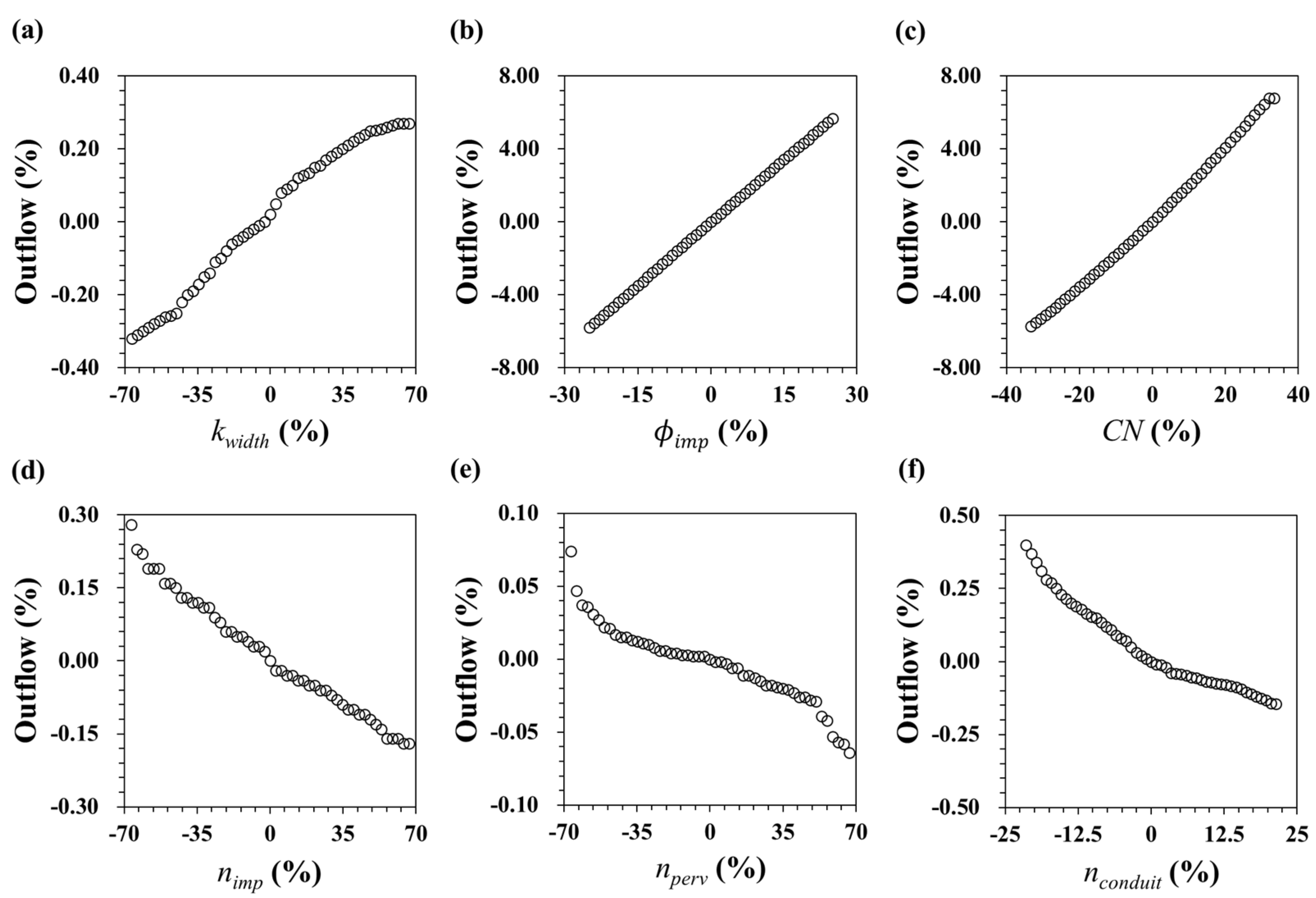
In this section, the change in total outflow (i.e., sensitivity) based on the parameters is examined, and the types of parameters to be entered in the SWMM parameter-calibration model are determined. SA was performed according to the MCS, and the individual parameters had different values. In this study, 100 of the 500 SWMM simulation results were extracted. Figure 4 shows the scatterplots of the SWMM outputs based on the parameters extracted from the MCS.

k_width, Ф_imp, and CN were identified as the parameters that increase the outflow. k_width is multiplied when calculating the surface runoff in the SWMM governing equation [29]. Therefore, an increase in k_width may lead to an increase in outflow. An increase in Ф_imp and CN, which determine the infiltration amount, influences the increase in outflow [49]. As n_imp, n_perv, and n_conduit increase, the total outflow decreases. As n_imp, n_perv, and n_conduit increase, losses caused by friction occur [50], which reduce the outflow. Figure 4 shows that all the parameters considered in the sensitivity analysis were consistently altered. Therefore, even if the parameter search range is entered as a continuous range in the SWMM parameter-calibration model, this range would not have a large impact on the result [39].

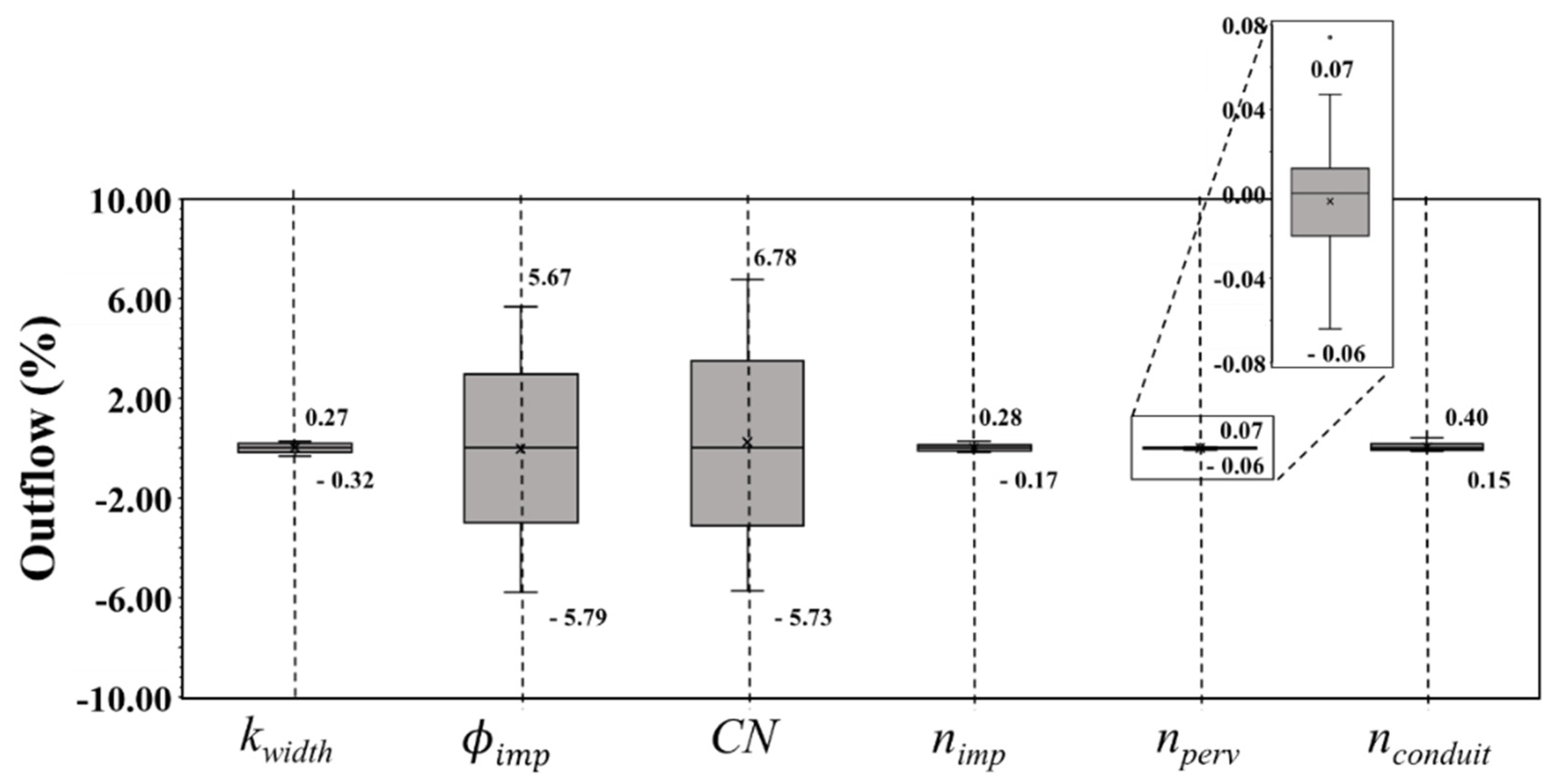
Figure 5 shows a box and whisker plot of the outflow variation for each parameter. Ф_imp and CN were found to be highly sensitive to the model output. These two parameters directly affect the amount of rainfall that is converted to surface runoff through infiltration. In contrast, k_width, n_imp, n_perv, and n_conduit did not show large changes in outflow compared to parameter changes. However, because these parameters affect the peak outflow, further investigation is required. When the characteristics of the study network (urban catchment) were considered, a lack of influence of k_width, n_imp, and n_conduit could not be determined. Although outliers were found for n_perv, their impact was not large because the target network had the characteristic of a high infiltration rate. Therefore, n_perv was excluded from the parameters calibrated using the SWMM parameter-calibration model.

4.2. Selection of Two Objectives

The SWMM parameter-calibration model searches for the optimal solution set for the two goals that form a trade-off relationship. Therefore, this section describes the determination of the two MAIs to be used as objective functions in the SWMM parameter-calibration model. The two objective functions were selected as follows: (1) First, various MAIs used to check the hydrological modeling performance were selected, and their applicability to SWMM was examined. (2) Based on the SA results, the parameters were randomly confounded to create multiple SWMM runs. (3) Samples were extracted through sampling, and the MAIs of each sample SWMM were calculated. (4) The MAIs were displayed and examined using scatterplots, regression lines, and coefficients of determination (R²).

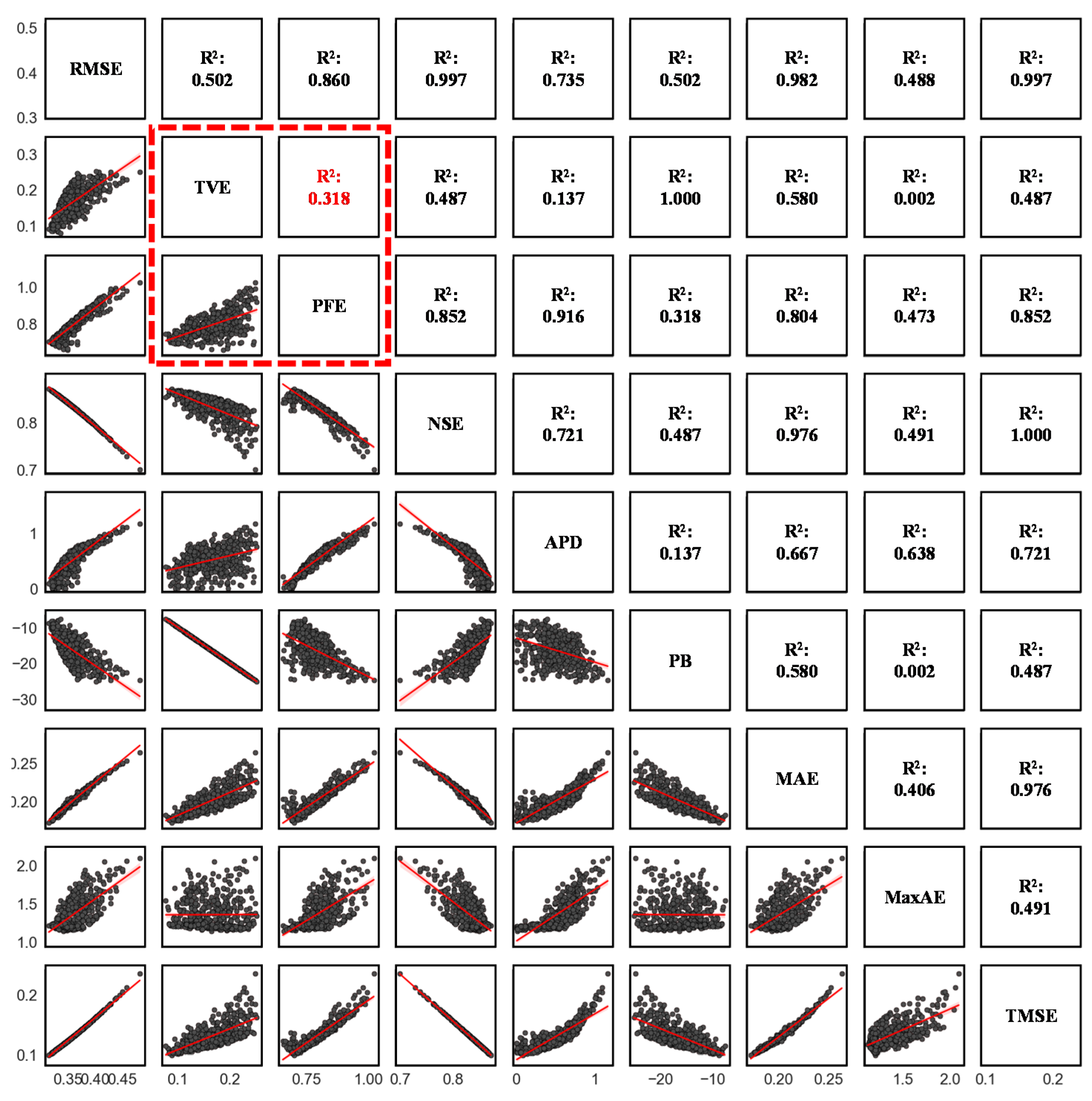
Figure 6 shows scatterplots, linear regression lines, and R² for the relationships between 500 MAI calculation results extracted randomly from 1000 SWMM runs with randomly adjusted parameters. In the results, for a pair of MAIs considered good, objective functions of the SWMM parameter-calibration model should be depicted in a space where the trade-off relationship shows the optimum value of each MAI. Among the pairs of MAIs considered in this study, 18 sets exist, including RMSE-PB, RMSE-MaxAE, TVE-PFE, and TVE-NSE, which can be selected as two objective functions. Most pairs of MAIs show the trade-off relationship on the lower left side. However, if NSE is included, the trade-off relationship is shown on the upper right side; this is because among the MAIs considered in this study, NSE is the only MAI with good model performance when large. The coefficient of determination (R²) of these sets is between 0.1 and 0.8.

In this study, TVE and PFE were selected as the two objective functions of the SWMM parameter-calibration model. The two MAIs have the same unit (m³/s), enabling an easy analysis of the derived solutions. Furthermore, as the MAIs show the characteristics of the outflow curve intuitively, the hydrographs of the validation and calibration SWMMs are expected to be easily examined.

4.3. Comparison between Pareto-Optimal Solutions

Pareto-optimal solutions of the SWMM parameter-calibration model were assessed to examine the calibrated SWMM. First, the targets to be examined were selected from among the Pareto-optimal solutions provided by the SWMM parameter-calibration model. The hydrograph simulation result of the SWMM, in which the selected parameter combination was entered, was finally compared to the observed outflow.

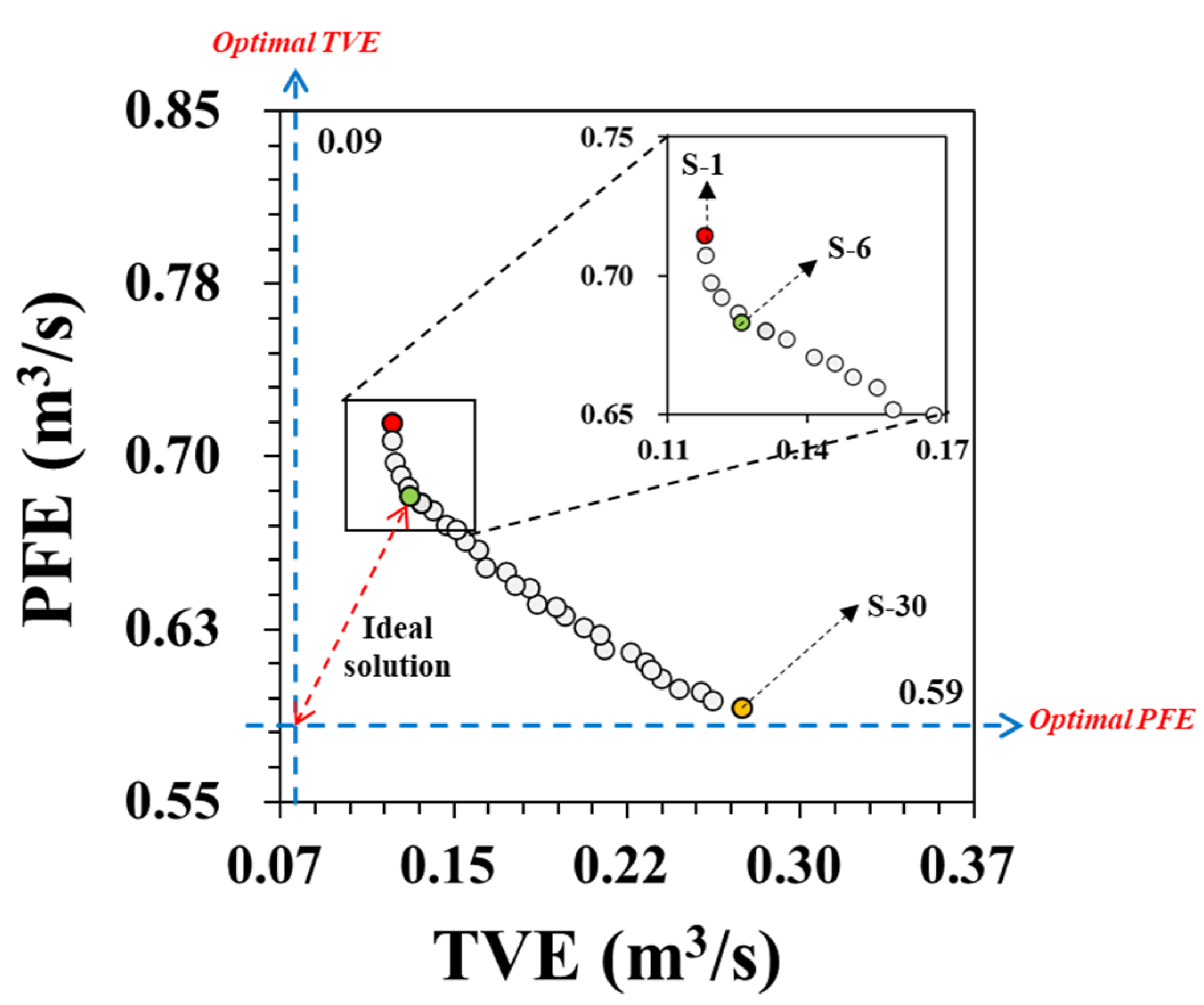
Figure 7 shows the Pareto-optimal solutions provided by the SWMM parameter-calibration model. A total of 30 solutions were obtained; however, examining all solutions is inefficient. Therefore, we used the reference solution to determine the solution that should be examined (the reference solution refers to the solution derived by optimizing only one of the two objective functions (TVE and PFE)). The reference solution of each objective function is represented by a blue line in Figure 7 (TVE = 0.09 m³/s, PFE = 0.59 m³/s). In this study, three solutions (S-1, S-6, and S-30) were selected based on the reference solutions. S-1 and S-30 are the closest solutions to the reference solutions of TVE and PFE, respectively. S-6 is the ideal solution to the intersection point where the reference solutions meet the Pareto-optimal solutions.

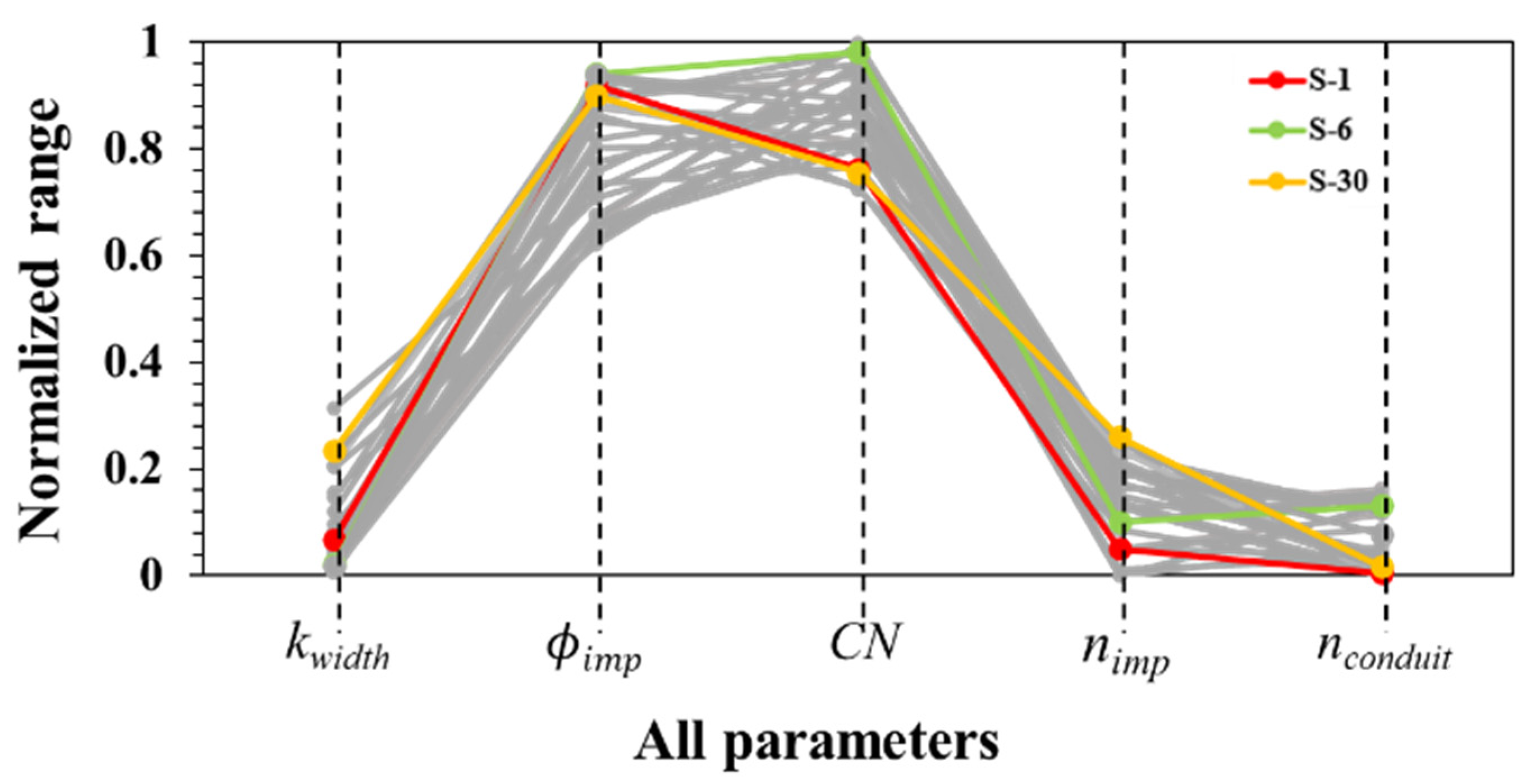
Figure 8 shows the calibration results of the Pareto-optimal solutions, which were normalized based on the maximum and minimum values of the parameter search range. In S-30, k_width and n_imp are highly calibrated compared with the other solutions. Thus, it was confirmed that the peak flow of the study network can be adjusted using k_width and n_imp. As the characteristics of the urban network were well reflected, Ф_imp of all solutions, including S-1, S-6, and S-30, was calibrated to be high. CN and n_conduit were calibrated to be high in S-6, unlike S-1 and S-30, implying that CN and n_conduit are parameters that play a decisive role in the search for the trade-off section between TVE and PFE. The overall results revealed that the calibrated value of each parameter obtained from the Pareto-optimal solutions displayed a consistent tendency for the system characteristics (e.g., hillslope width factor, curve number, etc.).

4.4. Multiobjective Calibration and Validation

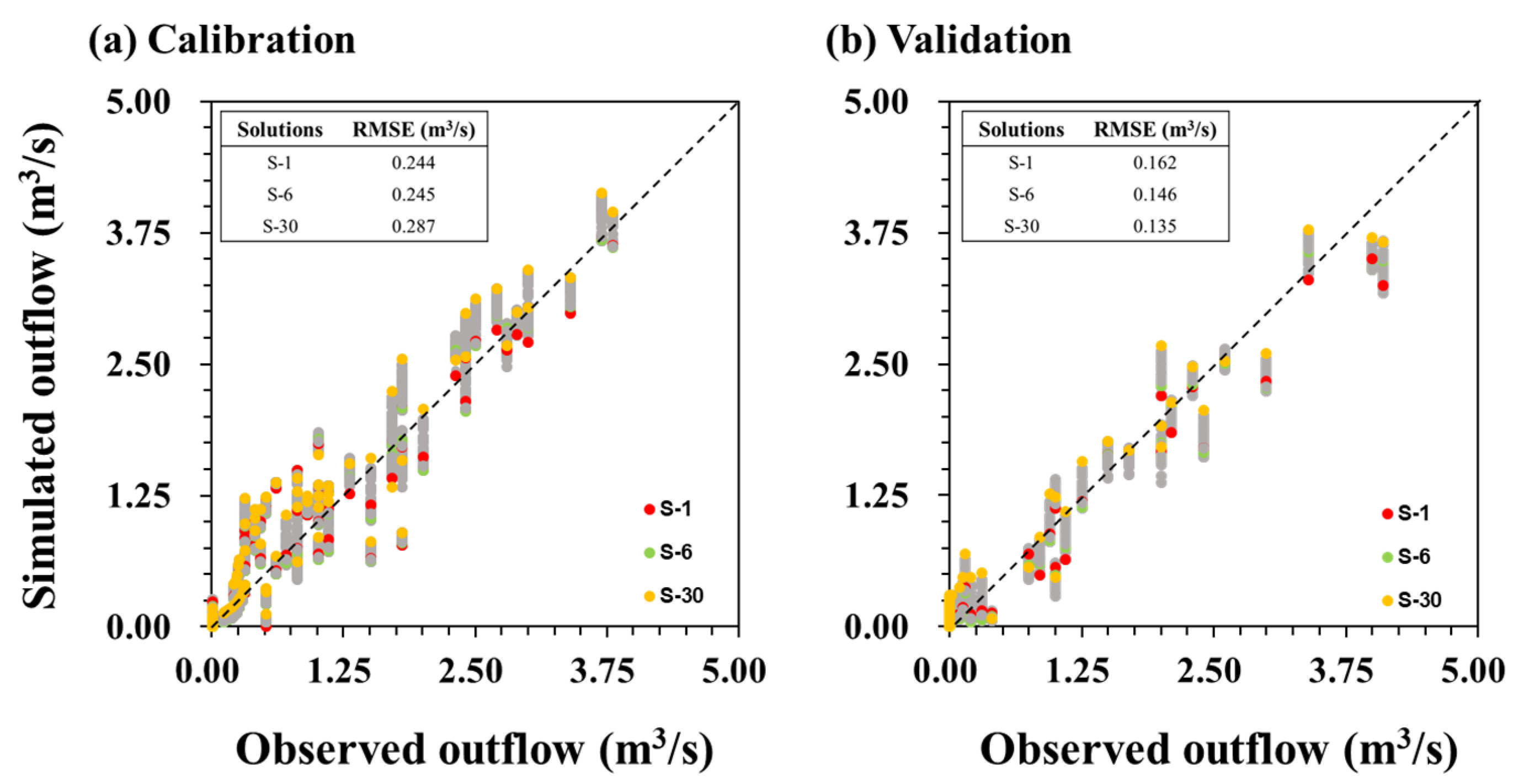
Figure 9 compares the simulated outflow from the calibrated SWMM with the observed outflow. S-1 shows the lowest RMSE of 0.244 for the observed outflow used for calibration (Figure 9a). However, the RMSE for the validation (Figure 9b) observed outflow is 0.162, which is the worst performance among all. In contrast, S-30 shows the highest RMSE for the calibration observed outflow of 0.287, but the result for the validation observed outflow is the best at 0.135. The ideal solution, S-6, has RMSEs of 0.245 and 0.146 for the two observed outflows. The RMSE of S-6 is not significantly different from that of the solution that performed well for each observed outflow. The hydrograph used for calibration has a longer outflow than that used for validation.

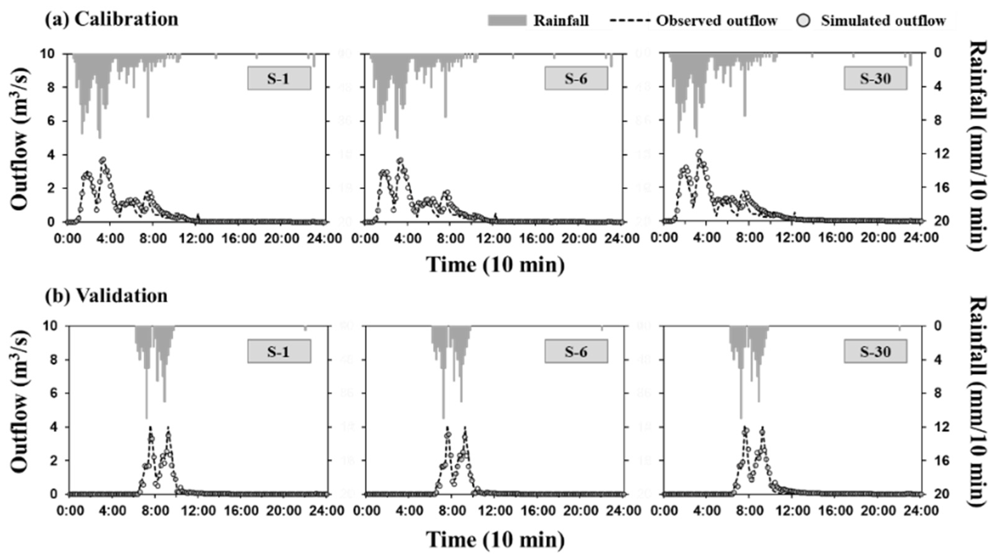
This is why the RMSE values in Figure 10a and Figure 10b show a large overall difference result, respectively. Figure 10 shows graphs comparing the simulated and observed outflows for the validation and calibration rainfalls of S-1, S-6, and S-30. Visually, all three solutions simulated outflows that are similar to the observed outflow. Four peaks were observed, and the peak values were found to be not equal in the rainfall events used for calibration. In S-1 and S-6, where TVE is low, the hydrograph model is adequately simulated. For S-30, the simulated outflow is large, and the outflow variation in the section of the third peak (5:00–7:00) is barely simulated. However, in a network where the hydrograph is simple and the peaks occur evenly, as in the validation hydrograph, the simulated outflow is closer to the observed outflow. When a peak occurs, the simulation results for not only the outflow but also the time of occurrence are close to the observed values. However, for S-1, the peak occurrence time is not accurate, and an under-simulated hydrograph is shown.

This implies that a solution with low TVE should be selected for a complex rainfall event. Conversely, for a simple rainfall event, a solution with a low PFE is a more advantageous choice. In a real drainage network, how rainfall falls is unknown [51]. Therefore, a SWMM that can respond flexibly to various rainfall events is required. S-6 shows a hydrograph that adequately reflects the characteristics of S-1 and S-30. The ideal solution, such as S-6, is thus a SWMM that can respond to various rainfall events.

5. Summary and Conclusions

This study proposed a multiobjective automatic parameter-calibration (MAPC) framework based on the stormwater management model (SWMM). The proposed MAPC framework consists of four steps: sensitivity analysis (Step I), objective selection (Step II), SWMM parameter calibration (Step III), and comparison with Pareto-optimal solutions using performance indicator (Step IV). The proposed MAPC framework was verified using the Yongdap drainage network in Seoul, South Korea.

In summary, the calibrated parameter sets obtained from the Pareto-optimal solutions displayed a consistent tendency based on model performance. The simulated outflow obtained by the proposed framework was confirmed to be almost similar to the observed outflow. In fact, the root-mean-square error, computed using all optimal solutions, was in the range of 0.244–0.287 (calibration model) and 0.135–0.162 (validation model). The resultant MAPC framework demonstrated that the system characteristics (such as percent of impervious area and hillslope) and problems in UDS design, planning, and management can be well reflected by the corresponding model. The MAPC framework provided a series of processes for UDS modeling and is expected to contribute to UDS modeling sustainability.

This study has several limitations that may be addressed in future research. First, in a real drainage area, each parameter has a different value depending on the model components (e.g., links, nodes, and subcatchments). However, this study considered that the components have uniform distribution for each parameter. Second, this study considered only two objective functions (i.e., peak flow and total volume errors), such that only specific characteristics of the optimal solution are localized in two objective functions. In addition, further study must investigate three or more objective functions (e.g., model accuracy indicators) to improve the SWMM parameter-calibration model compared to the proposed framework. Third, this study focused on matching the outflow hydrographs at the network outlet with real-time measurements. A follow-up study can calibrate the overland flow from each sub-catchment by considering the corresponding measurements at each manhole (i.e., sub-catchment outlet). Finally, although the proposed MAPC framework focused only on hydrological parameters, it can be enhanced to obtain an advanced MAPC framework by considering hydrological, hydraulic, and water quality parameters simultaneously.

References

- Afshar, M.H.; Marino, M.A. Application of an ant algorithm for layout optimization of tree networks. Eng. Optim. 2006, 38, 353–369. [Google Scholar] [CrossRef]
- Dong, X.; Guo, H.; Zeng, S. Enhancing future resilience in urban drainage system: Green versus grey infrastructure. Water Res. 2017, 124, 280–289. [Google Scholar] [CrossRef] [PubMed]
- Semadeni-Davies, A.; Hernebring, C.; Svensson, G.; Gustafsson, L.G. The impacts of climate change and urbanisation on drainage in Helsingborg, Sweden: Combined sewer system. J. Hydrol. 2008, 350, 100–113. [Google Scholar] [CrossRef]
- Zhou, Q. A review of sustainable urban drainage systems considering the climate change and urbanization impacts. Water 2014, 6, 976–992. [Google Scholar] [CrossRef]
- Yazdanfar, Z.; Sharma, A. Urban drainage system planning and design–challenges with climate change and urbanization: A review. Water. Sci. Technol. 2015, 72, 165–179. [Google Scholar] [CrossRef] [Green Version]
- Vojinovic, Z.; Sahlu, S.; Torres, A.S.; Seyoum, S.D.; Anvarifar, F.; Matungulu, H.; Barreto, W.; Savic, D.; Kapelan, Z. Multi-objective rehabilitation of urban drainage systems under uncertainties. J. Hydroinform. 2014, 16, 1044–1061. [Google Scholar] [CrossRef]
- Notaro, V.; Liuzzo, L.; Freni, G.; la Loggia, G. Uncertainty analysis in the evaluation of extreme rainfall trends and its implications on urban drainage system design. Water 2015, 7, 6931–6945. [Google Scholar] [CrossRef]
- Li, C.; Wang, W.; Xiong, J.; Chen, P. Sensitivity analysis for urban drainage modeling using mutual information. Entropy 2014, 16, 5738–5752. [Google Scholar] [CrossRef]
- Gironás, J.; Roesner, L.A.; Rossman, L.A.; Davis, J. A new applications manual for the Storm Water Management Model (SWMM). Environ. Model. Soft. 2010, 25, 813–814. [Google Scholar] [CrossRef]
- Hossain, S.; Hewa, G.A.; Wella-Hewage, S. A comparison of continuous and event-based rainfall–runoff (RR) modelling using EPA-SWMM. Water 2019, 11, 611. [Google Scholar] [CrossRef] [Green Version]
- Sun, C.; Lorenz Svensen, J.; Borup, M.; Puig, V.; Cembrano, G.; Vezzaro, L. An MPC-enabled SWMM implementation of the Astlingen RTC benchmarking network. Water 2020, 12, 1034. [Google Scholar] [CrossRef] [Green Version]
- Annus, I.; Vassiljev, A.; Kändler, N.; Kaur, K. Automatic calibration module for an urban drainage system model. Water 2021, 13, 1419. [Google Scholar] [CrossRef]
- Cooper, V.A.; Nguyen, V.T.V.; Nicell, J.A. Calibration of conceptual rainfall–runoff models using global optimisation methods with hydrologic process-based parameter constraints. J. Hydrol. 2007, 334, 455–466. [Google Scholar] [CrossRef]
- Niemi, T.J.; Kokkonen, T.; Sillanpää, N.; Setälä, H.; Koivusalo, H. Automated urban rainfall–runoff model generation with detailed land cover and flow routing. J. Hydrol. Eng. 2019, 24, 04019011. [Google Scholar] [CrossRef] [Green Version]
- Yapo, P.O.; Gupta, H.V.; Sorooshian, S. Automatic calibration of conceptual rainfall-runoff models: Sensitivity to calibration data. J. Hydrol. 1996, 181, 23–48. [Google Scholar] [CrossRef]
- Jin, X.; Jiang, Y.; Wu, W.; Jin, J. Automatic calibration of SWMM model with adaptive genetic algorithm. In Proceedings of the International Symposium on Water Resource and Environmental Protection, Xi’an, China, 20–22 May 2011. [Google Scholar]
- Wan, B.; James, W. SWMM calibration using genetic algorithms. In Proceedings of the Ninth International Conference on Urban Drainage, Portland, OR, USA, 8–13 September 2002; American Society of Civil Engineers: Reston, VA, USA, 2002; pp. 1–14. [Google Scholar]
- Tobio, J.A.S.; Maniquiz-Redillas, M.C.; Kim, L.H. Optimization of the design of an urban runoff treatment system using stormwater management model (SWMM). Desalin. Water. Treat. 2015, 53, 3134–3141. [Google Scholar] [CrossRef]
- Dent, S.; Hanna, R.B.; Wright, L.T. Automated calibration using optimization techniques with SWMM RUNOFF. J. Water. Manag. Model. 2014, 23, 45–52. [Google Scholar] [CrossRef] [Green Version]
- Kollat, J.B.; Reed, P.M.; Wagener, T. When are multiobjective calibration trade-offs in hydrologic models meaningful? Water. Resour. Res. 2012, 48, W03520. [Google Scholar] [CrossRef]
- Reed, P.M.; Hadka, D.; Herman, J.D.; Kasprzyk, J.R.; Kollat, J.B. Evolutionary multiobjective optimization in water resources: The past, present, and future. Adv. Water. Resour. 2013, 51, 438–456. [Google Scholar] [CrossRef] [Green Version]
- Efstratiadis, A.; Koutsoyiannis, D. One decade of multi-objective calibration approaches in hydrological modelling: A review. Hydrolog. Sci. J. 2010, 55, 58–78. [Google Scholar] [CrossRef] [Green Version]
- Gutierrez, J.C.T.; Adamatti, D.S.; Bravo, J.M. A new stopping criterion for multi-objective evolutionary algorithms: Application in the calibration of a hydrologic model. Comput. Geosci. 2019, 23, 1219–1235. [Google Scholar] [CrossRef]
- Saavedra, D.; Mendoza, P.; Addor, N.; Llauca, H.; Vargas, X. A multi-objective approach to select hydrological models and constrain structural uncertainties for climate impact assessments. Hydrolog. Process. 2022, 36, e14446. [Google Scholar] [CrossRef]
- Perin, R.; Trigatti, M.; Nicolini, M.; Campolo, M.; Goi, D. Automated calibration of the EPA-SWMM model for a small suburban catchment using PEST: A case study. Environ. Monit. Assess. 2020, 192, 374. [Google Scholar] [CrossRef] [PubMed]
- Swathi, V.; Srinivasa Raju, K.; Varma, M.R.R.; Sai Veena, S. Automatic calibration of SWMM using NSGA-III and the effects of delineation scale on an urban catchment. J. Hydroinform. 2019, 21, 781–797. [Google Scholar] [CrossRef]
- Behrouz, M.S.; Zhu, Z.; Matott, L.S.; Rabideau, A.J. A new tool for automatic calibration of the Storm Water Management Model (SWMM). J. Hydrol. 2020, 581, 124436. [Google Scholar] [CrossRef]
- Sytsma, A.; Crompton, O.; Panos, C.; Thompson, S.; Mathias Kondolf, G. Quantifying the uncertainty created by non-transferable model calibrations across climate and land cover scenarios: A case study with SWMM. Water Res. Res. 2022, 58. [Google Scholar] [CrossRef]
- Rossman, L.A.; Huber, W.C. Storm Water Management Model Reference Manual Volume I–Hydrology; Revised; US Environmental Protection Agency: Cincinnati, OH, USA, 2016.
- Madsen, H. Parameter estimation in distributed hydrological catchment modelling using automatic calibration with multiple objectives. Adv. Water Resour. 2003, 26, 205–216. [Google Scholar] [CrossRef]
- Akdoğan, Z.; Güven, B. Assessing the sensitivity of SWMM to variations in hydrological and hydraulic parameters: A case study for the city of Istanbul. Glob. NEST J. 2016, 18, 831–841. [Google Scholar]
- Tsai, L.Y.; Chen, C.F.; Fan, C.H.; Lin, J.Y. Using the HSPF and SWMM models in a high pervious watershed and estimating their parameter sensitivity. Water 2017, 9, 780. [Google Scholar] [CrossRef] [Green Version]
- Ahmadisharaf, E.; Camacho, R.A.; Zhang, H.X.; Hantush, M.M.; Mohamoud, Y.M. Calibration and validation of watershed models and advances in uncertainty analysis in TMDL studies. J. Hydrol. Eng. 2019, 24, 03119001. [Google Scholar] [CrossRef]
- Campolongo, F.; Saltelli, A.; Tarantola, S. Sensitivity analysis as an ingredient of modeling. Stat. Sci. 2000, 15, 377–395. [Google Scholar] [CrossRef]
- White, K.L.; Chaubey, I. Sensitivity analysis, calibration, and validations for a multisite and multivariable SWAT model. J. Am. Water Res. Assoc. 2005, 41, 1077–1089. [Google Scholar] [CrossRef]
- James, W. Rules for Responsible Modeling; CHI: Guelph, ON, Canada, 2005. [Google Scholar]
- Barco, J.; Wong, K.M.; Stenstrom, M.K. Automatic calibration of the US EPA SWMM model for a large urban catchment. J. Hydraul. Eng. 2008, 134, 466–474. [Google Scholar] [CrossRef]
- Lim, O.; Yoo, D.G.; Lee, E.H.; Kim, J.H. A study on the parameter estimation of sewer network model using sewer level data. J. Korean Soc. Hazard. Mitig. 2018, 18, 261–269. [Google Scholar] [CrossRef] [Green Version]
- Chung, G.; Yeon, J.S.; Sim, K.B.; Kim, E.S. The sensitivity and uncertainty analysis of SWMM water quality parameters. J. Korean Soc. Hazard. Mitig. 2015, 15, 247–253. [Google Scholar] [CrossRef] [Green Version]
- Jung, D.; Choi, Y.; Kim, J. Multiobjective automatic parameter calibration of a hydrological model. Water 2017, 9, 187. [Google Scholar] [CrossRef] [Green Version]
- Krebs, G.; Kokkonen, T.; Valtanen, M.; Koivusalo, H.; Setälä, H. A high resolution application of a stormwater management model (SWMM) using genetic parameter optimization. Urban Water J. 2013, 10, 394–410. [Google Scholar] [CrossRef]
- Liong, S.Y.; Chan, W.T.; Lum, L.H. Knowledge-based system for SWMM runoff component calibration. J. Water Resour. Plan. Manag. 1991, 117, 507–524. [Google Scholar] [CrossRef]
- Khu, S.T.; Madsen, H. Multiobjective calibration with Pareto preference ordering: An application to rainfall-runoff model calibration. Water Resour. Res. 2005, 41. [Google Scholar] [CrossRef]
- Yazdi, J.; Sadollah, A.; Lee, E.H.; Yoo, D.G.; Kim, J.H. Application of multi-objective evolutionary algorithms for the rehabilitation of storm sewer pipe networks. J. Flood Risk Manag. 2017, 10, 326–338. [Google Scholar] [CrossRef]
- Kougias, I.P.; Theodossiou, N.P. Multiobjective pump scheduling optimization using harmony search algorithm (HSA) and polyphonic HSA. Water Resour. Manag. 2013, 27, 1249–1261. [Google Scholar] [CrossRef]
- Deb, K.; Pratap, A.; Agarwal, S.; Meyarivan, T. A fast and elitist multiobjective genetic algorithm: NSGA-II. IEEE Trans. Evol. Comput. 2002, 6, 182–197. [Google Scholar] [CrossRef] [Green Version]
- Geem, Z.W.; Kim, J.H.; Loganathan, G.V. A new heuristic optimization algorithm: Harmony search. Simulation 2001, 76, 60–68. [Google Scholar] [CrossRef]
- Yazdi, J.; Choi, Y.H.; Kim, J.H. Non-dominated sorting harmony search differential evolution (NS-HS-DE): A hybrid algorithm for multi-objective design of water distribution networks. Water 2017, 9, 587. [Google Scholar] [CrossRef] [Green Version]
- Bisht, D.S.; Chatterjee, C.; Kalakoti, S.; Upadhyay, P.; Sahoo, M.; Panda, A. Modeling urban floods and drainage using SWMM and MIKE URBAN: A case study. Nat. Hazard. 2016, 84, 749–776. [Google Scholar] [CrossRef]
- Zaghloul, N.A. Flow simulation in circular pipes with variable roughness using SWMM-EXTRAN model. J. Hydraul. Eng. 1998, 124, 73–76. [Google Scholar] [CrossRef]
- Pretorius, H.; James, W.; Smit, J. A strategy for managing deficiencies of SWMM modeling for large undeveloped semi-arid watersheds. J. Water Manag. Model. 2013, R246-01. [Google Scholar] [CrossRef] [Green Version]