
A Quantitative Study on the Identification of Ecosystem Services: Providing and Connecting Areas and Their Impact on Ecosystem Service Assessment

Abstract
:1. Introduction
2. Theoretical Basis
2.1. Definition of Service-Providing, -Connecting, and -Demand Areas
- (1)
- Service-providing areas
- (2)
- Service-connecting areas
- (3)
- Service-demand areas
2.2. Identification Principles of Service-Providing, -Connecting, and -Demand Areas
- (1)
- General principle of service-providing area identification
- (2)
- General principle of service-connecting area identification
- (3)
- General principles of service-demand area identification
3. Methods
3.1. Identification Methods of Service-Providing, -Connecting, and -Demand Areas
3.2. A Quantitative Method on the Impact of Service-Providing, and -Connecting Areas on Ecosystem Service Assessments
- (1)
- The service diversity index comprehensively reflects the diversity of service types provided by service-providing areas and the diversity of service types associated with service-connecting areas within the region, and are recorded as ID (SPA) and ID (SCA), respectively.
- (2)
- The service diversity participation rate comprehensively reflects the contribution rate of the number of types of services undertaken by each regional unit of the service-providing area or service-connecting area to the number of types of ecosystem services provided by the overall regional ecological space, which are recorded as IP (SPA) and IP (SCA), respectively.
- (3)
- The benefit area rate of the service-demand area represents the proportion of the actual benefit area benefited by the service-demand area from the service-providing area (SPA) and the service-connecting area (SCA), which are recorded as %Ben.pro(i) and %Ben.con(i), respectively.
- (4)
- The service benefit contribution rate represents the contribution of the service-providing area and the service-connecting area to the total benefit area of the service-demand area, and are recorded as %IPSP(SPA) and %IPSP(SCA), respectively. The calculation formulas are shown in Formulas (6)–(9):
4. Case Study
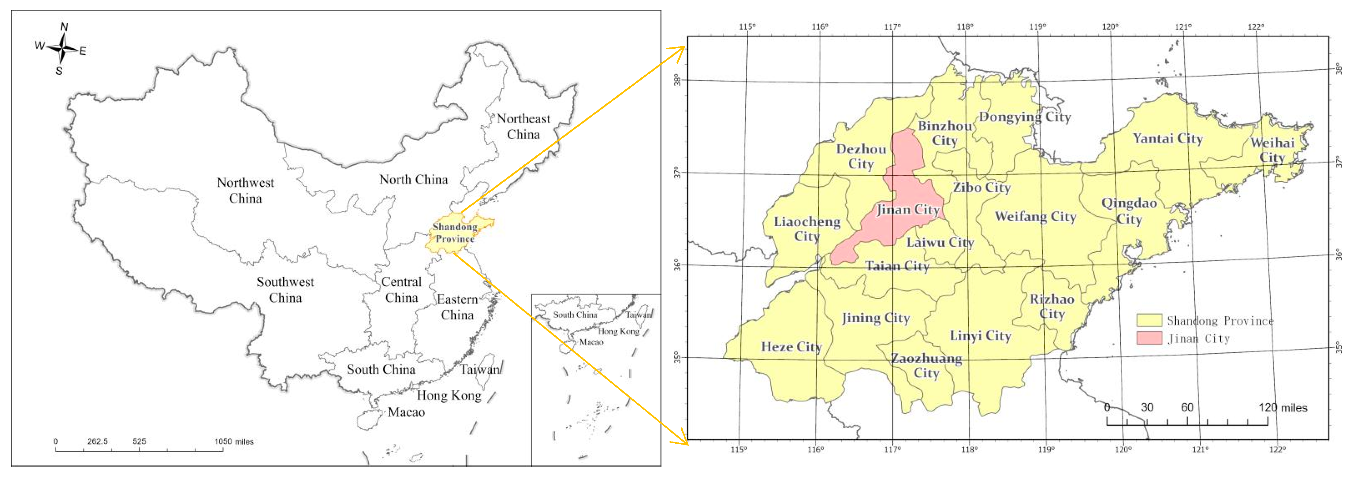
4.1. Overview of the Study Area
4.2. Data Sources
4.3. Results
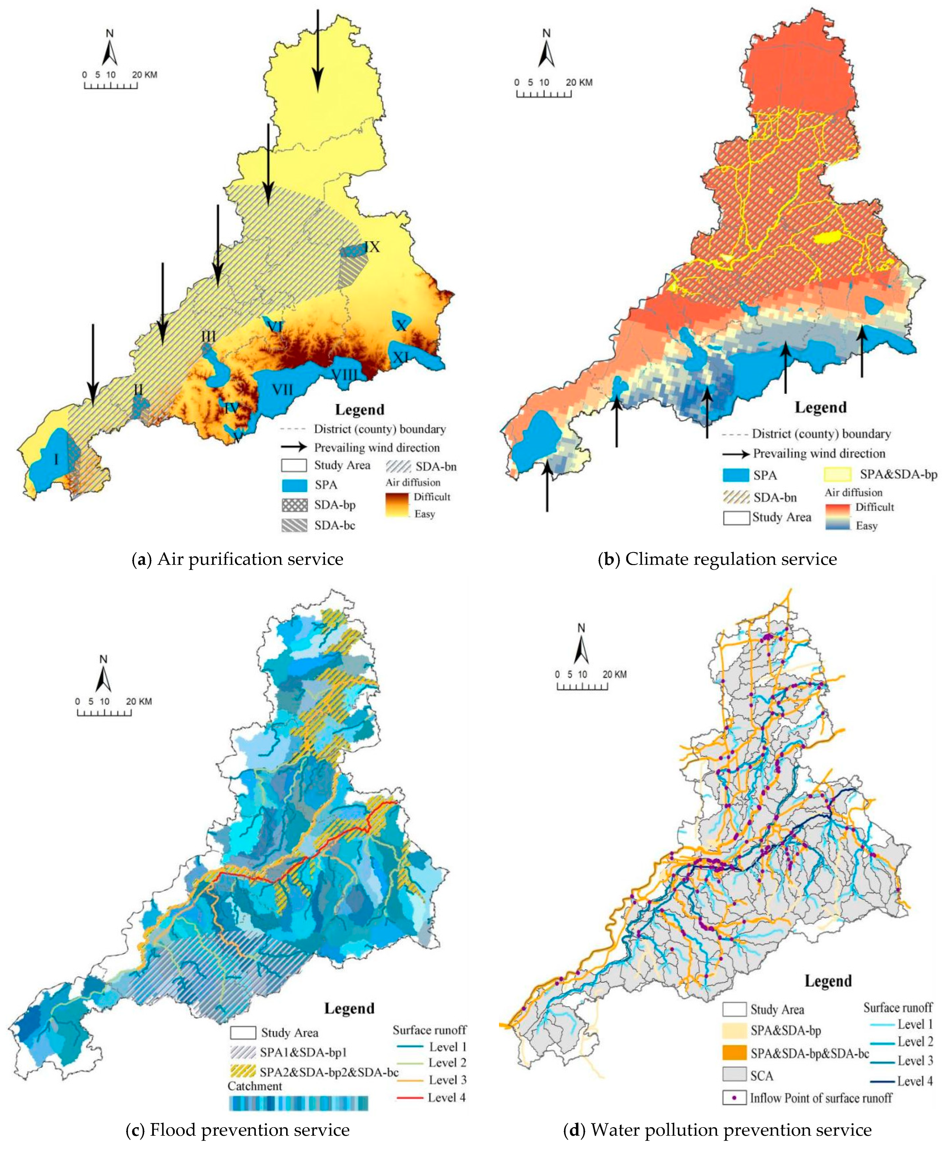
4.3.1. Spatial Distribution Characteristics of Service-Providing, -Connecting and -Demand Areas
- (I)
- Air purification service
- (II)
- Climate regulation service
- (III)
- Flood prevention service
- (IV)
- Water pollution prevention service
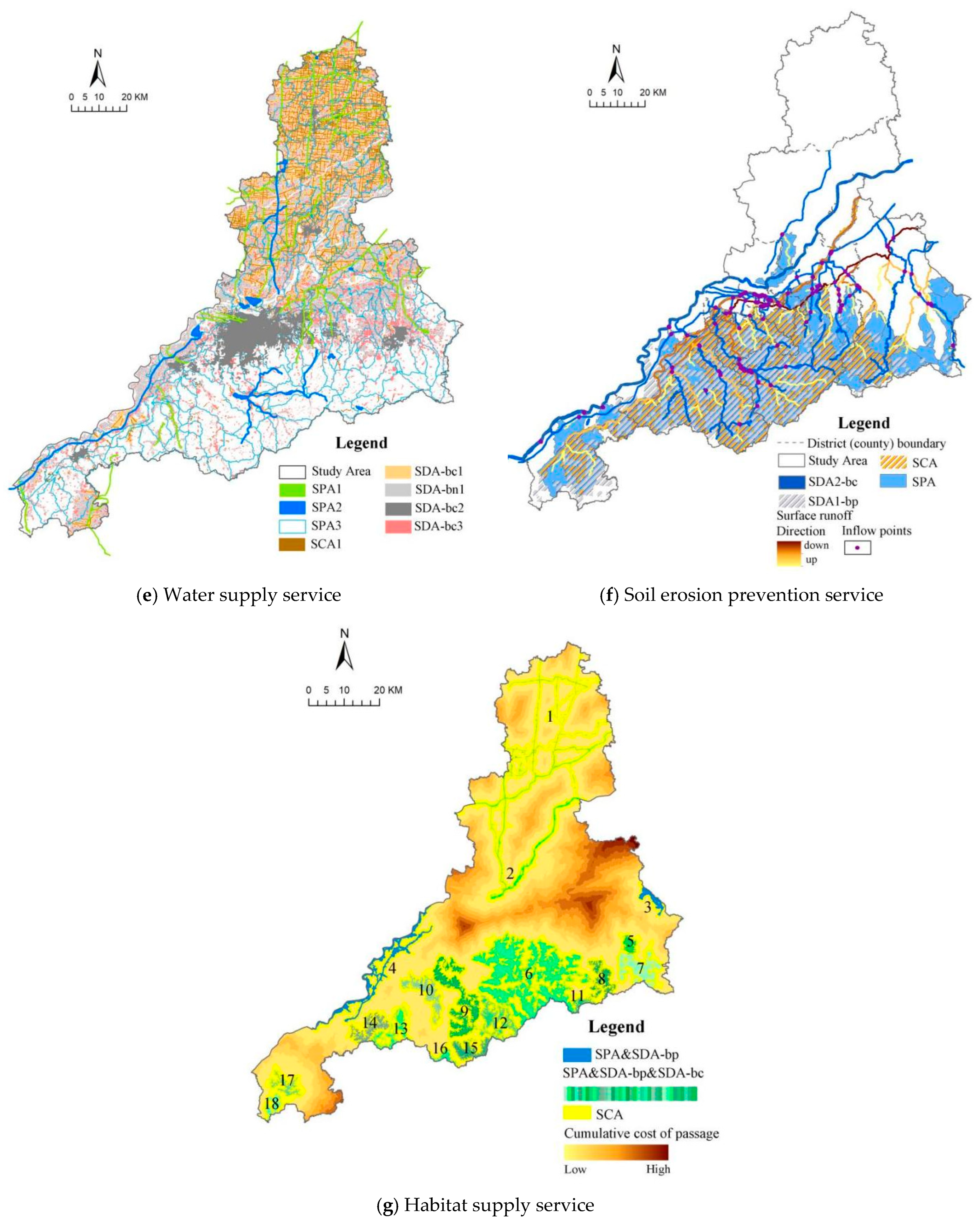
- (V)
- Water supply service
- (VI)
- Soil erosion prevention service
- (VII)
- Habitat supply service
4.3.2. The Impact of Service-Providing and -Connecting Areas on Ecosystem Service Assessment
5. Discussion
- (1)
- Classification of spatial relations among service-providing, -connecting and -demand areas
- (2)
- The key to the improvement of the overall regional ecosystem service provision level
- (1)
- Developing zoning optimization strategies based on the theory of natural geographical differentiation
- (2)
- Identifying and optimizing the main limiting factors of regional service performance based on the short-board effect
- (3)
- The scales of the providing, connecting and demanding areas of ecosystem services
6. Conclusions
Author Contributions
Funding
Institutional Review Board Statement
Informed Consent Statement
Data Availability Statement
Acknowledgments
Conflicts of Interest
References
- Reyers, B.; O’Farrell, P.; Schutyser, F.; Bidoglio, G.; Dhar, U.; Gundimeda, H.; Paracchini, M.L.; Gomez Prieto, O. Measuring biophysical quantities and the use of indicators. In The Economics of Ecosystems and Biodiversity: Ecological and Economic Foundations; Kumar, P., Ed.; Earthscan: London, UK, 2010; pp. 113–148. [Google Scholar]
- Fisher, B.; Turner, R.K.; Burgess, N.D.; Swetnam, R.D.; Green, J.; Green, R.E.; Kajembe, G.; Kulindwa, K.; Lewis, S.L.; Marchant, R.; et al. Measuring, modeling and mapping ecosystem services in the Eastern Arc Mountains of Tanzania. Prog. Phys. Geog. 2011, 35, 595–611. [Google Scholar] [CrossRef]
- Turner, W.R.; Brandon, K.; Brooks, T.M.; Gascon, C.; Gibbs, H.K.; Lawrence, K.S.; Mittermeier, R.A.; Selig, E.R. Global biodiversity conservation and the alleviation of poverty. Bioscience 2012, 62, 85–92. [Google Scholar] [CrossRef]
- Haines-Young, R.; Potschin, M.; Kienast, F. Indicators of ecosystem service potential at European scales: Mapping marginal changes and trade-offs. Ecol. Indic. 2012, 21, 39–53. [Google Scholar] [CrossRef]
- Perrings, C.; Naeem, S.; Ahrestani, F.; Bunker, D.E.; Burkill, P.; Canziani, G.; Elmqvist, T.; Ferrati, R.; Fuhrman, J.A.; Jaksic, F.; et al. Ecosystem services for 2020. Science 2010, 330, 323–324. [Google Scholar]
- Bagstad, K.J.; Johnson, G.W.; Voigt, B.; Villa, F. Spatial dynamics of ecosystem service flow: A comprehensive approach to quantifying actual services. Ecosyst. Serv. 2013, 4, 117–125. [Google Scholar] [CrossRef]
- Serna-Chavez, H.M.; Schulp, C.J.E.; van Bodegom, P.M.; Bouten, W.; Verburg, P.H.; David, M.D. A quantitative framework for assessing spatial flows of ecosystem services. Ecol. Indic. 2014, 39, 24–33. [Google Scholar] [CrossRef] [Green Version]
- Silvestri, S.; Kershaw, F. (Eds.) Framing the Flow: Innovative Approaches to Understand, Protect and Value Ecosystem Services across Linked Habitats; UNEP World Conservation Monitoring Centre: Cambridge, UK, 2010. [Google Scholar]
- Bastian, O.; Grunewald, K.; Syrbe, R.-U. Space and time aspects of ecosystem services, using the example of the EU Water Framework Directive. Int. J. Biodivers. Sci. Ecosyst. Serv. Manag. 2012, 8, 5–16. [Google Scholar] [CrossRef] [Green Version]
- Syrbe, R.-U.; Walz, U. Spatial indicators for the assessment of ecosystem services: Providing, benefiting and connecting areas and landscape metrics. Ecol. Indic. 2012, 21, 80–88. [Google Scholar] [CrossRef]
- Hoekstra, A.; Hung, P. Globalisation of water resources: International virtual water flows in relation to crop trade. Glob. Environ. Change 2005, 15, 45–56. [Google Scholar] [CrossRef]
- Deutsch, L.; Graslund, S.; Folke, C.; Troell, M.; Huitric, M.; Kautsky, N.; Lebel, L. Feeding aquaculture growth through globalization: Exploitation of marine ecosystems for fishmeal. Glob. Environ. Chang. 2007, 17, 238–249. [Google Scholar] [CrossRef]
- Kastner, T.; Erb, K.-H.; Nonhebel, S. International wood trade and forest change: A global analysis. Glob. Environ. Chang. 2011, 21, 947–956. [Google Scholar] [CrossRef]
- Costanza, R. Ecosystem Services: Multiple Classification Systems are Needed. Biol. Conserv. 2008, 141, 350–352. [Google Scholar] [CrossRef]
- Fisher, B.; Turner, R.K.; Morling, P. Defining and Classifying Ecosystem Services for Decision Making. Ecol. Econ. 2009, 68, 643–653. [Google Scholar] [CrossRef] [Green Version]
- Burkhard, B.; Kroll, F.; Nedkov, S.; Mueller, F. Mapping ecosystem service supply, demand and budgets. Ecol. Indic. 2012, 21, 17–29. [Google Scholar] [CrossRef]
- Palomo, I.; Martín-López, B.; Potschin, M.; Haines-Young, R.; Montes, C. National Parks, buffer zones and surrounding lands: Mapping ecosystem service flows. Ecosyst. Serv. 2012, 4, 104–116. [Google Scholar] [CrossRef]
- Marks, R.; Müller, M.J.; Leser, H. Anleitung zur Bewertung des Leistungsvermögens des Landschaftshaushaltes; Zentralausschuß für Deutsche Landeskunde, Selbstverlag: Trier, Germany, 1992. [Google Scholar]
- Röder, M. Mittlere jährliche Gebietsabflusshöhe, Bestimmung von Landschaftsfunktionen und Naturraumpotentialen: Grundlagen, Methoden und exemplarische Ergebnisse, Grundwasserschutzfunktion, Abflussbereitschaft und Regulationsfunklion, Grundwasserneubildung; Forschungen zur deutschen Landeskunde: Flensburg, Germany, 2002. [Google Scholar]
- Nelson, E.J.; Mendoza, G.; Regetz, J.; Polasky, S.; Tallis, H.; Cameron, D.R.; Chan, K.M.A.; Daily, G.C.; Goldstein, J.; Kareiva, P.M.; et al. Modeling Multiple Ecosystem Services, Biodiversity Conservation, Commodity Production, and Tradeoffs at Landscape Scales. Front. Ecol. Environ. 2009, 7, 4–11. [Google Scholar] [CrossRef]
- Horn, W. Selbstreinigungsvermögen von Gewässern; Spektrum: Heidelberg, Germany, 1999; pp. 263–266. [Google Scholar]
- Cowling, R.M.; Pressey, R.L.; Sims-Castley, R.; Le Roux, A.; Baard, E.; Burgers, C.J.; Palmer, G. The Expert or the Algorithm? Comparison of Priority Conservation Areas in the Cape Floristic Region Identified by Park Managers and Reserve Selection Software. Biol. Conserv. 2003, 112, 147–167. [Google Scholar] [CrossRef]
- Hoctor, T.S.; Carr, M.H.; Zwick, P.D. Identifying a Linked Reserve System Using a Regional Landscape Approach: The Florida Ecological Network. Biol. Conserv. 2000, 14, 984–1000. [Google Scholar] [CrossRef]
- Syrbe, R.-U. Biotisches Ertragspotential, Widerstandfähigkeit gegen Wassererosion, Erholungspotential (landschaftlicher Erholungswert); Forschungen zur deutschen Landeskunde: Flensburg, Germany, 2002. [Google Scholar]
- EPA. Frequent Questions; EPA: Washington, DC, USA, 2011.
- Bastian, O. Zur ökologischen Bewertung von Habitationsinseln; Beiträge der Martin-Luther-Universität: Wittenberg, Germany, 1991; pp. 219–224. [Google Scholar]
- Hellwig, Z. Toward a System of Quantitative Indicators of Components of Human Resources Development; UNESCO: Paris, France, 1968. [Google Scholar]
- Łopucki, R.; Kiersztyn, A. Urban Green space conservation and management based on biodiversity of terrestrial fauna-a decision support tool. Urban For. Urban Green. 2015, 14, 508–518. [Google Scholar] [CrossRef]
- Qian, X.; Lee, S.; Soto, A.; Chen, G. Regression Model to Predict the Higher Heating Value of Poultry Waste from Proximate Analysis. Resources 2018, 7, 39. [Google Scholar] [CrossRef] [Green Version]
- Yang, L.-Q.; Levine, E.L.; Smith, M.A.; Ispas, D.; Rossi, M.E. Person-environment fit or person plus environment: A meta-analysis of studies using polynomial regression analysis. Hum. Resour. Manag. J. 2008, 18, 311–321. [Google Scholar] [CrossRef]
- Foley, J.; Costa, M.; Delire, C.; Ramankutty, N.; Snyder, P. Green Surprise? How Terrestrial Ecosystems Could Affect Earth’s Climate. Front. EcoL. Environ. 2003, 1, 38–44. [Google Scholar]


| Service Type | SPA | SCA | SDA | Relevant Literatures |
|---|---|---|---|---|
| Air purification | Land-use unit complexes | - | - | Marks et al. (1992) [18] |
| Climate regulation | Natural units | - | - | Röder (2002) [19] |
| Open spaces uphill around a city | Depth contours and slopes around a city | The city downhill | Syrbe (2012) [10] | |
| Flood prevention | Watersheds | - | - | Nelson et al. (2009) [20] |
| Flood-originating area | Built area within the floodplain | Syrbe (2012) [10] | ||
| Natural units | - | - | Röder (2002) [19] | |
| Water pollution prevention | River sections | - | - | Horn (1999) [21] |
| Natural units | - | - | Röder (2002) [19] | |
| Surface water bodies | Water catchment | Housing or recreation area | Syrbe (2012) [10] | |
| Water supply | Watersheds | - | - | Cowling et al. (2003) [22] |
| Groundwater recharge areas | - | - | Hoctor et al. (2000) [23] | |
| Arable and wetland in a groundwater basin | Pollution risk area in that catchment | Built area, irrigated land in the basin | Syrbe (2012) [10] | |
| Erosion prevention | Natural units | - | Natural units | Syrbe (2002) [24] |
| Wood, hedges, groves around and between acre fields | Field edges | Acre fields | Syrbe (2012) [10] | |
| Habitat supply | Watersheds | - | Watersheds | EPA (2011) [25] |
| Biotopes; natural units | - | - | Bastian (1991) [26] | |
| Sub-habitats for foraging, hunting, and hibernating | Ecological networks | Nesting habitats | Syrbe (2012) [10] |
| Serial No. | Service Type | Composition | Identification Principles | Identification Key Points | Identification Methods |
|---|---|---|---|---|---|
| 1 | Air purification | SPA | Services are generated by specific ecosystems that provide services primarily through biogeochemical processes, regulating CO2/O2, O3 and SOx levels. | SPA is mainly aimed at areas with high forest coverage and high ambient air quality standards. | Using Arcgis 10.8 software, 11 ambient air functional zones of class I were directly extracted from the Jinan ambient air functional zoning. |
| SCA | Air diffusion is involved. | SCA is mainly aimed at the range of fresh air transmission affected by wind direction and topography. | The prevailing wind direction in the study area was north. From north to south, the higher the altitude was, the more difficult the air diffusion was. The spatial scope of SCA was determined by spatial analysis with Arcgis 10.8 software. | ||
| SDA | The principle of directness. | SDA is mainly aimed at areas where air pollutants accumulate. | By using Arcgis 10.8 software, the spatial interpolation method was used to extract the distribution areas with high PM 2.5 concentration. | ||
| 2 | Climate regulation | SPA | Services are generated by specific ecosystems and can effectively regulate regional temperatures. | SPA is mainly aimed at areas with high carbon density or a high net carbon sequestration rate or areas where water bodies are located | Arcgis 10.8 software was used to directly extract ambient air functional zones of class I rivers, lakes, reservoirs, inland beaches and marshes with known boundaries in Jinan city. |
| SCA | Regional or global atmospheric circulation processes is involved. | SCA is mainly aimed at the transfer range of moist and cool air affected by three physical factors: wind direction, gravity and temperature difference. | Based on the analysis of the influence of wind direction, slope direction and temperature difference on air flow, the reclassification tool and spatial weighting overlay tool in Arcgis 10.8 software were used to determine the SCA space range. | ||
| SDA | The principle of directness. | SDA is mainly aimed at areas with obvious heat island effects. | By using Arcgis 10.8 software, the regions with high mean annual temperature were extracted by inverse distance weight interpolation (IDW). | ||
| 3 | Flood prevention | SPA | The service-providing area is also the service-demand area, and the vegetation inside participates in the flood storage and detention process. | SPA is mainly aimed at the rainfall areas and low-lying catchment areas. | By using Arcgis 10.8 software, the kriging interpolation method was used to extract areas with high average annual rainfall and flow direction, and flow accumulation and watershed tools were used to extract the highest-grade catchment area. |
| SCA | This relates to the process of the timely, rapid and massive absorption of rainfall within the spatial collection range of surface runoff. | SCA is mainly aimed at the surface runoff flowing through the catchment area. | By using Arcgis 10.8 software, flow direction and flow accumulation, watershed tools were used to generate surface runoff and the corresponding catchment, and the catchment except for the highest-grade catchment was extracted. | ||
| SDA | The principle of directness and potential. | SDA is mainly aimed at areas with heavy rainfall or low-lying land. | By using Arcgis 10.8 software, the kriging interpolation method was used to extract areas with high average annual rainfall, and flow direction, flow accumulation and watershed tools were used to extract the highest-grade catchment area. | ||
| 4 | Water pollution prevention | SPA | Services are generated by specific ecosystems that participate in processes such as the storage and recycling of a certain amount of organic and inorganic waste through dilution, assimilation and chemical recombination. | SPA is mainly aimed at the spatial scope of rivers, lakes, reservoirs and their affiliated wetlands, and the catchment areas associated with various pollution sources. | On the one hand, rivers, lakes, reservoirs and their affiliated wetlands (such as marshes, tidal flats, etc.) were directly extracted by Arcgis 10.8 software. On the other hand, the above catchments and pollution sources were analyzed by overlay tools, and the catchments associated with various pollution sources were extracted. |
| SCA | This relates to the processes of interception, adsorption and the microbial decomposition of heterogeneous nutrients and compounds by plant roots and soil within a catchment area. | SCA is mainly aimed at the surface runoff flows through the spatial extent. | Based on the above catchment identification results, the corresponding catchment area of surface runoff was extracted. | ||
| SDA | The principle of directness. | SDA is mainly aimed at various water bodies. | The Arcgis 10.8 software was used to extract various water bodies from “Water Environmental Function Zoning” in the 13th Five-Year Plan for the Ecological and Environmental Protection of Jinan city. | ||
| 5 | Water supply | SPA | Agricultural irrigation water source and urban and rural domestic water source supply services through participating in the hydrological cycle of water resource filtration, retention and storage. | SPA is mainly aimed at agricultural water source area, drinking water source area and groundwater catchment area. | The agricultural water functional areas and surface drinking water sources were extracted from the 13th Five-Year Plan for the Ecological and Environmental Protection of Jinan by using Arcgis 10.8 software, and the above catchment areas were added. |
| SCA | This relates to the physical process of transporting water resources to areas of demand. | SCA is mainly aimed at the space laying range and accessibility of its internal ditches, water delivery or water intake pipelines. | By using Arcgis 10.8 software, firstly, the above catchment areas were extracted. Secondly, the spatial laying scope of water supply pipeline facilities was identified based on the relevant information of regional infrastructure status. Thirdly, based on remote sensing data, the ditches used for irrigation were extracted directly. | ||
| SDA | The principle of demand. | SDA is mainly aimed at areas of various types of water use | Using Arcgis 10.8 software and based on remote sensing data, irrigated land, paddy field, urban land, and village land were interpreted. | ||
| 6 | Soil erosion prevention | SPA | This relates to the service provided by vegetation cover and root systems within natural units through participating in soil stabilization, stormwater erosion, and the prevention of compaction and erosion of bare soil | SPA is mainly aimed at the catchment area where the area sensitive to soil erosion is located. | Based on the Arcgis 10.8 software platform, four evaluation indexes including rainfall erosivity, soil erodibility, slope and vegetation coverage were selected and weighted. A suitability evaluation method was adopted to comprehensively evaluate the sensitivity to regional soil erosion. Based on the evaluation results, areas that were highly sensitive to soil erosion were extracted and spatially superimposed with the above catchments. Finally, the catchment area where the area sensitive to soil erosion was located was extracted. |
| SCA | This relates to the process in which the vegetation cover and the vegetation root system in the catchment block the surface runoff carrying sediment into the drainage system | SCA is mainly aimed at the surface runoff flows through the space between the catchment where the area sensitive to soil erosion is located and the water system | The catchment space associated with surface runoff was extracted according to the screening principle of surface runoff flowing through the area sensitive to soil erosion, and finally into rivers, reservoirs and natural lakes. | ||
| SDA | The principle of directness and potential | SDA is mainly aimed at areas with a high risk of soil erosion or areas prone to soil erosion disasters | Based on the Arcgis 10.8 software platform, on the one hand, the areas that were highly sensitive to soil erosion were extracted; on the other hand, based on the above surface runoff extraction results, rivers, reservoirs and natural lakes fed by surface runoff flowing through areas that were highly sensitive to soil erosion were extracted. | ||
| 7 | Habitat supply | SPA | Services are generated by specific ecosystems that support the life activities, evolution and reproduction processes of flora and fauna. | SPA is mainly aimed at living areas of flora, fauna and microorganisms. | The region group tool in Arcgis 10.8 was used to merge the forest land, grassland, wetland and natural water body that were spatially related to each other, and extract the large patches with an area of more than 10 km2 after merging. |
| SCA | This relates to the functions of natural units such as breeding, nesting, foraging, reproduction or migration. | SDA is mainly aimed at the ecological corridor or ecological steppingstone and other related land that can connect various ecological sources. | Based on the spatial weighted distance tool in the spatial analysis module of the ArcGIS 10.8 software platform, the space of minimum passage cost between SPA was taken as the result of SCA recognition, representing the possible movement trends, directions and range of animals in the space. | ||
| SDA | The service-providing area is also the service-demand area, | SDA is mainly aimed at the living area of flora, fauna and microorganisms. | The region group tool in Arcgis 10.8 was used to merge the forest land, grassland, wetland and natural water bodies that were spatially related to each other and extract the large patches with an area of more than 10 km2 after merging. |
| Related Index | Related Index Value of SPA | Related Index Value of SCA | Related Index Value of Overall Area |
|---|---|---|---|
| Service diversity index | 7.79 | 5.91 | 11.21 |
| Service diversity participation rate (%) | 39.86 | 34.50 | 68.30 |
| Benefit area rate of service demand area (%) | 65.91 | 54.89 | 94.79 |
| Service benefit contribution rate (%) | 61.86 | 38.14 | 100.00 |
| Shk index | 99.99 | 99.92 | - |
| Service Type | Services in the Case | SDA Benefits from the SPA | SDA Benefits from the SCA |
|---|---|---|---|
| Provision-oriented type (transitive type) | Air purification service; Climate regulation service; Water supply service; Habitat service. |  |  |
| Prevention-oriented type (local type) | Flood prevention service; Water pollution prevention service; Soil erosion prevention service. |  |  |
Publisher’s Note: MDPI stays neutral with regard to jurisdictional claims in published maps and institutional affiliations. |
© 2022 by the authors. Licensee MDPI, Basel, Switzerland. This article is an open access article distributed under the terms and conditions of the Creative Commons Attribution (CC BY) license (https://creativecommons.org/licenses/by/4.0/).
Share and Cite
Liu, Q.; Du, G.; Liu, H. A Quantitative Study on the Identification of Ecosystem Services: Providing and Connecting Areas and Their Impact on Ecosystem Service Assessment. Sustainability 2022, 14, 7904. https://doi.org/10.3390/su14137904
Liu Q, Du G, Liu H. A Quantitative Study on the Identification of Ecosystem Services: Providing and Connecting Areas and Their Impact on Ecosystem Service Assessment. Sustainability. 2022; 14(13):7904. https://doi.org/10.3390/su14137904
Chicago/Turabian StyleLiu, Qing, Guoming Du, and Haijiao Liu. 2022. "A Quantitative Study on the Identification of Ecosystem Services: Providing and Connecting Areas and Their Impact on Ecosystem Service Assessment" Sustainability 14, no. 13: 7904. https://doi.org/10.3390/su14137904