Article

Numerical Simulation of the Liquefaction Phenomenon by MPSM-DEM Coupled CAES

1
Graduate School of Engineering and Science, Shibaura Institute of Technology, Tokyo 135-8548, Japan
2
College of Engineering, Shibaura Institute of Technology, Tokyo 135-8548, Japan
3
Aomi Construction Co., Ltd., Tokyo 101-0021, Japan
4
Department of Civil Engineering, Kasetsart University, Bangkok 10900, Thailand
*
Author to whom correspondence should be addressed.
Sustainability 2022, 14(12), 7517; https://doi.org/10.3390/su14127517
Submission received: 6 May 2022 / Revised: 13 June 2022 / Accepted: 17 June 2022 / Published: 20 June 2022

Abstract

:
The mechanism of liquefaction and the factors that cause liquefaction behavior have previously been examined and evaluated, both analytically and experimentally; construction including liquefaction countermeasures is being implemented, based on these findings. This study presents a theoretical visualization of the mechanism of liquefaction generation and evaluates the behavior of particles in the ground. Specifically, an MPSM-DEM coupled CAE system (CAES) is employed to view the events beneath the ground, modeled three-dimensionally when an external acceleration is applied to simulate seismic waves and reveals the behavior below the surface. The numerical simulation of the liquefaction phenomenon, as represented by an MPSM-DEM coupled CAES system, clearly showed the mechanism of liquefaction generation and contributed to the design and accountability of more economical and sustainable liquefaction countermeasures, regardless of the field of specialization.

1. Introduction

With the 1964 Niigata earthquake and studies on liquefaction being energetically pursued, the conditions under which the ground will easily liquefy were clarified. However, the damage caused by liquefaction due to the 2011 earthquake off the Pacific coast of East Japan extended to the Kanto region, and the metropolitan area also suffered great damage [1,2,3]. Although the mechanism of liquefaction and the factors that cause liquefaction had previously been examined and evaluated, both analytically and experimentally [4,5,6,7,8,9,10,11], and despite the fact that construction countermeasures related to liquefaction had been implemented based on those earlier findings, the liquefaction damage during the 2011 earthquake off the Pacific coast of East Japan was enormous. One of the reasons for the scale of destruction is that there were no cases in which the effects of the liquefaction countermeasures had been visually examined and evaluated. As Japan has a large number of areas with soft ground composed of fine particles such as sand, and it lies in an area where several continental and oceanic plates meet, earthquakes frequently occur. Therefore, in order to prevent further damage caused by liquefaction in these areas, efficient and economical liquefaction measures are indispensable.
Based on the above background, the mechanism of liquefaction generation is visualized theoretically in this study, using a coupled computer-aided engineering system (CAES), the moving particle semi-implicit method (MPSM), and the discrete element method (DEM) [12,13]. CAES is a general term for technology that includes using a computer to simulate and analyze prototypes created using computer-aided design (CAD), considering the site conditions. The CAES in this study is executed using an algorithm in which the MPSM and DEM methods are combined.
In this study, external acceleration, simulating seismic waves, is applied to a ground surface modeled three-dimensionally using the coupled CAES of the MPSM and the DEM, for the purposes of revealing the behavior of the particles in the modeled ground and examining whether liquefaction is likely to occur in it. By visualizing the liquefaction phenomenon, it is expected that the mechanism of liquefaction generation will be clearly shown and that this will contribute to the development and accountability of more efficient and economical liquefaction countermeasures. By utilizing CAES to recreate the phenomenon of liquefaction, it is possible to visualize the generating mechanism of liquefaction, which cannot normally be seen in the natural ground, and solve the complicated problems associated with its manifestation [12,13]. In addition, since design and evaluation can be performed while comparing and examining the models of various ground conditions, it is thought that the design quality can be improved at an early stage and that a more effective construction method can be designed.

2. Background of the Analysis of Liquefaction

Since the 1964 Niigata earthquake and the 1995 Great Hanshin-Awaji earthquake, studies on liquefaction in the region have increased and research has actively been conducted [1,2,14]. Thanks to these studies, understanding, predicting, and establishing countermeasure technologies for liquefaction have almost been achieved. Liquefaction during an earthquake is a phenomenon in which a saturated sandy soil is repeatedly subjected to shear stress; the shear rigidity decreases as the effective stress decreases, and finally, the shear resistance is lost, and the soil behaves like a viscous fluid. Therefore, in order to simulate and analyze the mechanical behavior of soil during liquefaction, the process of the change from solid to fluid must be considered.
Effective stress analysis is one of the typical methods used for analyzing ground deformation during liquefaction [15,16]. An effective stress analysis incorporates the constitutive law of sand into the equation for the field in which the soil skeleton and the pore water are coupled, which is obtained based on solid dynamics. The effective stress analysis covers the initial state of the ground, the dynamic behavior of the ground during an earthquake, and the occurrence of liquefaction. Thus far, many constitutive equations for sand have been proposed, based on solid-state mechanics, according to the results of laboratory tests on the repeated shear behavior of sand [17,18]. These constitutive equations for sand can reproduce the stress-strain relationships and its dilatancy behavior under various stress conditions. As part of the constitutive equations for sand, a repetitive elastoplastic model, an elastoplastic under-load surface model, a densification model, and so on, have been proposed. Conversely, analysis methods that target only the flow process after liquefaction has occurred have also been proposed; these can be divided into methods based on solid-state mechanics and methods based on fluid mechanics. As a method based on solid-state mechanics, for example, Yasuda et al. [19,20] proposed a residual deformation analysis method that can analyze the flow associated with liquefaction with simplicity and practical accuracy. As a method based on fluid mechanics, for example, Uzuoka et al. [21] proposed a method to analyze liquefied sand as a Bingham fluid, and quantitatively showed the flow force and large deformation after the flow, although under relatively simple boundary conditions.
The above-mentioned analysis methods were proposed, paying attention to either the solid or the fluid property of the liquefied sand; however, they did not consider a fusion of the two properties. In the actual liquefaction phenomenon, the phase change process between solid and fluid is considered to occur non-uniformly, both spatially and temporally. At a certain time, the regions having solid and fluid properties become mixed. In order to deal with such problems, it is necessary to develop a simulation method that can express the regions of transition between solid and fluid states.
In this study, the authors propose a CAES that combines the MPSM, as one of the typical particle-based methods (PBMs), and the DEM in an analysis model that can express the phase change process during liquefaction. This is demonstrated in a combination of sand particles in the target ground that are simulated and analyzed by the DEM, and the pore water, simulated and analyzed by the MPSM. A simulation will be performed using this method to examine the effectiveness of the simulation model.

3. MPSM-DEM Coupled CAES

3.1. Computer-Aided Engineering System (CAES)

A computer-aided engineering system (CAES) is a type of alternative technology for running large-scale experiments, conducted in a room or in situ, using prototypes that have been prepared for a study as part of the development process of “manufacturing”. In other words, CAES is a general term incorporating technology that simulates and analyzes prototypes on a computer created using computer-aided design (CAD), considering the site conditions [22,23,24,25]. At the same time, CAES may refer to computer-aided engineering work or its tools for the prior examination, design, manufacturing, and process design of construction methods and products. In the field of geotechnical engineering, CAES can be used not only to visualize beneath the surface of the ground and the stress loading inside the ground but also to estimate the results of experiments that would otherwise involve huge expense, and/or phenomena that would be difficult to reproduce. In addition, by performing the appropriate post-processing, it is possible to communicate the results to other people in a visually accessible manner.
In this study, external acceleration simulating seismic waves is applied to a ground model, created three-dimensionally via the coupled CAES of the moving particle semi-implicit method (MPSM), one of the typical particle-based methods (PBMs), and the discrete element method (DEM), wherein the particles in the modeled ground are subjected to loading. The purpose is to clarify the behavior.

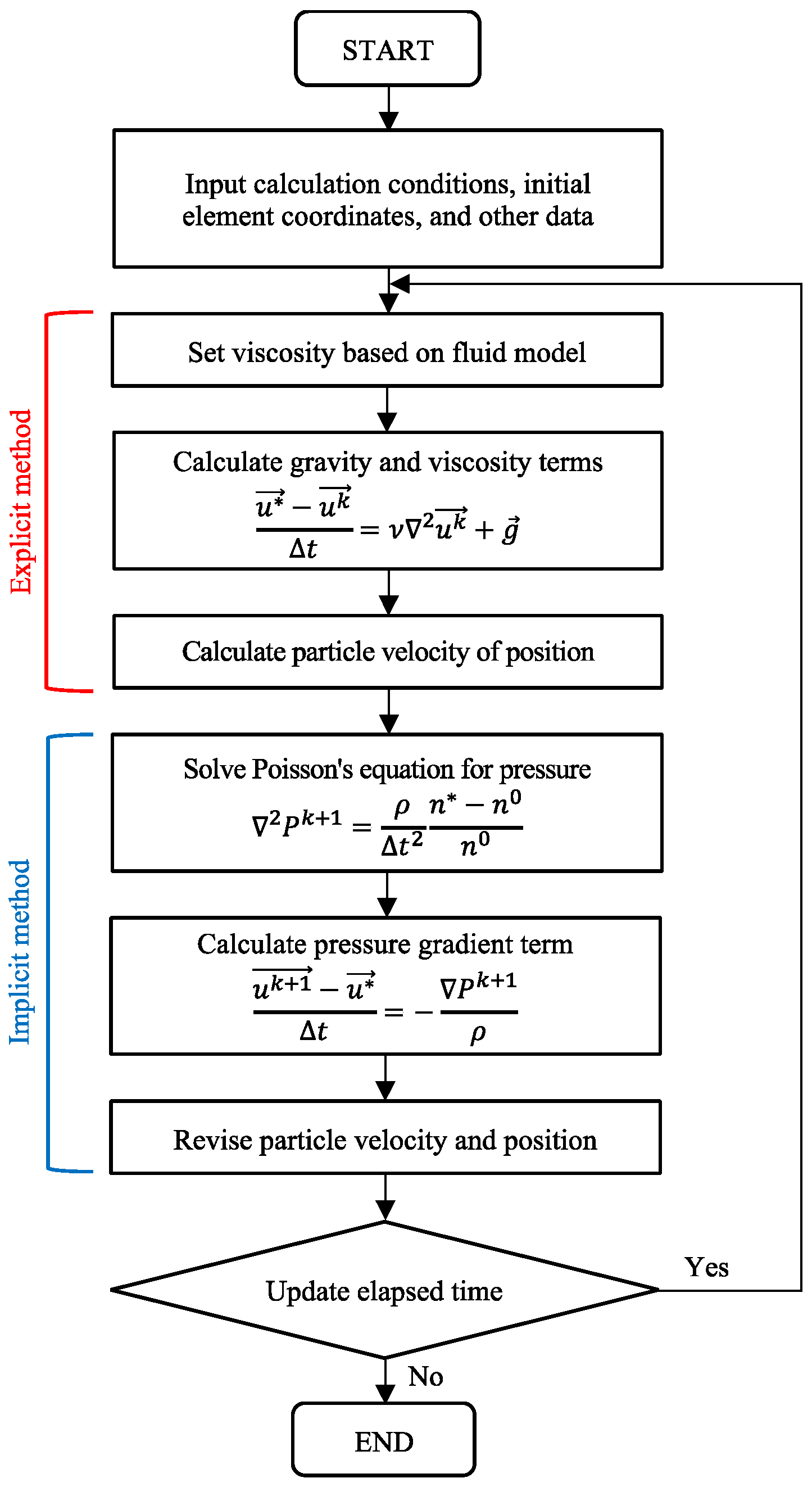
3.2. Particle-Based Method (PBM) and Moving Particle Semi-Implicit Method (MPSM)

A major feature of particle-based methods (PBMs) is that, unlike the finite element method (FEM) and the finite difference method (FDM), they do not use a lattice, but instead discretize the continuum as particles that move each calculation point with a physical quantity. However, this makes a substantial difference to the governing equation. To describe the behavior of a continuum, the Euler method (with a lattice: FEM, FDM, and so on) and the Lagrange method (the non-grid PBM) are available. In the Lagrange method, the calculation point moves as the object moves and deforms, so the convection term disappears from the governing equation. Equations (1) and (2) show the Navier–Stokes equations using the Euler method and the Lagrange method, respectively [26,27,28,29,30]:
u ( x , t ) t + ( u ( x , t ) · ) u ( x , t ) = 1 ρ P ( x , t ) + υ 2 u ( x , t ) + g ( x , t )
D u ( X , t ) D t = 1 ρ P ( x , t ) + υ 2 u ( X , t ) + g ( X , t )
where u is the velocity, P is the pressure, g is the external force, ρ is the density, and υ is the kinematic viscosity coefficient.
The moving particle semi-implicit method (MPSM), one of the typical PBMs, is an incompressible flow analysis method that discretizes a continuum with particles. The basic governing equations are the continuity equation, shown as Equation (3), and the Navier–Stokes equation, shown as Equation (4):
D ρ D t = 0
D u D t = P ρ + ν 2 u + g
where D / D t represents the Lagrange derivative, ρ is the density, u is the velocity, P is the pressure, ν is the coefficient of kinematic viscosity, and g is the gravity. In PBMs, the Navier–Stokes equation is divided into two steps; the pressure term is calculated explicitly from Equation (5) and the pressure gradient term is calculated implicitly from Equations (6) and (7):
u * u k t = ν 2 u k + g
2 P k + 1 = ρ t 2 n * n 0 n 0
u k + 1 u * t = P k + 1 ρ
where n is the particle number density (a dimensionless quantity representing the density of the particle arrangement), n 0 is the standard particle number density, and k is the time step. Here, * indicates a physical quantity at the stage when the explicit calculation has been completed. Figure 1 shows the calculation algorithm of the MPSM.

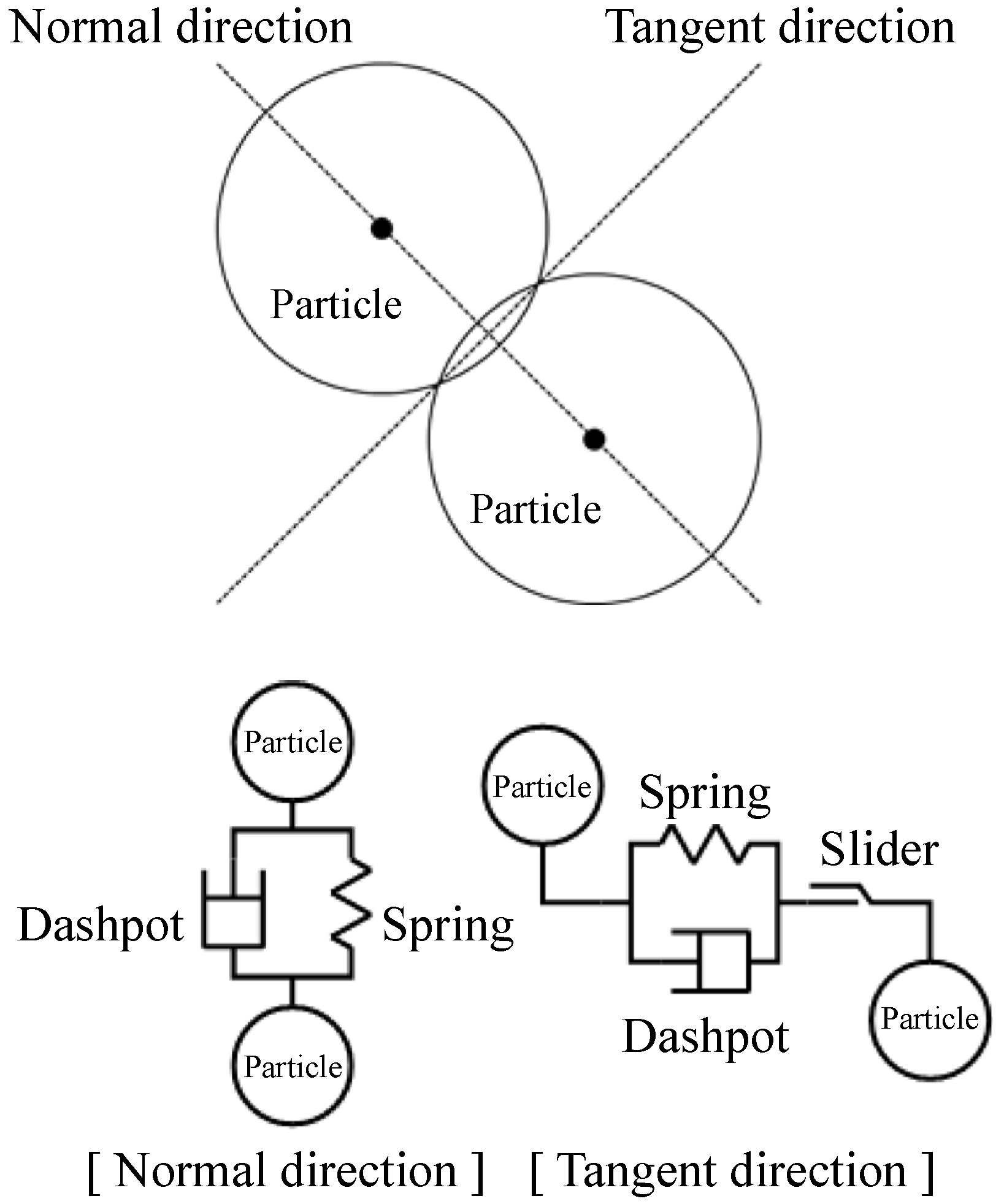
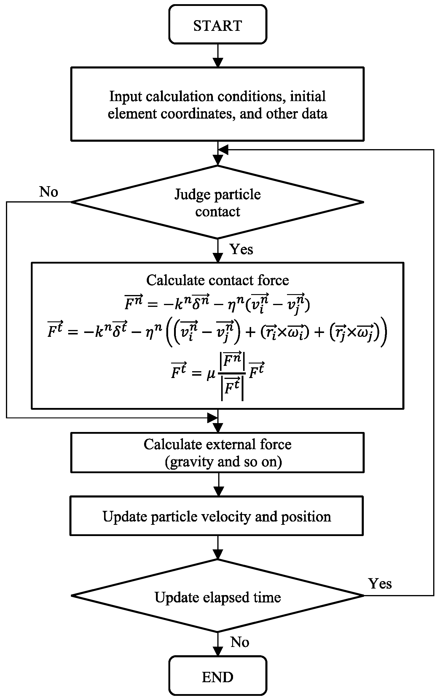
3.3. Discrete Element Method (DEM)

The discrete element method (DEM) is an analysis method proposed by Cundall [31,32]. It considers the analysis target as a collection of minute particles and analyzes the motion of each particle, in order to determine the behavior and reaction force of the entire aggregate [31,32]. The DEM is based on a discontinuum model, unlike the FEM and the PBM, which are based on continuum mechanics. The elements used in the calculation are represented as rigid bodies that do not deform and have a finite size. In addition, a contact force acts when the elements come into contact with each other, and the behavior of an aggregate of discontinuums can be expressed by solving the motion of each element, based on the contact force. Polygonal elements were used in Cundall [31,32], but as they were applied in various fields, spherical elements became popular because of their simple contact algorithm. The individual element method models the object of the analysis as a set of polygons, circles (2D), and spheres (3D) that can move freely, and does the same for each individual element in the set of elements, separated by discontinuities. The behavior of the elements is tracked by establishing an independent second-order ordinary differential equation, approximating the difference, placing it in the time domain, and solving it step by step. Solving the dynamic behavior of each element results in a solution reflecting the aggregates for each element. The DEM then evaluates the dynamic behavior and deformation of the aggregates of each element.
The discrete element method (DEM) is a method of analyzing the behavior of powder by following individual particles, according to the equations of motion. The equations of motion for translational motion and rotational motion are shown in Equations (8) and (9), respectively:
m d d t v = F
I d d t ω = M
where m is the mass, v is the velocity, F is the force, I is the moment of inertia, ω is the angular velocity, and M is the rotational moment. In the case of spherical particles, the moment of inertia is expressed by Equation (10):
I = 2 5 m r 2
where r is the radius of the spherical particles. In the DEM, the particles are treated as rigid particles that do not deform, and overlapping between particles is allowed. The contact force of the particles (repulsive force, energy damping, and slip due to friction) is expressed by the spring model, viscous damping model, and slider model, as shown in Figure 2, respectively, and the magnitude of the contact force is expressed by Equations (11) and (12):
F n = k n δ n η n ( v i n v j n )
F t = k t δ t η t ( ( v i n v j n ) + ( r i × ω i ) + ( r j × ω j ) )
where k is the spring constant, δ is the amount of overlap, η is the damping coefficient, v is the velocity, r is the distance from the particle’s center of gravity to the contact point, and ω is the angular velocity. Superscript n represents the normal component, t represents the tangential component, and subscripts i and j represent each particle. Moreover, when the ratio of the tangential and normal components of the contact force exceeds the friction coefficient, μ , the particles undergo slippage, as modeled by the slider model. The contact force in the tangential direction at that time is replaced by Equation (13).
F t = μ | F n | | F t | F t
The calculation algorithm for the DEM is shown in Figure 3.

3.4. MPSM-DEM Coupled CAES

In the MPSM-DEM coupled system, the equations expressing the motion of the fluid and the powder are given as Equations (14) and (15), respectively. For the sake of simplicity, it is assumed here that there is no external force:
ρ D ε v l D t = ε P + ν 2 ε v l ε l 0 3 F D
m D v s D t = F D E M + F D + F P
where ρ is the density of the fluid, ε is the body integration factor of the fluid, v l is the velocity of the fluid, P is the pressure of the fluid, ν is the kinematic viscosity coefficient of the fluid, m is the mass of the powder, v s is the velocity of the powder, F D E M is the contact force by the DEM, F D is the fluid resistance, and F P is the buoyancy. The fluid resistance and buoyancy are expressed by Equations (16) and (17), respectively:
F D = π 2 C d ρ r 2 ε 2 χ | v l v s | ( v l v s )
F P = V s P
where C d is the fluid resistance coefficient (defined as a function of the Reynolds number R e ), r is the particle radius of the powder, and v s is the particle volume of the powder. Here, χ is expressed by Equation (18):
χ = 3.7 0.65 exp ( ( 1.5 l o g R e ) 2 2 )
R e = 2 r ε | v l v s | ν
where ν is the coefficient of kinematic viscosity for the fluid.

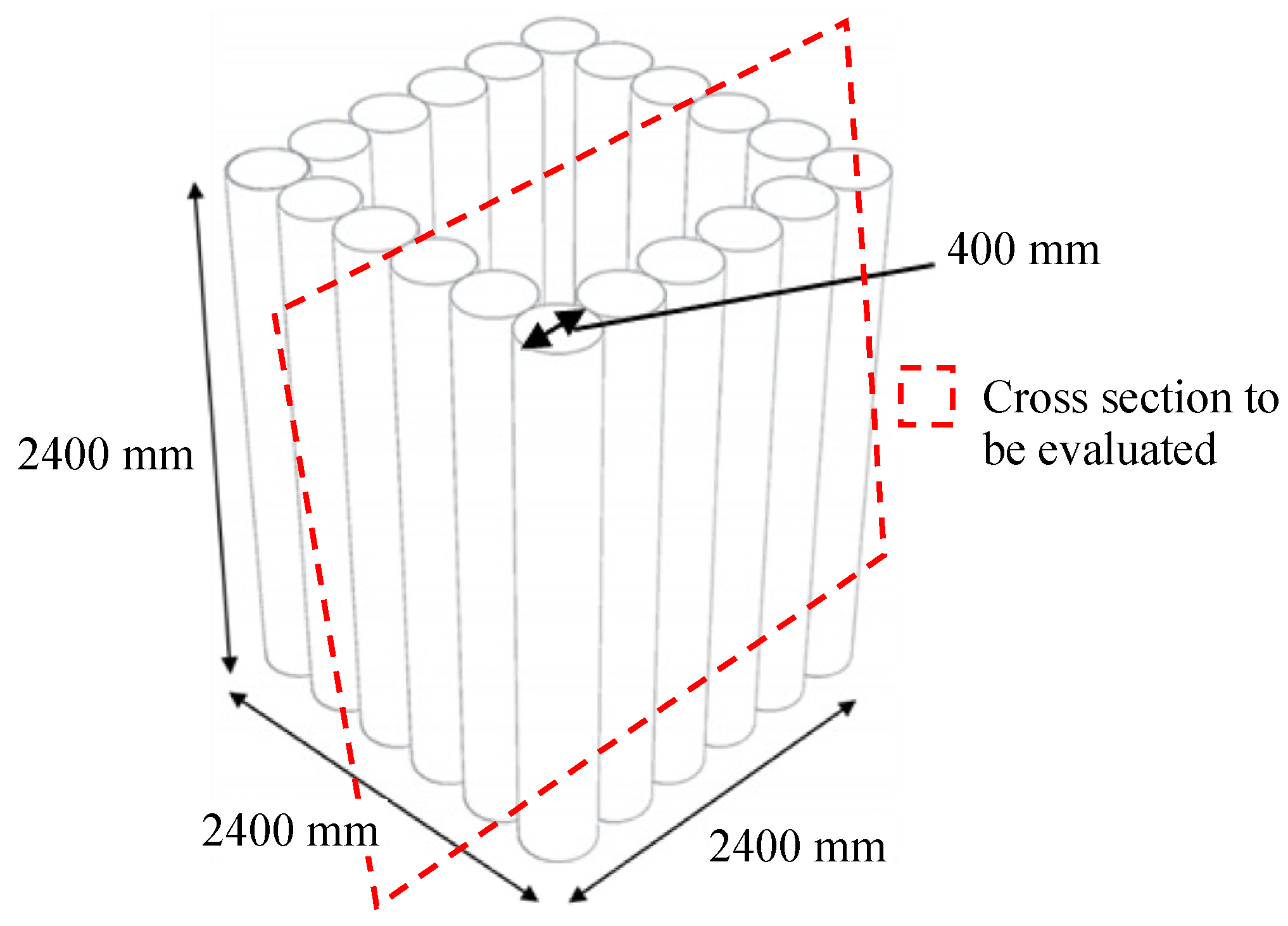
4. Simulation Model and Conditions

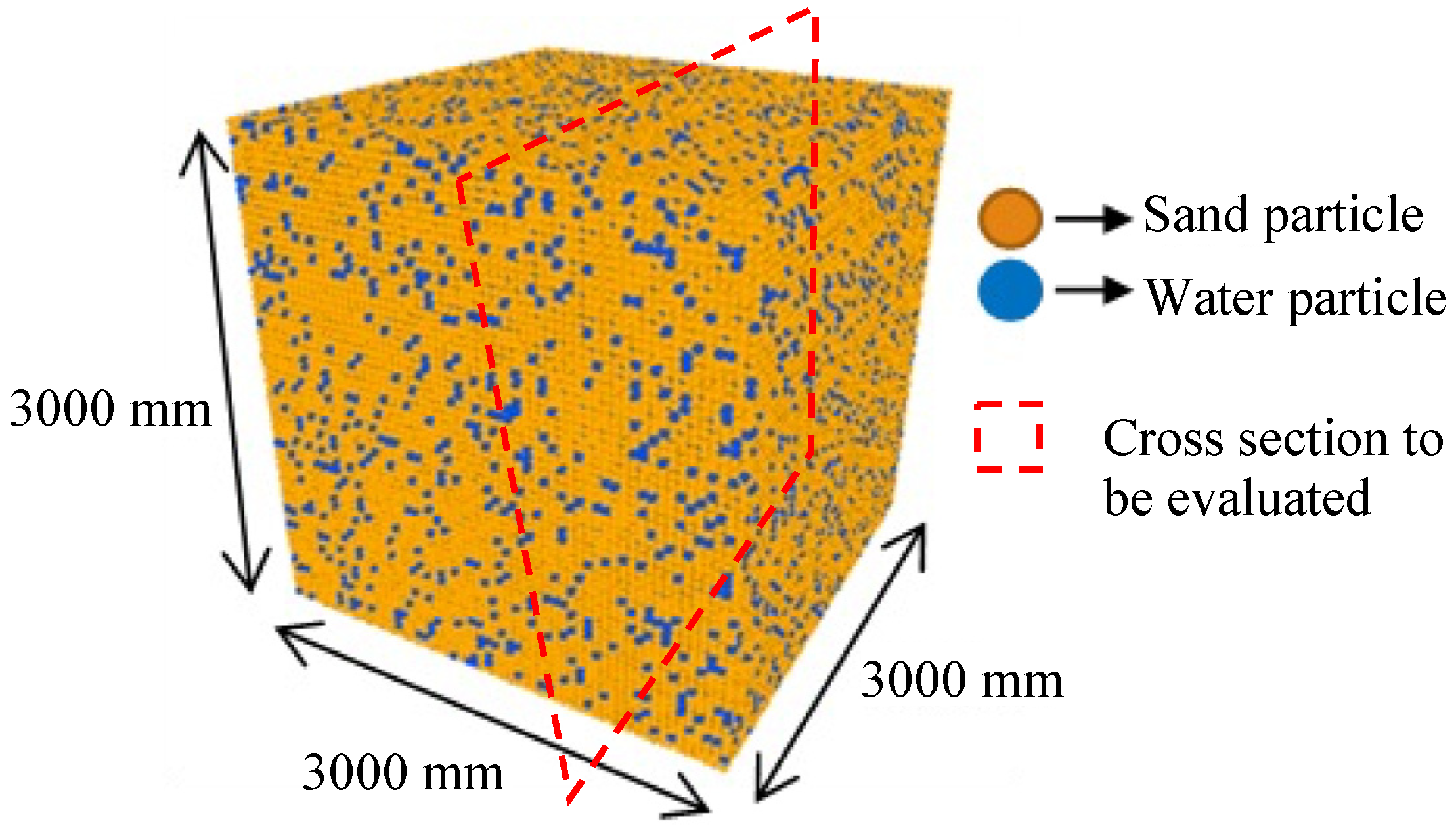
4.1. Simulation Model

The analytical model is shown in Figure 4. The sand particles and water particles are arranged according to the void ratio on a 3000 mm-square cube. The sand particles are displayed in yellow, and the water particles are displayed in blue, to visually express the ground surface. In addition, a ground model simulating the liquefaction countermeasures is reproduced. This is used as the pile model and is shown in Figure 5. The piles are 400 mm in diameter and 3000 mm in length, and six piles are arranged on each of the four sides. The piles are placed on the ground model, as shown in Figure 5, and the simulation is performed as shown in Figure 4 and Figure 5.

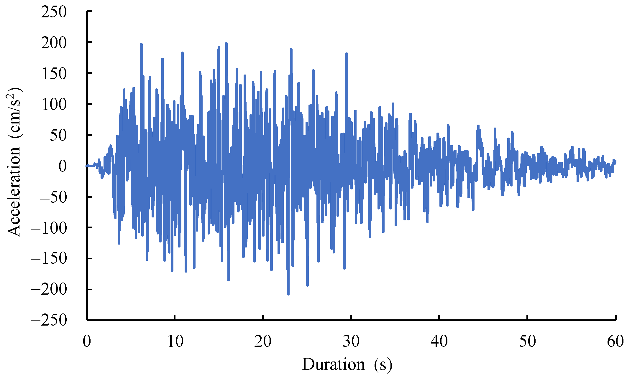
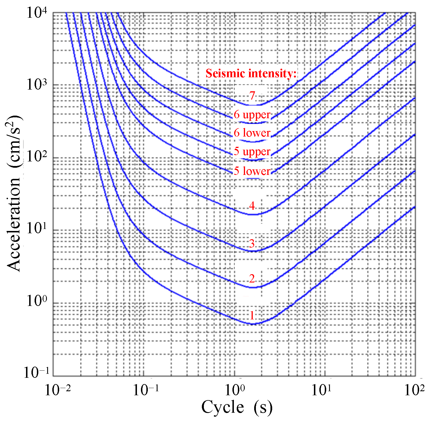
4.2. Setting of External Acceleration

In this study, liquefaction is brought about by applying an external acceleration to the ground model that simulates seismic waves. Figure 6 shows the assumed parameters of the external acceleration, using data published by The Building Center of Japan [33]. Acceleration is given in the X-axis direction every 0.01 s for a total of 59.99 s. Figure 7 shows the relationship between acceleration and seismic intensity [34]. The maximum value of acceleration is adopted as a parameter representing seismic intensity. The maximum value of the external acceleration parameter is 207.33 (cm/s2), which corresponds to an earthquake with a seismic intensity of 5 or higher, as shown in Figure 7. The reason for setting this seismic intensity is that the liquefaction phenomenon often occurs from an earthquake that has a seismic intensity of 5 or higher.
Figure 4. Cross-section of Cases 1 and 2, targeted for analysis (without liquefaction measures).
Sustainability 14 07517 g004
Figure 5. Cross-section of Case 3, targeted for analysis (characteristic display of a liquefaction countermeasure part by grid-shaped piles).
Sustainability 14 07517 g005

4.3. MPSM-DEM Coupled CAES Settings

In this study, water was set as a fluid by the MPSM, and the sand was set as powder particles by the DEM. Table 1 shows the physical characteristics of the water particles modeled by the MPSM, while Table 2 shows the physical characteristics of the sand particles modeled by the DEM. The MPSM parameters of water can be established by referring to the physical characteristics of water at a temperature of 20 °C [35], and the DEM parameters of the sand particles can be found by referring to the parameters used in previous studies [12,13,24,28,30,36,37]. Considering the time required for the calculation, the distance between the particles in the MPSM was set at 20 mm, and the particle size in the DEM was set at 20 mm. Attention should be paid to the DEM parameters for the sand particles shown in Table 2, particularly when setting the sand particle’s diameter and density. The typical sand particle diameter and density are 0.2 mm and 2.634 g/cm3, respectively. In this study, the diameter and density of the sand particles modeled by the DEM were set so that the particle sedimentation velocity of the Stokes fluid [38,39] was equal to that of typical sand particles and the sand particles modeled by the DEM. In this paper, the authors focus on the void ratio and express the sandy ground via the void ratio, using the maximum and minimum void ratios of a typical sandy ground. The void ratios for three case studies are shown in Table 3. The void ratio for Case 1 is 1.19, that for Case 2 is 0.71, and that for Case 3, with the piles, is 1.19.
Figure 6. Time history of the external acceleration applied in the analysis.
Sustainability 14 07517 g006
Figure 7. Relationship between period, acceleration, and seismic intensity (theoretical value).
Sustainability 14 07517 g007

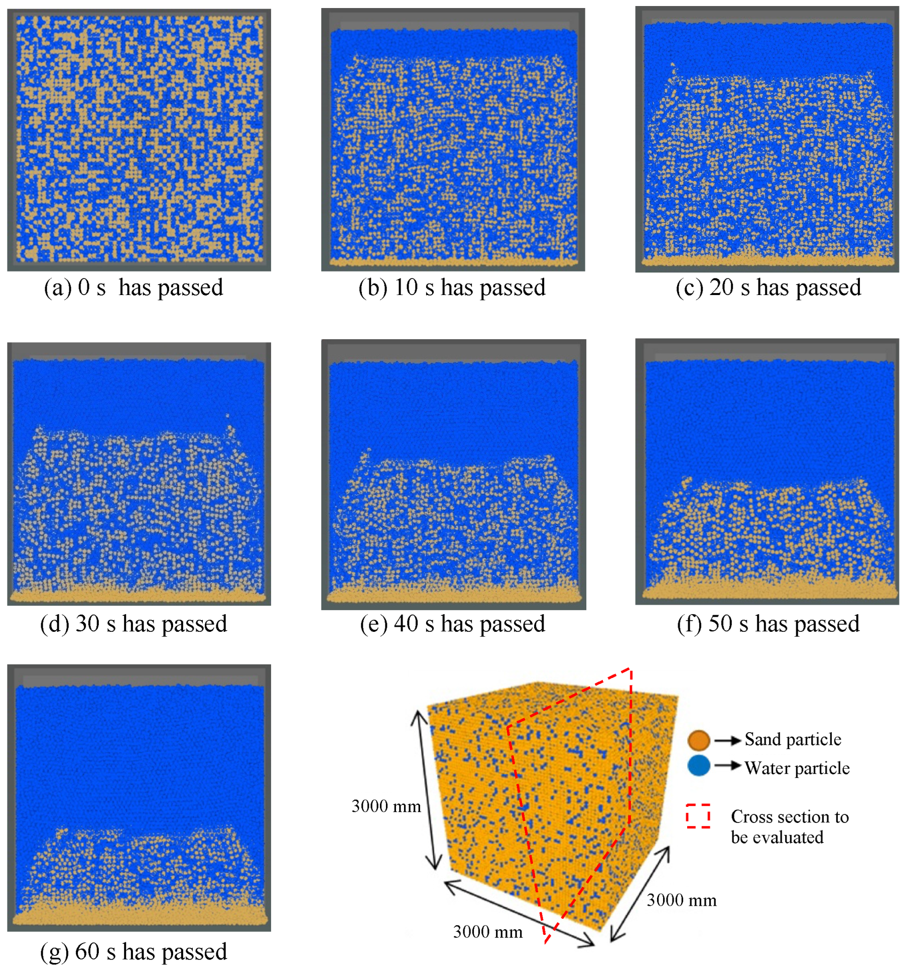
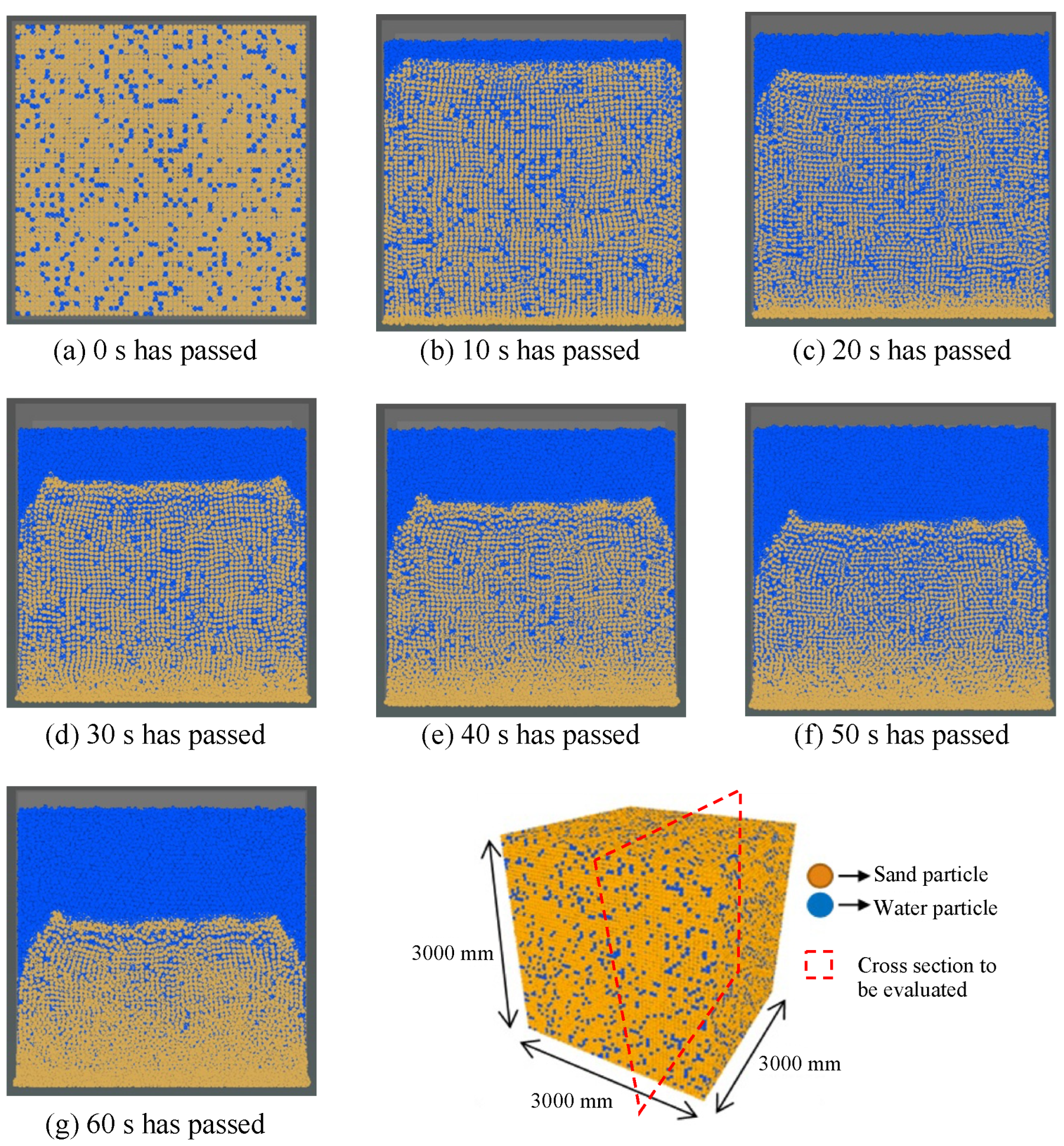
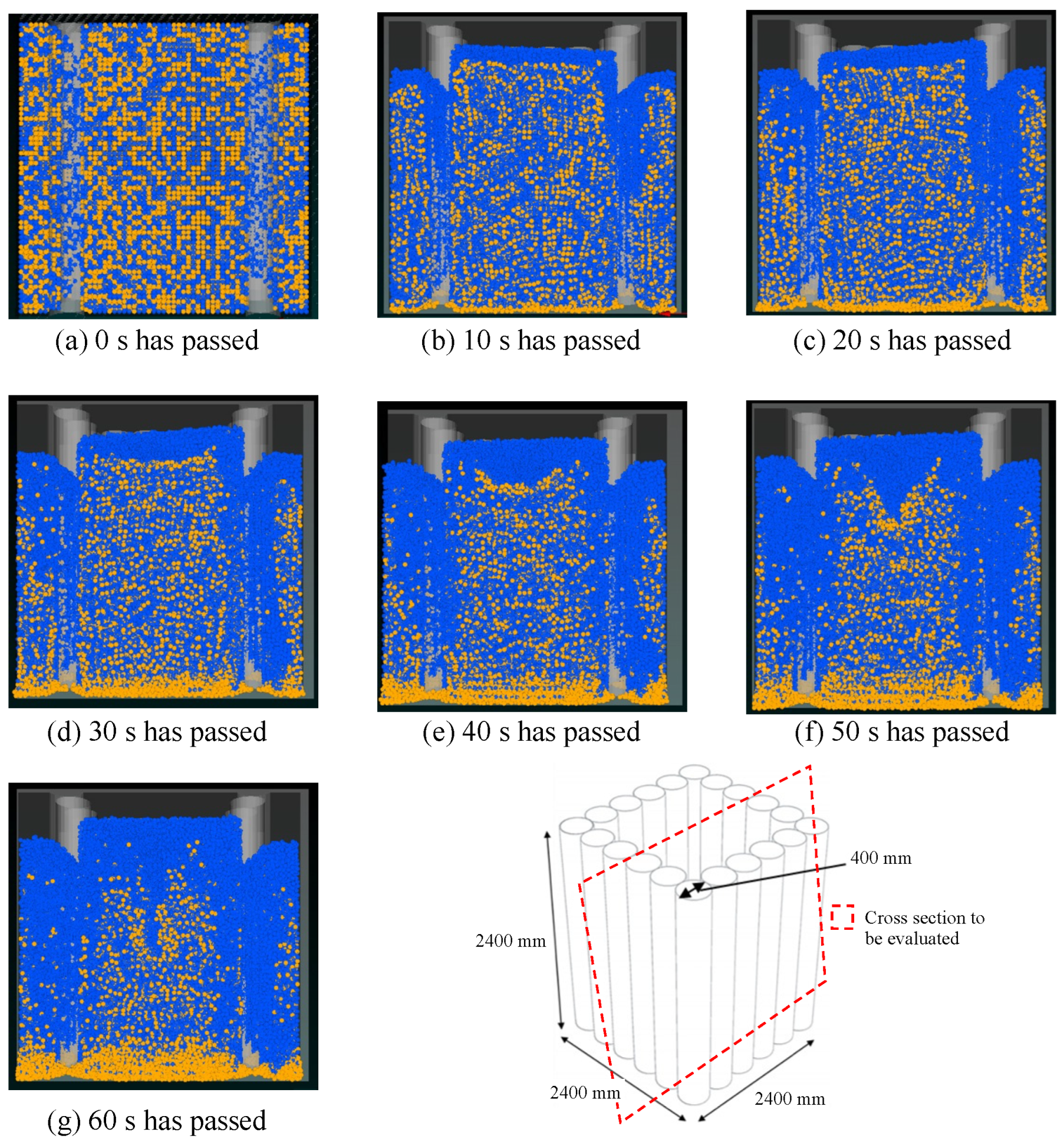
5. Results and Discussion

Figure 8, Figure 9 and Figure 10 show the simulation results for Cases 1, 2, and 3, respectively. These figures show the occurrence of liquefaction every 10 s from 0 s to 59.99 s. As the ground in Case 3 is surrounded by piles, Figure 10 shows the simulation results in a cross-sectional view. In all case studies, it is confirmed that the sand particles are deposited at the bottom of the analysis model over time and that the water particles are floating. In other words, this simulation was able to roughly recreate the liquefaction of the ground when an external acceleration, simulating seismic waves, was applied.
The mechanism of the liquefaction phenomenon is that when a sandy soil that is saturated with water experiences heavy shaking, the skeletal structure of the sand particles that make up the ground collapses, and the sand particles begin to filter down into the void spaces. As a result, excessive pore water pressure is generated and accumulates inside the ground. Furthermore, when the excess pore water pressure becomes equal to the effective loading pressure of the ground before it experiences heavy shaking, the effective stress loading between the soil particles becomes zero and, as a result of the above events, the liquefaction phenomenon occurs. The simulation results presented in Figure 8, Figure 9 and Figure 10 also show the same phenomenon as the above-mentioned liquefaction generation mechanism. In addition, when comparing the central part and the four corners of the analysis model in all cases, it is confirmed that the amount of sedimentation from the water particles in the four corners is smaller than that in the central part. This is because a rearrangement of the water particles and the sand particles occurs due to the external force, and the sand particles begin to settle and are deposited at the bottom of the model. While the sand particles settle and precipitate, the water particles rise to the top of the model. As a result, the sand particles are sedimented in the four corners at the bottom of the model and then flow out to the center of the model, resulting in a rearrangement of the particles.
When comparing Case 1 and Case 2 with different void ratios, it can be seen that the water particles in Case 1 are floating in the upper part of the model. It can be considered that this is the mechanism of the liquefaction phenomenon, that the loosely deposited sandy ground and the higher groundwater level are more likely to cause liquefaction. Comparing Case 1 and Case 3, with respect to the presence or absence of liquefaction countermeasures, the sand particles are stopped in the model at the inner part of the piles in Case 3. From this, it is thought that the liquefaction measures, wherein the ground is surrounded by piles, have been effective. The physical principle of the liquefaction countermeasure by piles is to keep the shear deformation caused by seismic motion small, block the propagation of pore water pressure from the surrounding soil, and prevent the outflow of pore water and sand into the supporting layers [40,41]. This simulation was able to reproduce the same phenomenon as in the physical principle of the liquefaction countermeasure that uses piles.
In this study, the MPSM-DEM coupled CAES was performed by the MPSM for pore water in the ground and the DEM for sand particles in the ground, and in a simulation of saturated sandy ground affected by seismic waves. The characteristics of this model were examined for elucidation of the liquefaction phenomenon. As a result of this simulation, the influence of the gap ratio on the liquefaction phenomenon and the influence of the presence or absence of liquefaction countermeasures were shown; it was confirmed that the purpose of the model construction was realized, at least qualitatively. Therefore, it was shown that the MPSM-DEM coupled CAES used in this study may be a method that can visualize various phenomena under the ground surface.

6. Conclusions

Based on the behavior of water particles and sand particles inside a model of the ground, in which the external acceleration simulating seismic waves affecting the ground was evaluated using an MPSM-DEM coupled CAES, an attempt was made to visualize the liquefaction phenomenon.
The results and findings obtained in this study are shown below.
(1)
Through the use of the MPSM-DEM coupled CAES, the liquefaction phenomenon was successfully visualized by applying an external acceleration that simulated seismic waves in the ground, modeled three-dimensionally.
(2)
The effect of the soil conditions, such as the void ratio, on the behavior of the particles in the soil during an earthquake was clarified. It was shown that, by employing the MPSM-DEM coupled CAES, it is possible to evaluate the behavior of the particles below the surface during an earthquake and to examine whether liquefaction is likely to occur.
(3)
The liquefaction phenomenon of a ground model with piles, simulating liquefaction countermeasures, was visualized. This visualization of the liquefaction phenomenon can be expected to contribute to the design and accountability of efficient and economical liquefaction countermeasures.
(4)
A MPSM-DEM coupled CAES model was constructed, in which the MPSM was used for the pore water below the surface and the DEM was used for the sand particles in the ground. In order to examine the validity of the constructed model, the authors conducted a numerical simulation with a model for the liquefaction phenomenon in a saturated sandy soil on which seismic waves acted, demonstrating the effectiveness of this model. From this, it was shown that an MPSM-DEM coupled CAES may be a method that can visualize various phenomena below the surface.
By utilizing the CAES for issues related to ground improvement, it is possible to visualize the earth below a construction site, which cannot otherwise be seen, and to solve complicated problems associated with construction. In addition, since the design and evaluation can be performed while comparing and examining various ground condition patterns, it is considered that the design quality can be improved at an early stage and a more effective construction method can be designed.
The subject of this study was to verify the validity of the simulation results and the model. It may be said that comparative verification is required to carry out laboratory experiments under the same conditions as the simulation conditions. In addition, the sand particles were set to have a single particle size of 20 mm in this study. However, because actual sandy soil contains particles of various sizes, it is unlikely that the reproducibility will be high. In addition, although the ground for which the liquefaction countermeasure work was simulated contained six piles placed on each of the four sides, there are other construction methods available, such as the arranging of double piles as part of actual liquefaction countermeasures construction. In order to visually evaluate the necessity of liquefaction countermeasures construction, the simulation and analysis of more case studies representing actual liquefaction countermeasures construction are required. Therefore, three issues remain to be solved: verification of the validity of the results, improvement of the reproducibility of actual sandy soil, and an evaluation/examination using a ground model that simulates more liquefaction countermeasures.

Author Contributions

Conceptualization, S.I., S.N.; methodology, K.N.; software, K.N.; validation, S.I., T.T., S.N.; formal analysis, K.N.; investigation, T.T.; resources, S.I.; data curation, K.N.; writing—original draft preparation, S.I.; writing—review and editing, S.N.; visualization, K.N.; supervision, S.I., S.N.; project administration, S.I.; funding acquisition, T.T. All authors have read and agreed to the published version of the manuscript.

Funding

This research received no external funding.

Institutional Review Board Statement

Not applicable.

Informed Consent Statement

Not applicable.

Data Availability Statement

Data sharing is applicable to this article.

Conflicts of Interest

The authors declare no conflict of interest.

References

  1. Kuribyashi, E.; Tatsuoka, F. Brief review of liquefaction during earthquakes in Japan. Soils Found. 1975, 15, 81–92. [Google Scholar] [CrossRef] [Green Version]
  2. Onoue, A.; Yasuda, S.; Toyota, H.; Inotsume, T.; Kiku, H.; Yamada, S.; Hosaka, Y.; Tsukamoto, Y.; Towhata, I.; Wakai, A.; et al. Review of Topographic and Soil Conditions for Liquefaction-Related Damage Induced by the 2007 Off Mid-Niigata Earthquake. Soils Found. 2011, 51, 533–548. [Google Scholar] [CrossRef] [Green Version]
  3. Yasuda, S.; Harada, K.; Ishikawa, K.; Kanemaru, Y. Characteristics of liquefaction in Tokyo Bay area by the 2011 Great East Japan Earthquake. Soils Found. 2012, 52, 793–810. [Google Scholar] [CrossRef] [Green Version]
  4. Cetin, K.O.; der Kiureghian, A.; Seed, R.B. Probabilistic models for the initiation of seismic soil liquefaction. Struct. Saf. 2002, 24, 67–82. [Google Scholar] [CrossRef]
  5. Chen, Z.; Li, H.; Goh, A.T.C.; Wu, C.; Zhang, W. Soil Liquefaction Assessment Using Soft Computing Approaches Based on Capacity Energy Concept. Geosciences 2020, 10, 330. [Google Scholar] [CrossRef]
  6. Huang, Y.; Yu, M. Review of soil liquefaction characteristics during major earthquakes of the twenty-first century. Nat. Hazards 2013, 65, 2375–2384. [Google Scholar] [CrossRef]
  7. Javdanian, H. Evaluation of soil liquefaction potential using energy approach: Experimental and statistical investigation. Bull. Eng. Geol. Environ. 2019, 78, 1697–1708. [Google Scholar] [CrossRef]
  8. Kirkwood, P.; Dashti, S. Considerations for the Mitigation of Earthquake-Induced Soil Liquefaction in Urban Environments. J. Geotech. Geoenviron. Eng. 2018, 144, 10. [Google Scholar] [CrossRef]
  9. Moss, R.E.; Seed, R.B.; Kayen, R.E.; Stewart, J.P.; der Kiureghian, A.; Cetin, K.O. CPT-Based Probabilistic and Deterministic Assessment of In Situ Seismic Soil Liquefaction Potential. J. Geotech. Geoenviron. Eng. 2006, 132, 1032–1051. [Google Scholar] [CrossRef] [Green Version]
  10. Uyanık, O. Soil liquefaction analysis based on soil and earthquake parameters. J. Appl. Geophys. 2020, 176, 104004. [Google Scholar] [CrossRef]
  11. Zhang, W.; Goh, A.T.; Zhang, Y.; Chen, Y.; Xiao, Y. Assessment of soil liquefaction based on capacity energy concept and multivariate adaptive regression splines. Eng. Geol. 2015, 188, 29–37. [Google Scholar] [CrossRef]
  12. Inazumi, S.; Jotisankasa, A.; Nakao, K.; Chaiprakaikeow, S. Performance of mechanical agitation type of ground-improvement by CAE system using 3-D DEM. Results Eng. 2020, 6, 100108. [Google Scholar] [CrossRef]
  13. Inazumi, S.; Kuwahara, S.; Jotisankasa, A.; Chaiprakaikeow, S. MPS-CAE simulation on dynamic interaction between steel casing and existing pile when pulling out existing piles. Int. J. GEOMATE Geotech. Constr. Mater. Environ. 2020, 18, 68–73. [Google Scholar] [CrossRef]
  14. Kazama, M.; Kawai, T.; Mori, T.; Kim, J.; Yamazaki, T. Subjects of the Liquefaction Research Seen to the Liquefaction Damage of the Great East Japan Earthquake Disaster. J. Jpn. Assoc. Earthq. Eng. 2018, 18, 26–39. [Google Scholar] [CrossRef] [Green Version]
  15. Rapti, I.; Lopez-Caballero, F.; Modaressi-Farahmand-Razavi, A.; Foucault, A.; Voldoire, F. Liquefaction analysis and damage evaluation of embankment-type structures. Acta Geotech. 2018, 13, 1041–1059. [Google Scholar] [CrossRef] [Green Version]
  16. Finn, W. State-of-the-art of geotechnical earthquake engineering practice. Soil Dyn. Earthq. Eng. 2000, 20, 1–15. [Google Scholar] [CrossRef] [Green Version]
  17. Wu, W.; Lin, J.; Wang, X. A basic hypoplastic constitutive model for sand. Acta Geotech. 2017, 12, 1373–1382. [Google Scholar] [CrossRef] [Green Version]
  18. Tasiopoulou, P.; Gerolymos, N. Constitutive modeling of sand: Formulation of a new plasticity approach. Soil Dyn. Earthq. Eng. 2016, 82, 205–221. [Google Scholar] [CrossRef]
  19. Yasuda, S.; Yoshida, N.; Adachi, K.; Kiku, H.; Ishikawa, K. Simplified evaluation method of liquefaction-induced residual displacement. J. Jpn. Assoc. Earthq. Eng. 2017, 17, 1–20. [Google Scholar] [CrossRef] [Green Version]
  20. Yasuda, S.; Yoshida, N.; Adachi, K.; Kiku, H.; Gose, S.; Masuda, T. A simplified practical method for evaluating liquefaction-induced flow. J. Geotech. Eng. 1999, 638, 71–89. [Google Scholar] [CrossRef] [Green Version]
  21. Uzuoka, R.; Yashima, A.; Kawakami, T.; Konrad, J.-M. Fluid dynamics based prediction of liquefaction induced lateral spreading. Comput. Geotech. 1998, 22, 243–282. [Google Scholar] [CrossRef]
  22. Chang, K.H. Product Design Modeling Using CAD/CAE: The Computer Aided Engineering Design Series; Elsevier: Amsterdam, The Netherlands, 2014. [Google Scholar]
  23. Pan, Z.; Wang, X.; Teng, R.; Cao, X. Computer-aided design-while-engineering technology in top-down modeling of mechanical product. Comput. Ind. 2016, 75, 151–161. [Google Scholar] [CrossRef]
  24. Inazumi, S.; Tanaka, S.; Komaki, T.; Kuwahara, S. Effect of insertion of casing by rotation on existing piles in removal of existing pile. Geotech. Res. 2021, 8, 25–37. [Google Scholar] [CrossRef]
  25. Adeli, H.; Kumar, S. Distributed Computer-Aided Engineering for Analysis, Design, and Visualization; CRC Press: Boca Raton, FL, USA, 2020. [Google Scholar]
  26. Sanyal, J.; Goldin, G.M.; Zhu, H.; Kee, R.J. A particle-based model for predicting the effective conductivities of composite electrodes. J. Power Sources 2010, 195, 6671–6679. [Google Scholar] [CrossRef]
  27. Nohara, S.; Suenaga, H.; Nakamura, K. Large deformation simulations of geomaterials using moving particle semi-implicit method. J. Rock Mech. Geotech. Eng. 2018, 10, 1122–1132. [Google Scholar] [CrossRef]
  28. Inazumi, S.; Kaneko, M.; Shigematsu, Y.; Shishido, K.-I. Fluidity evaluation of fluidisation treated soils based on the moving particle semi-implicit method. Int. J. Geotech. Eng. 2018, 12, 325–336. [Google Scholar] [CrossRef]
  29. Zhu, C.; Chen, A.; Huang, Y. Coupled Moving Particle Simulation–Finite-Element Method Analysis of Fluid–Structure Interaction in Geodisasters. Int. J. Géoméch. 2021, 21, 04021081. [Google Scholar] [CrossRef]
  30. Inazumi, S.; Kaneko, M.; Tomoda, Y.; Shigematsu, Y.; Shishido, K. Evaluation of flow-ability on fluidization treated soils based on flow analysis by MPS method. Int. J. GEOMAT Geotech. Constr. Mater. Environ. 2017, 12, 53–58. [Google Scholar] [CrossRef]
  31. Cundall, P.A.; Hart, R.D. Numerical Modeling of Discontinua. In Analysis and Design Methods; Elsevier: Amsterdam, The Netherlands, 1993; Chapter 9; pp. 231–243. [Google Scholar] [CrossRef]
  32. Cundall, P.A. A discontinuous future for numerical modelling in geomechanics? Geotech. Eng. 2001, 149, 41–47. [Google Scholar] [CrossRef]
  33. Miyamura, T.; Ohsaki, M.; Kajiwara, K. Seismic response analysis of super-highrise steel building frame modeled using solid elements: Analysis under simulated ground motions of Great Nankai Trough earthquakes that continuue more than two minutes. J. Struct. Constr. Eng. 2019, 84, 39–49. [Google Scholar] [CrossRef]
  34. Ucgul, M.; Saunders, C.; Fielke, J.M. Comparison of the discrete element and finite element methods to model the interaction of soil and tool cutting edge. Biosyst. Eng. 2018, 169, 199–208. [Google Scholar] [CrossRef]
  35. Wang, S.; Qu, T.; Fang, Y.; Fu, J.; Yang, J. Stress Responses Associated with Earth Pressure Balance Shield Tunneling in Dry Granular Ground Using the Discrete-Element Method. Int. J. Géoméch. 2019, 19, 7. [Google Scholar] [CrossRef]
  36. Hang, C.; Gao, X.; Yuan, M.; Huang, Y.; Zhu, R. Discrete element simulations and experiments of soil disturbance as affected by the tine spacing of subsoiler. Biosyst. Eng. 2018, 168, 73–82. [Google Scholar] [CrossRef]
  37. Tan, X.; Li, W.; Zhao, M.; Tam, V.W.Y. Numerical Discrete-Element Method Investigation on Failure Process of Recycled Aggregate Concrete. J. Mater. Civ. Eng. 2019, 31, 1. [Google Scholar] [CrossRef]
  38. Zhu, J.; Ma, T.; Lin, Z.; Xu, J.; Qiu, X. Evaluation of internal pore structure of porous asphalt concrete based on laboratory testing and discrete-element modeling. Constr. Build. Mater. 2021, 273, 121754. [Google Scholar] [CrossRef]
  39. Antoniou, A.; Daudeville, L.; Marin, P.; Omar, A.; Potapov, S. Discrete element modelling of concrete structures under hard impact by ogive-nose steel projectiles. Eur. Phys. J. Spéc. Top. 2018, 227, 143–154. [Google Scholar] [CrossRef]
  40. Harada, E.; Gotoh, H.; Ikari, H.; Khayyer, A. Numerical simulation for sediment transport using MPS-DEM coupling model. Adv. Water Resour. 2019, 129, 354–364. [Google Scholar] [CrossRef]
  41. Harada, E.; Ikari, H.; Khayyer, A.; Gotoh, H. Numerical simulation for swash morphodynamics by DEM–MPS coupling model. Coast. Eng. J. 2018, 61, 2–14. [Google Scholar] [CrossRef]
Figure 1. Calculation algorithm of the moving particle semi-implicit method.
Sustainability 14 07517 g001
Figure 2. Modeled contact forces between particles in DEM.
Sustainability 14 07517 g002
Figure 3. Calculation algorithm of DEM.
Sustainability 14 07517 g003
Figure 8. Liquefaction occurrence from 0 to 60 s in Case 1, when external acceleration is applied (void ratio: 1.19).
Sustainability 14 07517 g008
Figure 9. Liquefaction occurrence from 0 to 60 s in Case 2, when external acceleration is applied (void ratio: 0.71).
Sustainability 14 07517 g009
Figure 10. Liquefaction occurrence from 0 to 60 s in Case 3, when external acceleration is applied (void ratio: 1.19).
Sustainability 14 07517 g010
Table 1. The MPSM parameters adopted for the pore water.
Density ρ (kg/m3) Coefficient of Kinematic Viscosity υ (m2/s)
Pore water9980.000001
Table 2. The DEM parameters adopted for the sand particles.
Sand Particles
Particle density ρ (kg/m3)2634
Normal spring constant k n (N/m)1.0 × 108
Tangent spring constant k t (N/m)2.5 × 107
Normal attenuation constant η n 0.7
Tangent attenuation constant η t 0.7
Frictional coefficient μ 0.5
Table 3. The simulation conditions for Cases 1 to 3.
Void RatioLiquefaction Countermeasure
Case 11.19Without countermeasure
Case 20.71Without countermeasure
Case 31.19With countermeasure
Publisher’s Note: MDPI stays neutral with regard to jurisdictional claims in published maps and institutional affiliations.

