Article

Developing a 3D Hydrodynamic and Water Quality Model for Floating Treatment Wetlands to Study the Flow Structure and Nutrient Removal Performance of Different Configurations

1
PowerChina Northwest Engineering Corporation Limited, Xi’an 710065, China
2
State Key Laboratory of Eco-Hydraulics in Northwest Arid Region of China, Xi’an University of Technology, Xi’an 710048, China
3
State Key Laboratory of Hydraulic Engineering Simulation and Safety, Tianjin University, Tianjin 300072, China
*
Author to whom correspondence should be addressed.
Sustainability 2022, 14(12), 7495; https://doi.org/10.3390/su14127495
Submission received: 9 May 2022 / Revised: 15 June 2022 / Accepted: 16 June 2022 / Published: 20 June 2022

Abstract

:
Floating treatment wetlands (FTWs) are widely used in surface water. The nutrient removal performance depends on both physical processes and chemical/biological transformations in FTWs. However, research describing the coupling processes of hydrodynamic and water quality in the system remains limited. Therefore, a coupled three-dimensional model of hydrodynamic and water quality for FTWs was developed based on the Environmental Fluid Dynamics Code (EFDC). Additional plant drag terms were added to the momentum equations to simulate the suspended canopy effect, and the chemical/biological processes occurring in FTWs were integrated into the original water quality equations simultaneously. The fully calibrated model was used to compare the hydrodynamic characteristics and nutrient removal performance of seven FTW configurations. The modeling results showed that the main stream would turn to the bottom and side of the plant root zone because of the block in FTWs. The differences in the hydrodynamic characteristics among the seven configurations led to a difference in water quality improvement effects. Segmenting a single FTW into a pair of parallel FTWs could achieve the maximum nitrogen and phosphorus mass removal. The results of the study are useful for designing an optimal FTW configuration in surface water.

1. Introduction

Floating treatment wetlands (FTWs) consist of emergent vegetation established upon a floating structure and have proved to be an effective and promising remediation technology for the removal of nutrients from surface water systems [1,2]. A large number of studies have demonstrated that FTWs could enhance the removal of suspended solids [3], nutrients [4], organic matter [5], metals [6] and algae [7]. The excellent nutrient removal performance benefits from the physical and chemical/biological processes occurring in the plant zone of the FTWs [8,9].
A physical experiment is a basic method to explore the hydrodynamic characteristics and nutrient removal processes that occur in FTWs. However, it is difficult to consider both processes as they are limited by space scale, time scale and numerous uncertain factors, such as temperature, wind and precipitation. On the one hand, some water quality models, which describe the physical and chemical/biological processes in FTWs, have been developed [10,11,12]. For example, Wang et al. [13] developed a FTWMOD model, which consisted of a plant growth module, a nitrogen dynamic module and a phosphorus dynamics module.
On the other hand, some researchers have tried to develop a hydrodynamic aquatic model, using Delft3D-FLOW, EFDC and Fluent, to study the effects of plants on hydrodynamic characteristics [9,14,15,16], without considering the chemical/biological processes caused by plants in FTWs. Therefore, a group of coupled models of hydrodynamics and water quality emerged. For example, Machado et al. [17] used numerical modeling with a reactive tracer to study the flow through the plant root zone, with the goal of determining which configuration of FTWs demonstrated higher nutrient removal performance. Sabokrouhiyeh et al. [18] developed a two-dimensional depth-averaged model to identify optimal vegetation distributions. However, the complex chemical/biological processes occurring in the plant zone of the FTWs were simplified as a degradation coefficient. An integrated model that considers both the flow and the complex chemical/biological processes is still unavailable thus far.
FTWs were always deployed in groups in surface water systems [19,20]. An unreasonable arrangement of FTWs might lead to dead-zones and associated short-circuiting in the FTW system [2,21,22], which could reduce the residential time and the rate of flow through the plant root zone, resulting in reduced nutrient removal performance. When two FTWs were arranged in series, the main stream turned from the upper water to the bottom water when flowing through the upstream FTW, resulting in a decrease in the inflow mass to the downstream FTW. Machado et al. [17] reported that the mass removal by the downstream FTW was 2.7% less than the upstream FTW. Previous studies indicated that a reasonable FTW arrangement could improve the nutrient removal performance. The goal of this study was to develop a 3D hydrodynamic and water quality model to study the flow structure and nutrient removal performance of different FTW configurations.

2. Materials and Methods

2.1. EFDC Description

The Environmental Fluid Dynamics Code (EFDC), developed by Hamrick (1992) [23], is capable of simulating one-, two- or three-dimensional hydrodynamic, sediment transport and water quality of rivers, lakes and reservoirs. Based on the assumption of vertical hydrostatic pressure and Boussinesq approximation, the following continuity equations and momentum equations are proposed [23].
The continuity equations:
( m ζ ) t + ( m x H u ) x + ( m x H v ) y + ( m w ) z = Q H
( m ζ ) t + ( m y H 0 1 u d z ) x + ( m x H 0 1 v d z ) y = 0 1 Q H d z
The momentum equations:
( m H u ) t + ( m y H u u ) x + ( m x H v u ) y + ( m w u ) z ( m f + v m y x u m x y ) H v = m y H ( g ζ + p ) x m y ( h x z H x ) p z + z ( m 1 H A v u v ) + Q u F u H
( m H v ) t + ( m y H u v ) x + ( m x H v v ) y + ( m w u ) z + ( m f + v m y x u m x y ) H u = m x H ( g ζ + p ) y m x ( h y z H y ) p z + z ( m 1 H A v u z ) + Q v F v H
p z = g H ρ ρ 0 ρ 0
where H = h + ζ is the total water depth, h is the equilibrium water depth and ζ is surface displacement from the equilibrium; u, v and w are water velocity in the x, y and z directions, respectively; mx and my are metric coefficients, m = mx · my; QH is water inflow/outflow from the external sources; p is the physical pressure in excess of the reference density hydrostatic pressure; Av is the vertical turbulent momentum mixing coefficient; Qu and Qv are the source and sink terms; Fu and Fv are extensions to the original equations to represent the plant drag force, respectively.

2.2. Development of a Hydrodynamic and Water Quality Model for FTWs

Based on the basic hydrodynamic module of EFDC, additional plant drag terms were added to simulate the effect of FTWs on flow structure. The plant drag force was modeled using Fu and Fv as Equations (6) and (7) [24]:
F u = 1 2 C D ρ a u u 2 + v 2 + w 2
F v = 1 2 C D ρ a v u 2 + v 2 + w 2
where CD is the drag coefficient, ρ is the density of the water column and a is the projected area of the canopy per unit volume.
Then, based on the basic water quality module of EFDC, the chemical/biological processes occurring in FTWs were integrated into the original water quality equations as source/sink terms. Here follows a condensed description of the water quality model for FTWs (FTWMOD). For detailed equations for the chemical/biological processes of plants, nitrogen and phosphorus, refer to the previous study [13]. The FTWMOD consists of three interconnected submodels: (1) a plant growth submodel; (2) a nitrogen dynamics submodel; and (3) a phosphorus dynamics submodel. The plant growth submodel incorporates two state variables, namely shoot biomass and root biomass. Organic nitrogen, ammonia nitrogen and nitrate nitrogen in the water column are modeled in the nitrogen dynamic submodel. Organic phosphorus and phosphate in the water column are modeled in the phosphorus dynamics submodel.

2.3. Expression of FTW in Model

In the model, the study area is generally divided into several grids, where the plant species in the FTWs, if they exist, can be defined. For each species, the corresponding planting density, root length, root diameter and drag coefficient can be set. Once the model is run, the plant species for each grid is first determined in the horizontal direction. Because FTWs can fluctuate with the water level, the grid that the FTWs occupy is dynamic and is determined according to the current water depth and the length of plant roots at each time step. Then, based on the plant properties and hydrodynamic characteristics, the plant drag force and the quality of nutrient removal from the water are calculated.

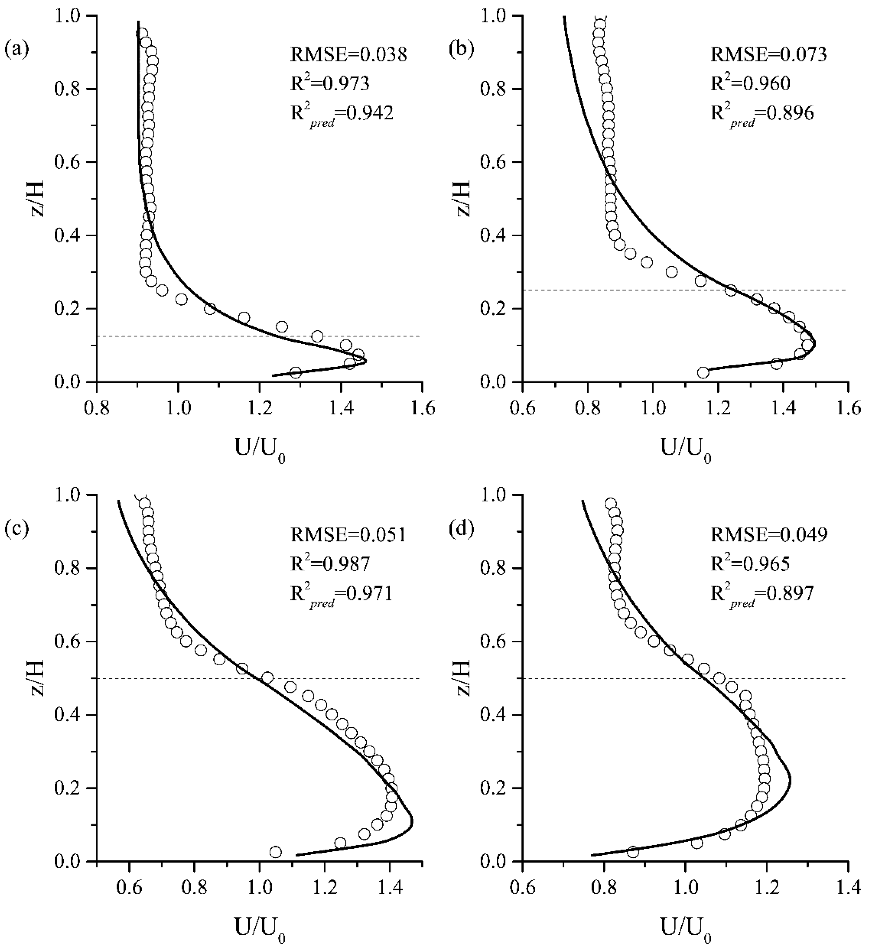
2.4. Calibration and Validation

The hydrodynamic model and water quality model for FTWs were calibrated separately due to the lack of relevant literature and experimental data for the simultaneous measurement of hydrodynamic and water quality data. The calibrated water quality model for FTWs in the previous study was used in the present study. Data for calibrating the hydrodynamic model were taken from laboratory experiments described by Plew [25] and were also used as calibrating data in other studies [9,24]. Results from four experiments (here termed B2, B5, B13 and B15) provide data for evaluating the hydrodynamic mode of FTWs. These experiments were conducted under steady flow conditions in an open channel flume with a length of 6.0 m and a width of 0.6 m. The plants used in the experiments, covering all the effective areas of the flume, were generalized as aluminum cylinders with a diameter of 9.54 mm. The basic conditions of the four experimental runs are listed in Table 1. The plant density in B2, B5 and B13 was the same, but the root length immersed in water was 175, 150 and 100 mm, respectively, and the flow rate was 7.1, 7.8 and 10.1 L/s, respectively. The root length immersed in water and the flow rate in B13 and B15 were the same, but the projected area per unit volume was 1.272 and 0.477 m2/m3, respectively, which meant the plant density was different. All the data described in this section were only used for model calibration and validation.
The three-dimensional hydrodynamic and water quality coupling model for B2, B5, B13 and B15 experimental runs was established. The size of the model mesh was 5.0 × 5.0 cm2 in the horizontal direction, and the water was evenly divided into 30 layers in the vertical direction, which suggested that the model had a total grid of 43,200. The roughness height was set to 0.001 m according to the previous study [24]. When the root length immersed in water was 175 mm (B2), the plant ranged from layer 5 to layer 30 (from bottom to top); when the root length immersed in water was 150 mm (B5), the plant ranged from layer 9 to layer 30; when the root length immersed in water was 100 mm (B13 and B15), the plant ranged from layer 16 to 30. After the model ran stably, the horizontal velocity along the vertical direction in the flume 4 m from the inlet was exported for comparison with the experimental data.
The root mean square error (RMSE), the coefficient of determination (R2) and the Predicted R-Squared (R2pred) were applied to evaluate the deviation between the experimental data and the simulation data:
RMSE = i = 1 N ( M i S i ) 2 N
R 2 = [ N i = 1 N M i S i ( i = 1 N M i ) ( i = 1 N S i ) N i = 1 N M i 2 ( i = 1 N M i ) 2 N i = 1 N S i 2 ( i = 1 N S i ) 2 ] 2
R p r e d 2 = 1 [ i = 1 N ( M i S i ) 2 i = 1 N ( S i M ¯ ) 2 ]
where Mi and Si are the experimental data and simulation data, respectively; M ¯ is the average value of the experimental data; and N is the number of data sets.

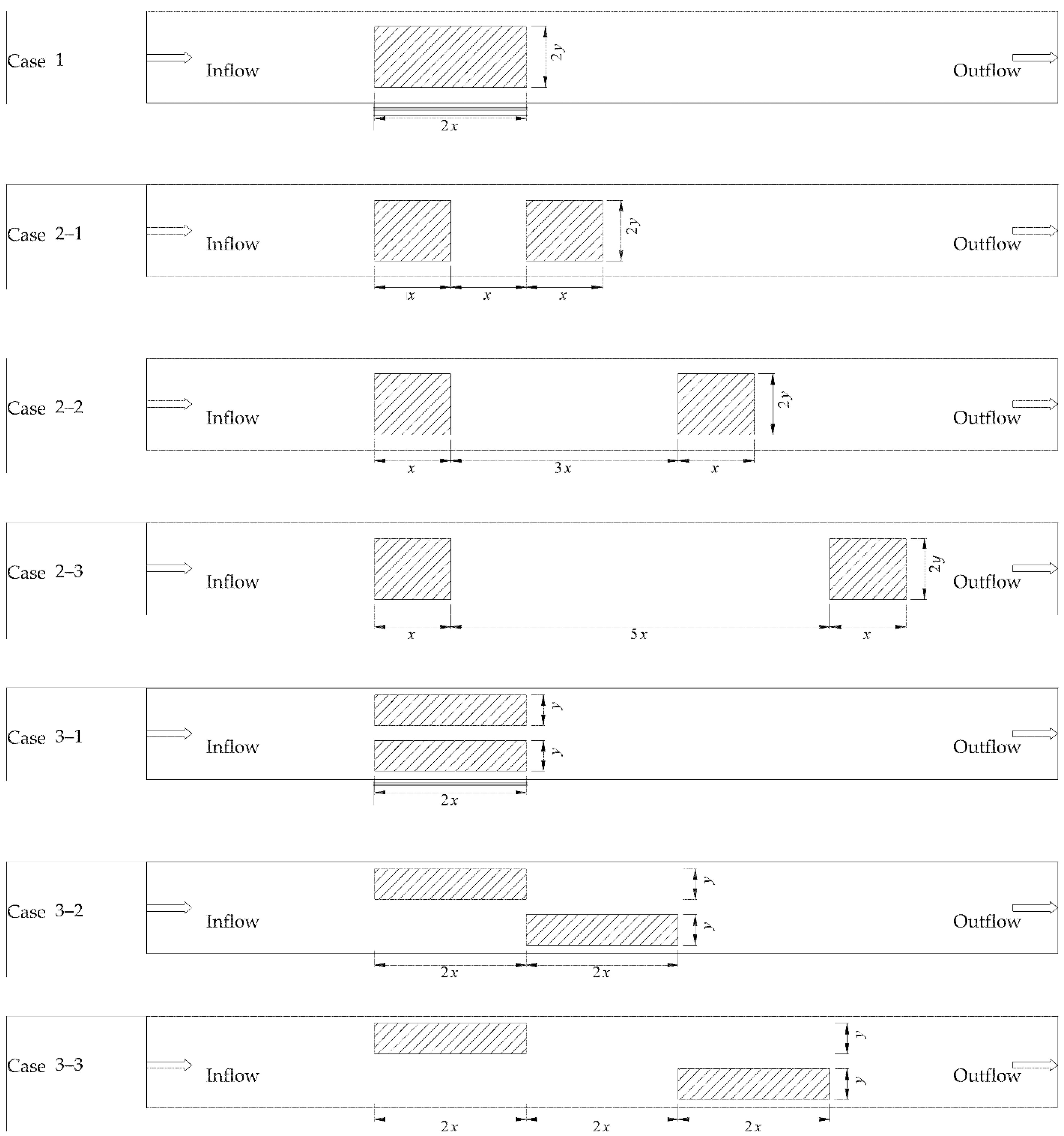
2.5. Model Application

To study the influence of the flow structure and the nutrient removal performance of different FTW configurations, the following seven typical cases were put forward in the open channel flume according to the layout form and spacing of the FTWs (Figure 1). A single large FTW was positioned in the channel flume in case 1. A single large FTW was evenly segmented into two smaller FTWs in series, and had distances of x, 3x and 5x in case 2–1, case 2–2 and case 2–3, respectively (x is the length of the two smaller FTWs). A single large FTW was evenly segmented into two smaller FTWs, which were interlaced at a distance of 0, 2x and 4x. For all cases, FTWs were arranged at a distance of 1.5 m from the inflow port to make sure that the water flow through the FTWs was steady. The root length immersed in water was 100 mm, and the area of the FTWs was 0.4 m2, occupying 11.1% of the water surface area. The inflow rate in all cases was 7.2 L/s with the same concentrations of NH4+–N (1.0 mg/L), NO3–N (1.0 mg/L), OrgN (1.0 mg/L), PO43−–P (0.1 mg/L) and OrgP (0.1 mg/L), while the water level at the outlet was maintained at 200 mm.
Because of the short contact time between nutrients and FTWs in the model application, the quality of the nutrients removed per unit time was used to evaluate the water quality improvement, which was also applied to practical engineering [26]. After the model ran stably, the quality of the nitrogen removed by FTWs within one day was calculated as:
N _ removal = 0 1 ( Plant _ N + Sed _ N + Denit _ N ) d t
Plant _ N = S ( L P L N M · B SH ( t , s ) + L P L N M · B RO ( t , s ) ) d s
Sed _ N = Ω K N S E D · OrgN ( t , x ) d x
Denit _ N = Ω D e n i t · NO 3 ( t , x ) d x
where N_removal is the quality of nitrogen removed by FTWs within one day; Plant_N is the net nitrogen content absorbed by plants; Sed_N is the accumulated nitrogen content in sediment; Denit_N is the nitrogen content removed via denitrification; LPLNM is the ratio of nitrogen to plant biomass; BSH and BRO are the shoot and root biomass of the plants, respectively; KNSED is the sedimentation rate of OrgN; Denit is the denitrification rate; OrgN and NO3 are the contents of organic nitrogen and nitrate nitrogen in the water column, s is the plane coordinate of the area covered with FTWs; x is the three-dimensional coordinate of the whole area.
The quality of the nitrogen removed by FTWs within one day was calculated as:
P _ removal = 0 1 ( Plant _ P + Sed _ P ) d t
Plant _ P = S ( L P L P M · B SH ( t , s ) + L P L P M · B RO ( t , s ) ) d s
Sed _ P = Ω ( K P S E D · OrgP ( t , x ) + K P C O · PO 4 ( t , x ) ) d x
where P_removal is the quality of the phosphorus removed by FTWs within one day; Plant_P is the net phosphorus content absorbed by plants; Sed_P is the accumulated phosphorus content in sediment; LPLPM is the ratio of phosphorus to plant biomass; KPSED is the sedimentation rate of OrgP; KPCO is the ratio of coprecipitation of PO43−–P.

3. Results and Discussion

3.1. Calibration and Validation Results

The simulation data about the horizontal velocity was exported and compared with the experimental data (Figure 2). The R2, R2pred and the RMSE were 0.973, 0.942 and 0.038 in B2; 0.960, 0.896 and 0.0378 in B5; 0.987, 0.971 and 0.051 in B13; and 0.965, 0.897 and 0.049 in B15, respectively. These results demonstrated the good performance of the hydrodynamic model for FTWs.

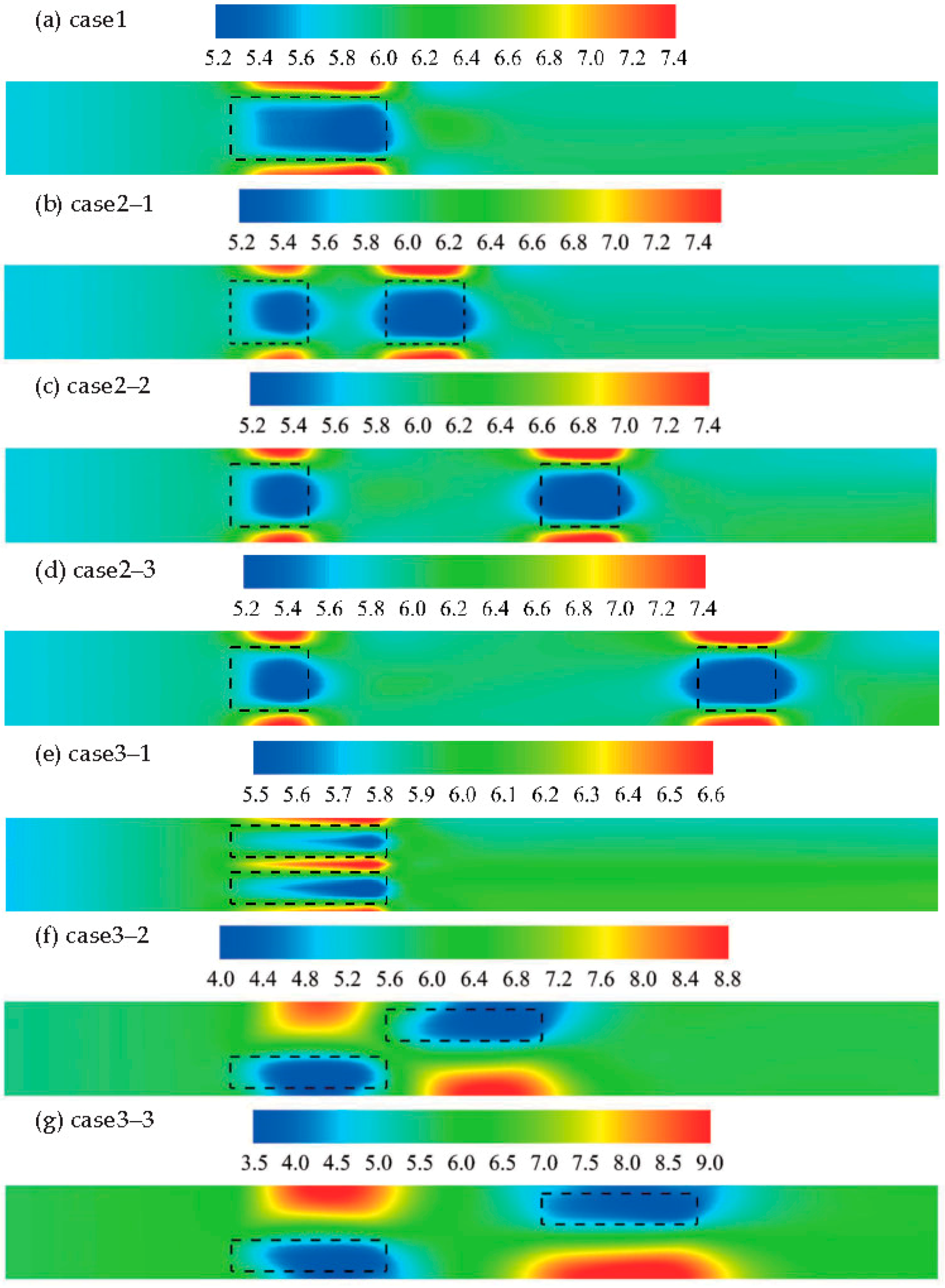
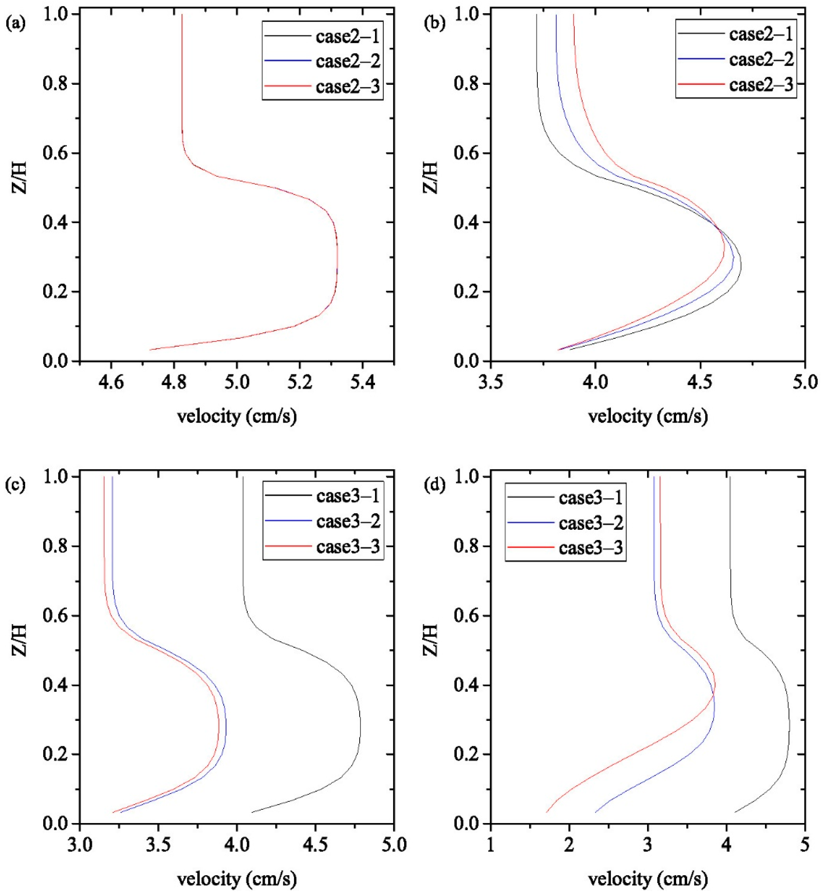
3.2. Flow Structure Comparison of Different FTW Configurations

The depth-averaged plane flow field and the horizontal velocity along the direction of the water depth are shown in Figure 3 and Figure 4, respectively. When a single large FTW was positioned in the channel flume (case 1), the main stream turned to the side and the bottom of the FTWs when entering the plant zone. The water flow velocity was minimized at the end of the FTW with an average of 5.09 cm/s, compared to 7.86 cm/s on the lateral sides of the FTW. As shown in Figure 4, because of the blocking of plant roots, the water flow velocity in the range of plant roots (4.97 cm/s) was lower than at the bottom (6.86 cm/s).
When a single large FTW was evenly segmented into two smaller FTWs in series (case 2–1, 2–2 and 2–3), the main stream turned to the side and the bottom of the FTWs when entering the plant zone of both FTWs. The three cases had similar flow characteristics around the first FTW, where the average velocity in and out of the range of plant roots was 4.84 cm/s and 5.22 cm/s, respectively. However, the average velocity in the plant zone of the second FTW increased with the distance of the two FTWs, which was 3.77 cm/s, 3.87 cm/s and 4.97 cm/s in case 2–1, 2–2 and 2–3, respectively.
When a single large FTW was evenly segmented into two smaller interlaced FTWs (case 3–1, 3–2 and 3–3), the average velocity in the range of plant roots of the upper FTW increased with the distance of the two staggered FTWs, which was 4.63 cm/s, 3.76 cm/s and 3.71 cm/s in case 3–1, 3–2 and 3–3, respectively. However, the average velocity in the range of plant roots of the lower FTW was reduced to 3.41 cm/s and 3.05 cm/s, respectively, when the distance of the two staggered FTWs was 2x (case 3–2) and 4x (case 3–3).

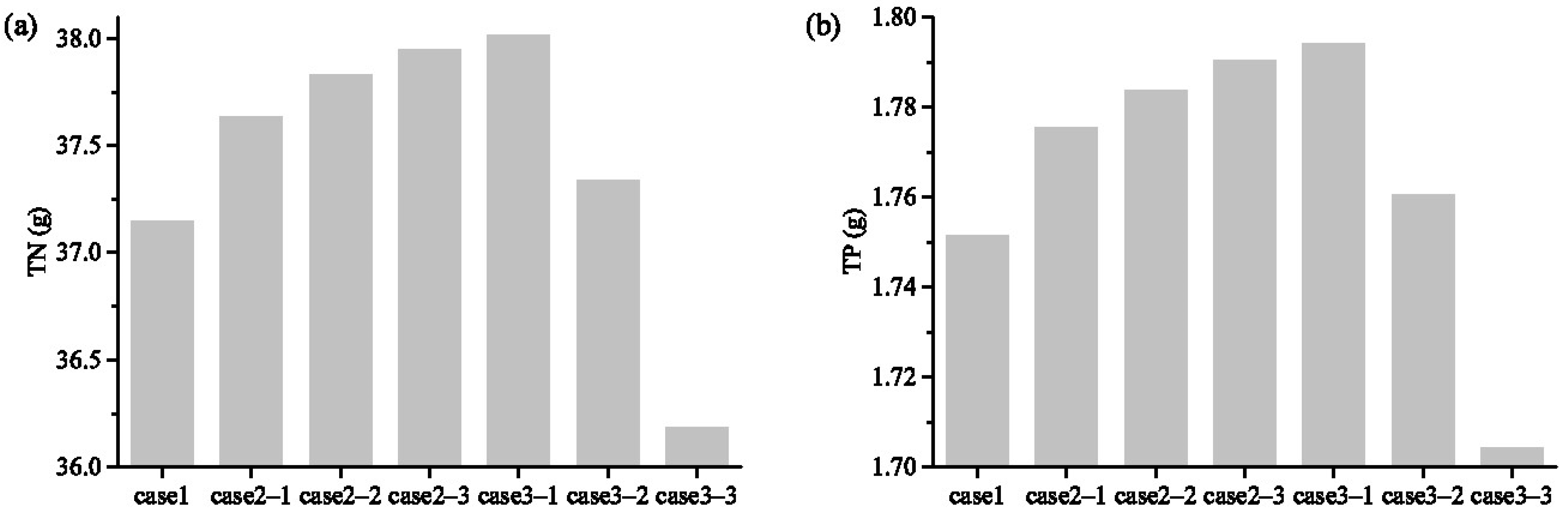
3.3. Nutrient Removal Performance Comparison of Different FTW Configurations

The quality of the nutrients removed per unit time in seven test cases is shown in Figure 5. When a single large FTW was positioned in the channel flume (case 1), the quality of TN and TP removed per unit time was 20.73 g and 0.97 g, respectively.
When a single large FTW was evenly segmented into two smaller FTWs in series (case 2–1, 2–2 and 2–3), the quality of the nutrients removed increased with the distance of the upper and lower FTWs. When the distance between the two FTWs was x, 3x and 5x, the removal quality of TN increased by 88.78 mg, 111.23 mg and 129.58 mg, respectively, compared with case 1; the removal quality of TP increased by 4.17 mg, 5.22 mg and 6.08 mg, respectively, compared with case 1.
When the two evenly segmented FTWs were arranged in parallel (case 3–1), the removal quality of TN and TP increased by 870.12 mg and 42.46 mg, respectively, which were the highest among all test cases. However, when the distance of the two staggered FTWs was increased, the nutrient removal performance declined substantially.
The center distance of two continuously arranged FTWs is an important factor for nutrient removal performance. A previous study proved that the fraction of flow entering the root zone of the FTW depended on the center distance [27]. When the center distance was 0.5 L, L and 11 L, where L was the length of the FTW along the flow direction, the percentages of the flow entering the root zone were 18 ± 8%, 52 ± 4% and 73 ± 2%, respectively [27]. When the percentage of flow entering the root zone increased, the nutrient removal performance should also be theoretically increased. This conclusion was consistent with Rao et al. [28], who found that when the center distance of two FTWs increased from 30 cm to 45 cm, the nutrient removal efficiency increased 20–40%. However, as the center distance increased, the surface area of the FTWs would inevitably be reduced in certain systems. Liu et al.’s study indicated that if the FTWs were continuously arranged with a center distance of 2–3 L in the whole area, then the system would have the highest nutrient removal performance [27].
Compared with FTWs deployed in series, FTWs deployed in a staggered formation had a greater impact on the flow structure, and the influence decreased along with the space between the two FTWs [29]. A higher turbulence intensity was beneficial to the absorption and diffusion of nutrients [8]. Computational fluid dynamics simulation results showed that when a single large FTW was evenly segmented into two smaller FTWs in parallel, the nutrient removal efficiency increased from 60% to 64% [17], which is consistent with our result.

4. Conclusions

This study developed a mathematical model by coupling both the hydrodynamic and chemical/biological processes in FWTs, which was then used to study the flow structure and nutrient removal performance of different FTW configurations. The main conclusions are as follows:
  • The calibration and validation results showed that the simulation results could be well matched with the experimental results. The hydrodynamic characteristics in FTWs could be described properly by the model.
  • When two FTWs were deployed in series, the percentage of the flow entering the root zone of the downstream FTW would increase with the center distance of two FTWs, resulting in higher TN and TP removal performance.
  • When two FTWs were deployed in parallel, the system had the highest TN and TP removal performance.
The model has potential for widespread application in FTW investigations and combines hydrodynamic and water quality to permit a comprehensive assessment of FTW arrangement in stormwater ponds and rivers. However, the model performance was only examined using a channel flume experiment; therefore, further examination of the model should be performed using a field-scale application. A field experiment will be planned in a stormwater pond or river to explore both the hydrodynamic characteristics and the nutrient removal performance, which could be helpful for improving the model.

Author Contributions

Conceptualization, Y.W. and X.G.; methodology, B.S.; software, Y.W. and Y.L.; validation, X.G., B.S. and Y.L.; formal analysis, B.S.; investigation, Y.W.; resources, X.G.; data curation, Y.L.; writing—original draft preparation, Y.W.; writing—review and editing, Y.L.; visualization, B.S. and Y.W.; supervision, B.S.; project administration, X.G.; funding acquisition, Y.W. All authors have read and agreed to the published version of the manuscript.

Funding

This research was funded by the Major Science and Technology Program for Water Pollution Control and Treatment (2018ZX07105-002), the Science Fund for Creative Research Group of the National Natural Science Foundation of China (51621092) and the Natural Science Foundation of Tianjin (15JCYBJC22600).

Institutional Review Board Statement

Not applicable.

Informed Consent Statement

Not applicable.

Data Availability Statement

Not applicable.

Conflicts of Interest

The authors declare no conflict of interest. The funders had no role in the design of the study; in the collection, analyses, or interpretation of data; in the writing of the manuscript, or in the decision to publish the results.

References

  1. Sharma, R.; Vymazal, J.; Malaviya, P. Application of floating treatment wetlands for stormwater runoff: A critical review of the recent developments with emphasis on heavy metals and nutrient removal. Sci. Total Environ. 2021, 777, 146044. [Google Scholar] [CrossRef] [PubMed]
  2. Walker, C.; Tondera, K.; Lucke, T. Stormwater treatment evaluation of a Constructed Floating Wetland after two years operation in an urban catchment. Sustainability 2017, 9, 1687. [Google Scholar] [CrossRef] [Green Version]
  3. Borne, K.E.; Fassman, E.A.; Tanner, C.C. Floating treatment wetland retrofit to improve stormwater pond performance for suspended solids, copper and zinc. Ecol. Eng. 2013, 54, 173–182. [Google Scholar] [CrossRef]
  4. McAndrew, B.; Ahn, C.; Spooner, J. Nitrogen and sediment capture of a floating treatment wetland on an urban stormwater retention pond-The case of the rain project. Sustainability 2016, 8, 972. [Google Scholar] [CrossRef] [Green Version]
  5. Hwang, J.I.; Hinz, F.O.; Albano, J.P.; Wilson, P.C. Enhanced dissipation of trace level organic contaminants by floating treatment wetlands established with two macrophyte species: A mesocosm study. Chemosphere 2021, 267. [Google Scholar] [CrossRef] [PubMed]
  6. Ning, D.; Huang, Y.; Pan, R.; Wang, F.; Wang, H. Effect of eco-remediation using planted floating bed system on nutrients and heavy metals in urban river water and sediment: A field study in China. Sci. Total Environ. 2014, 485–486, 596–603. [Google Scholar] [CrossRef]
  7. West, M.; Fenner, N.; Gough, R.; Freeman, C. Evaluation of algal bloom mitigation and nutrient removal in floating constructed wetlands with different macrophyte species. Ecol. Eng. 2017, 108, 581–588. [Google Scholar] [CrossRef] [Green Version]
  8. Nuruzzaman, M.; Anwar, A.H.M.F.; Sarukkalige, R.; Sarker, D.C. Review of hydraulics of Floating Treatment Islands retrofitted in waterbodies receiving stormwater. Sci. Total Environ. 2021, 801, 149526. [Google Scholar] [CrossRef]
  9. Li, S.; Katul, G.; Huai, W. Mean velocity and shear stress distribution in floating treatment wetlands: An analytical study. Water Resour. Res. 2019, 55, 6436–6449. [Google Scholar] [CrossRef]
  10. Cui, Z.; Huang, J.; Gao, J.; Han, J. Characterizing the impacts of macrophyte-dominated ponds on nitrogen sources and sinks by coupling multiscale models. Sci. Total Environ. 2022, 811, 152208. [Google Scholar] [CrossRef]
  11. McAndrew, B.; Ahn, C. Developing an ecosystem model of a floating wetland for water quality improvement on a stormwater pond. J. Environ. Manag. 2017, 202, 198–207. [Google Scholar] [CrossRef] [PubMed]
  12. Marimon, Z.A.; Xuan, Z.; Chang, N.B. System dynamics modeling with sensitivity analysis for floating treatment wetlands in a stormwater wet pond. Ecol Model 2013, 267, 66–79. [Google Scholar] [CrossRef]
  13. Wang, Y.; Sun, B.; Gao, X.; Li, N. Development and evaluation of a process-based model to assess nutrient removal in floating treatment wetlands. Sci. Total Environ. 2019, 694, 133633. [Google Scholar] [CrossRef] [PubMed]
  14. Zhao, F.; Huai, W.; Li, D. Numerical modeling of open channel flow with suspended canopy. Adv. Water Resour. 2017, 105, 132–143. [Google Scholar] [CrossRef]
  15. O’Donncha, F.; Hartnett, M.; Plew, D.R. Parameterizing suspended canopy effects in a three-dimensional hydrodynamic model. J. Hydraul. Res. 2015, 53, 714–727. [Google Scholar] [CrossRef]
  16. Sonnenwald, F.; Guymer, I.; Stovin, V. A CFD-based mixing model for vegetated flows. Water Resour. Res. 2019, 55, 2322–2347. [Google Scholar] [CrossRef] [Green Version]
  17. Machado Xavier, M.L.; Janzen, J.G.; Nepf, H. Numerical modeling study to compare the nutrient removal potential of different floating treatment island configurations in a stormwater pond. Ecol. Eng. 2018, 111, 78–84. [Google Scholar] [CrossRef] [Green Version]
  18. Sabokrouhiyeh, N.; Bottacin-Busolin, A.; Tregnaghi, M.; Nepf, H.; Marion, A. Variation in contaminant removal efficiency in free-water surface wetlands with heterogeneous vegetation density. Ecol. Eng. 2020, 143, 105662. [Google Scholar] [CrossRef]
  19. Song, J.; Li, Q.; Wang, X.C. Superposition effect of floating and fixed beds in series for enhancing nitrogen and phosphorus removal in a multistage pond system. Sci. Total Environ. 2019, 695, 133678. [Google Scholar] [CrossRef]
  20. Liu, J.; Wang, F.; Liu, W.; Tang, C.; Wu, C.; Wu, Y. Nutrient removal by up-scaling a hybrid floating treatment bed (HFTB) using plant and periphyton: From laboratory tank to polluted river. Bioresource Technol. 2016, 207, 142–149. [Google Scholar] [CrossRef]
  21. Borne, K.E.; Fassman-Beck, E.A.; Winston, R.J.; Hunt, W.F.; Tanner, C.C. Implementation and maintenance of floating treatment wetlands for urban stormwater management. J. Environ. Eng. 2015, 141, 04015030. [Google Scholar] [CrossRef]
  22. Lucke, T.; Walker, C.; Beecham, S. Experimental designs of field-based constructed floating wetland studies: A review. Sci. Total Environ. 2019, 660, 199–208. [Google Scholar] [CrossRef] [PubMed]
  23. Hamrick, J.M. A Three-Dimensional Environmental Fluid Dynamics Computer Code: Theoretical and Computational Aspects; Special Report in Applied Marine Science and Ocean Engineering; No. 317.; Virginia Institute of Marine Science, William & Mary: Williamsburg, VA, USA, 1992; pp. 9–11. [Google Scholar]
  24. James, S.C.; Donncha, F.O. Drag coefficient parameter estimation for aquaculture systems. Environ. Fluid Mech. 2019, 19, 989–1003. [Google Scholar] [CrossRef] [Green Version]
  25. Plew, D.R. Depth-averaged drag coefficient for modeling flow through suspended canopies. J. Hydraul. Eng. 2011, 137, 234–247. [Google Scholar] [CrossRef]
  26. Tripathi, B.D.; Srivastava, J.; Misra, K. Nitrogen and Phosphorus Removal-capacity of Four Chosen Aquatic Macrophytes in Tropical Freshwater Ponds. Environ. Conserv. 1991, 18, 143–147. [Google Scholar] [CrossRef]
  27. Liu, C.; Shan, Y.; Lei, J.; Nepf, H. Floating treatment islands in series along a channel: The impact of island spacing on the velocity field and estimated mass removal. Adv. Water Resour. 2019, 129, 222–231. [Google Scholar] [CrossRef]
  28. Rao, L.; Wang, P.; Lei, Y.; Wang, C. Coupling of the flow field and the purification efficiency in root system region of ecological floating bed under different hydrodynamic conditions. J. Hydrodyn. 2016, 28, 1049–1057. [Google Scholar] [CrossRef]
  29. Gao, Y.; Zhu, Q.; Huang, Y.; Yu, M.; Zhou, Z. Influence of different arrangements of ecological floating beds on flow structure. J. Hydraul. Eng. 2020, 51, 1423–1431. [Google Scholar]
Figure 1. Configuration of FTWs for 7 test cases in the model. The arrows mean flow direction and the boxes mean FTWs.
Sustainability 14 07495 g001
Figure 2. Comparison between simulated (solid line) and experimental (dots) for the normalized horizontal velocity in (a) B2, (b) B5, (c) B13 and (d) B15.
Sustainability 14 07495 g002
Figure 3. The depth-averaged plane flow field (cm/s). The dotted squares mean FTWs.
Sustainability 14 07495 g003
Figure 4. Velocity distribution in vertical line of the (a) upper FTW, (b) lower FTW in case 2–1, 2–2 and 2–3, and (c) upper FTW, (d) lower FTW in case 3–1, 3–2 and 3–3.
Sustainability 14 07495 g004
Figure 5. Quality of nutrients removed per unit time for 7 test cases, (a) TN, (b) TP.
Sustainability 14 07495 g005
Table 1. Basic condition of the B2, B5, B13 and B15 experimental runs.
RunH
(mm)
hg
(mm)
L
(mm)
B
(mm)
a
(m2/m3)
Q
(L/s)
B2200175150501.2727.1
B5200150150501.2727.8
B13200100150501.27210.1
B152001002001000.47710.3
Note. H is the water depth, hg is the root length immersed in water, L and B are the streamwise and cross-stream spacing between plants, a is the projected area per unit volume, Q is the flow rate.
Publisher’s Note: MDPI stays neutral with regard to jurisdictional claims in published maps and institutional affiliations.

