
Comparative Analysis of Accuracy, Simplicity and Generality of Temperature-Based Global Solar Radiation Models: Application to the Solar Map of Asturias


Abstract
:1. Introduction
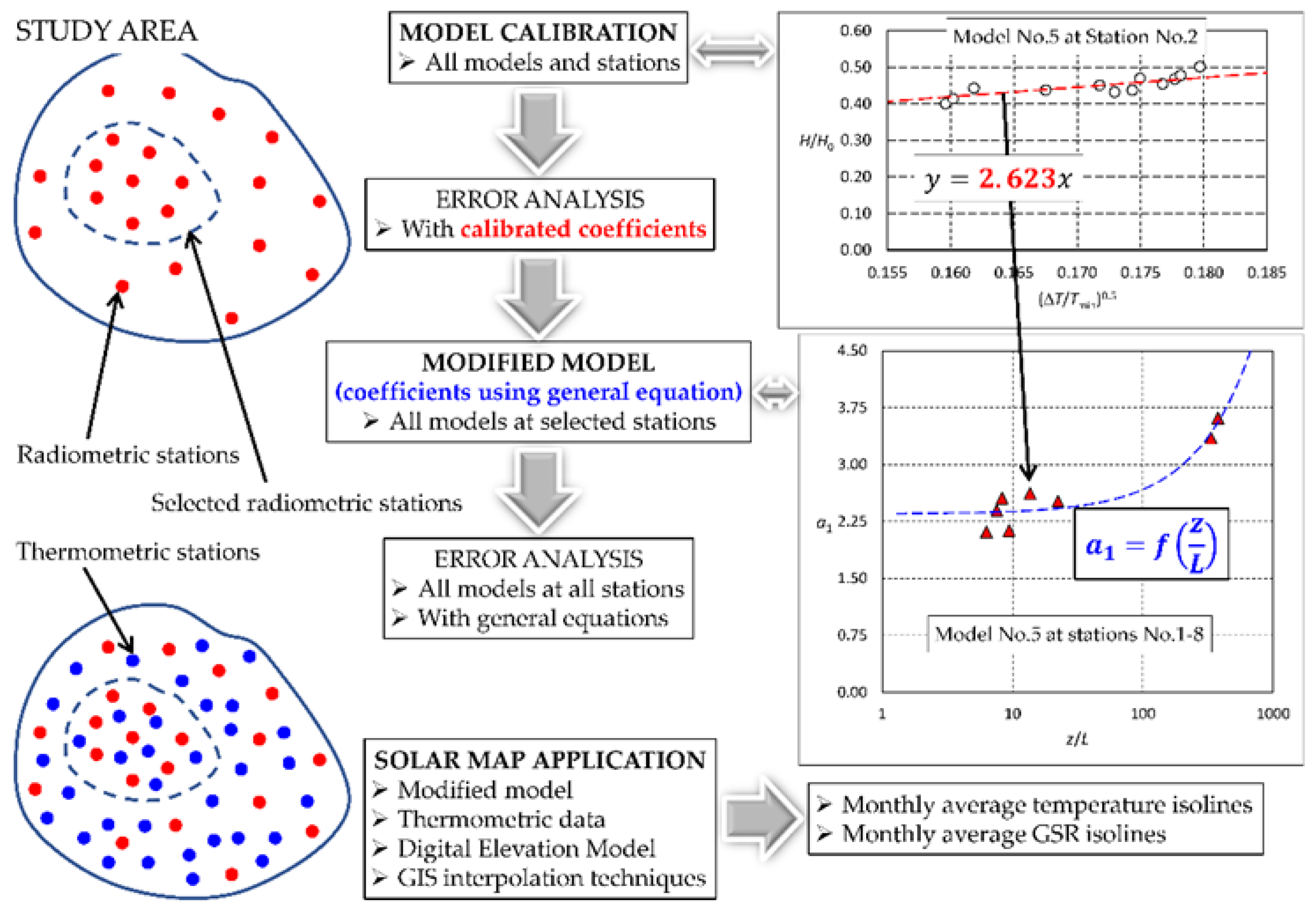
2. Materials and Methods
2.1. Selection of Temperature-Based GSR Models
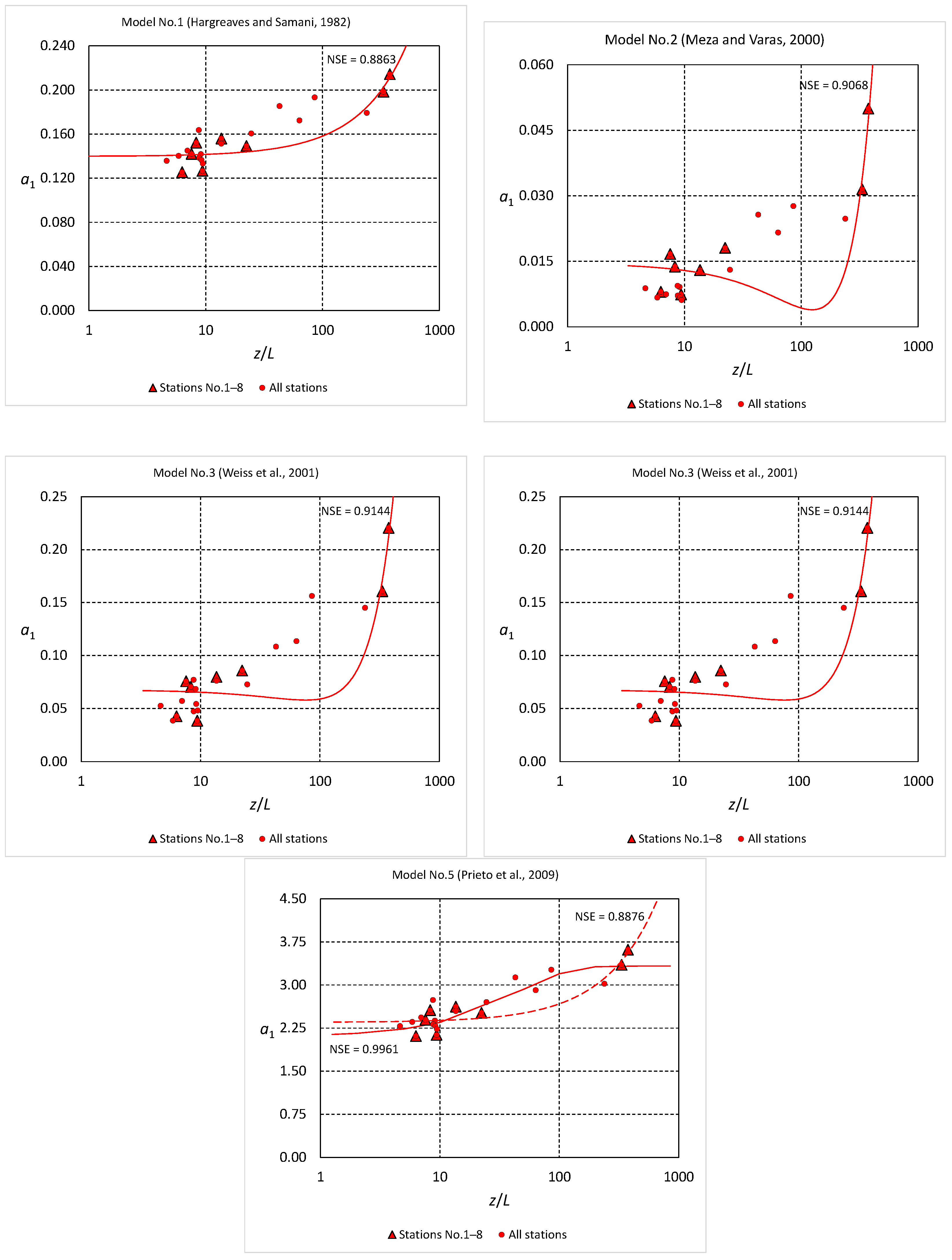
2.1.1. Model No.1: Hargreaves and Samani
2.1.2. Model No.2: Meza and Varas
2.1.3. Model No.3: Weiss et al.
2.1.4. Model No.4: Annandale et al.
2.1.5. Model No.5: Prieto et al.
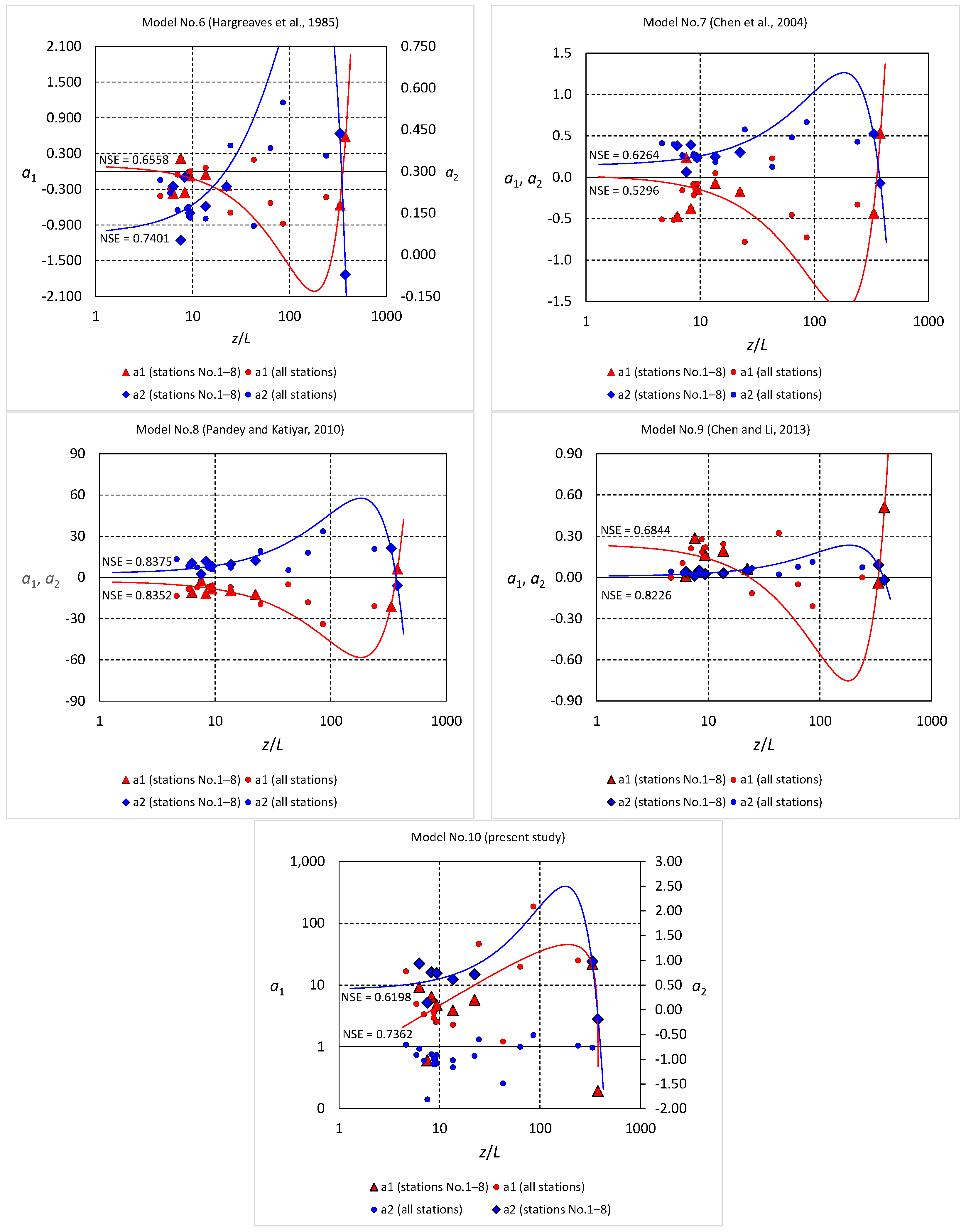
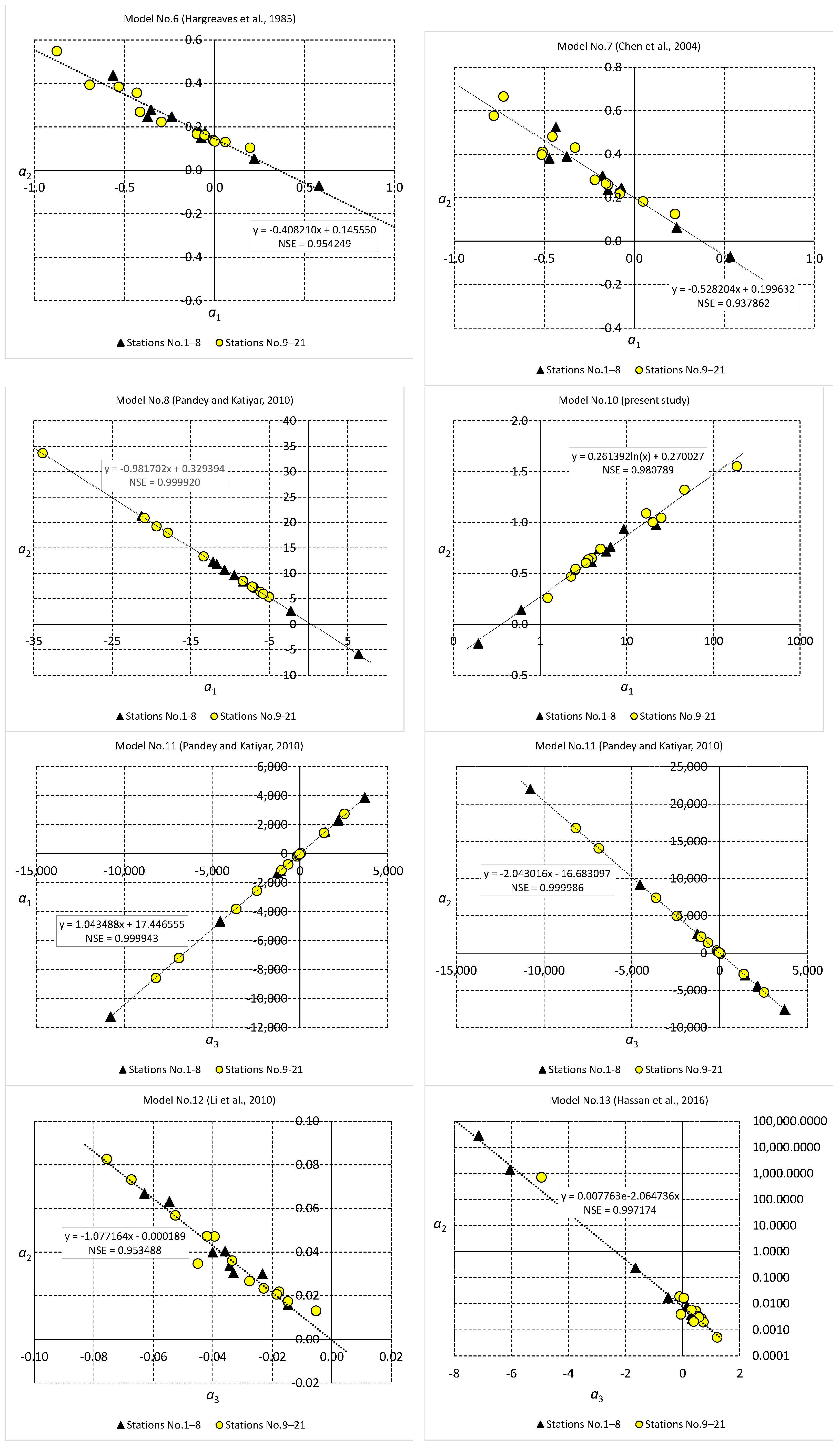
2.1.6. Model No.6: Hargreaves et al.
2.1.7. Model No.7: Chen et al.
2.1.8. Model No.8: Pandey and Katiyar
2.1.9. Model No.9: Chen and Li
2.1.10. Model No.10: Present Study
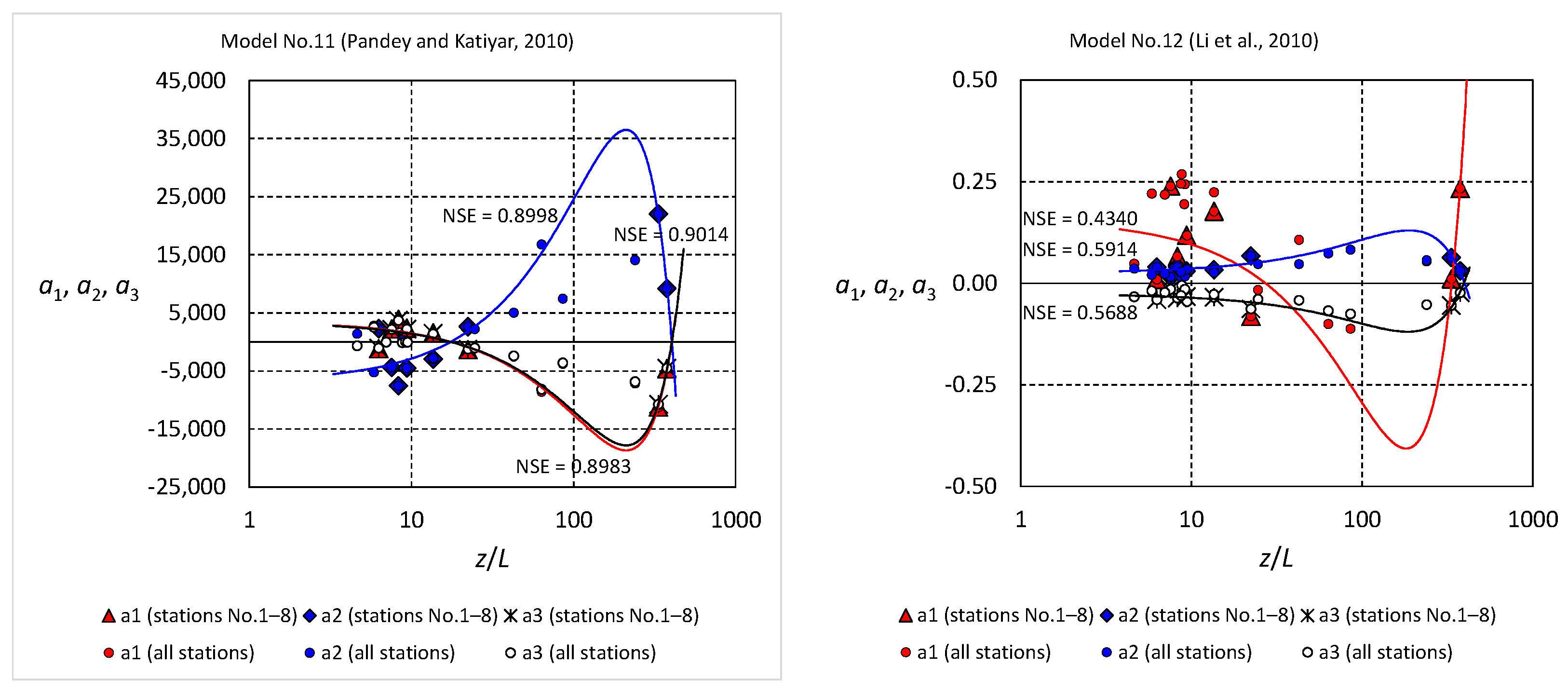
2.1.11. Model No.11: Pandey and Katiyar
2.1.12. Model No.12: Li et al.
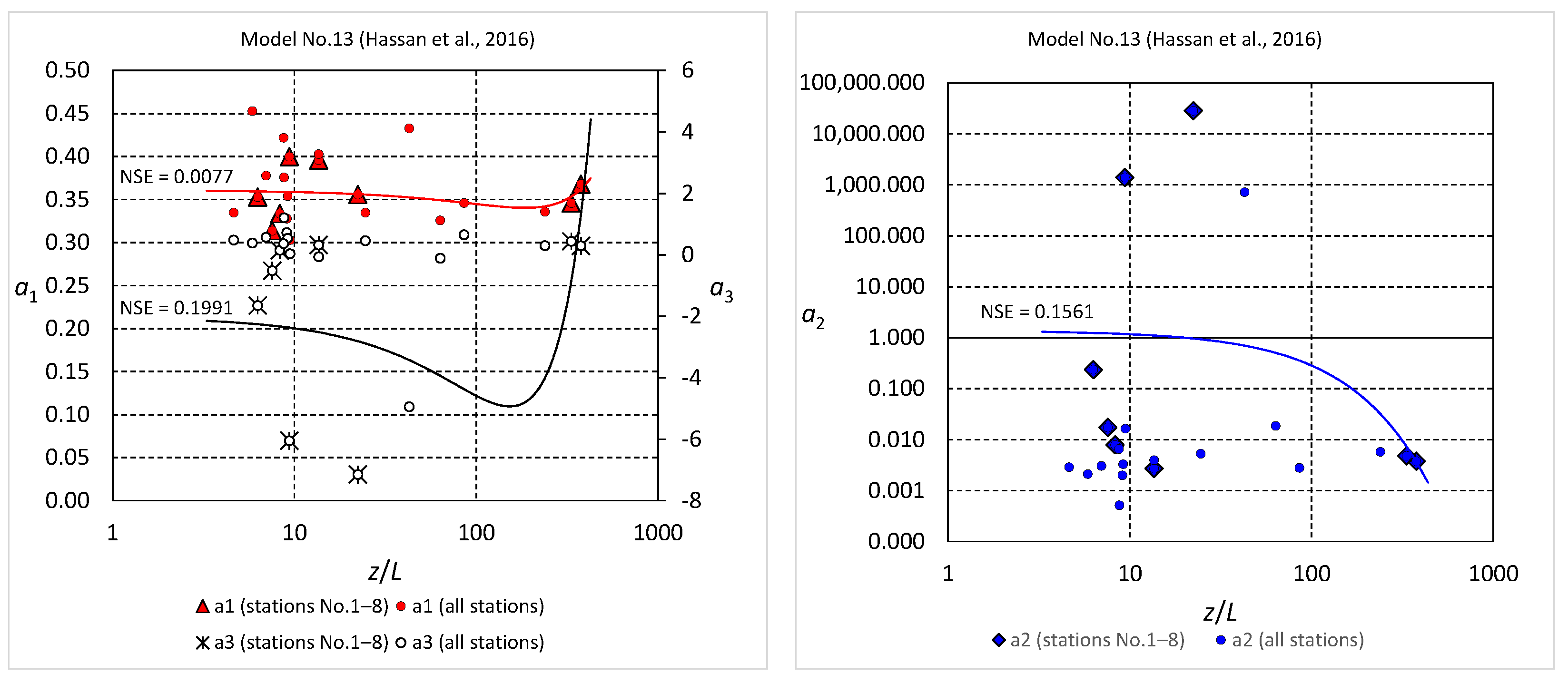
2.1.13. Model No.13: Hassan et al.
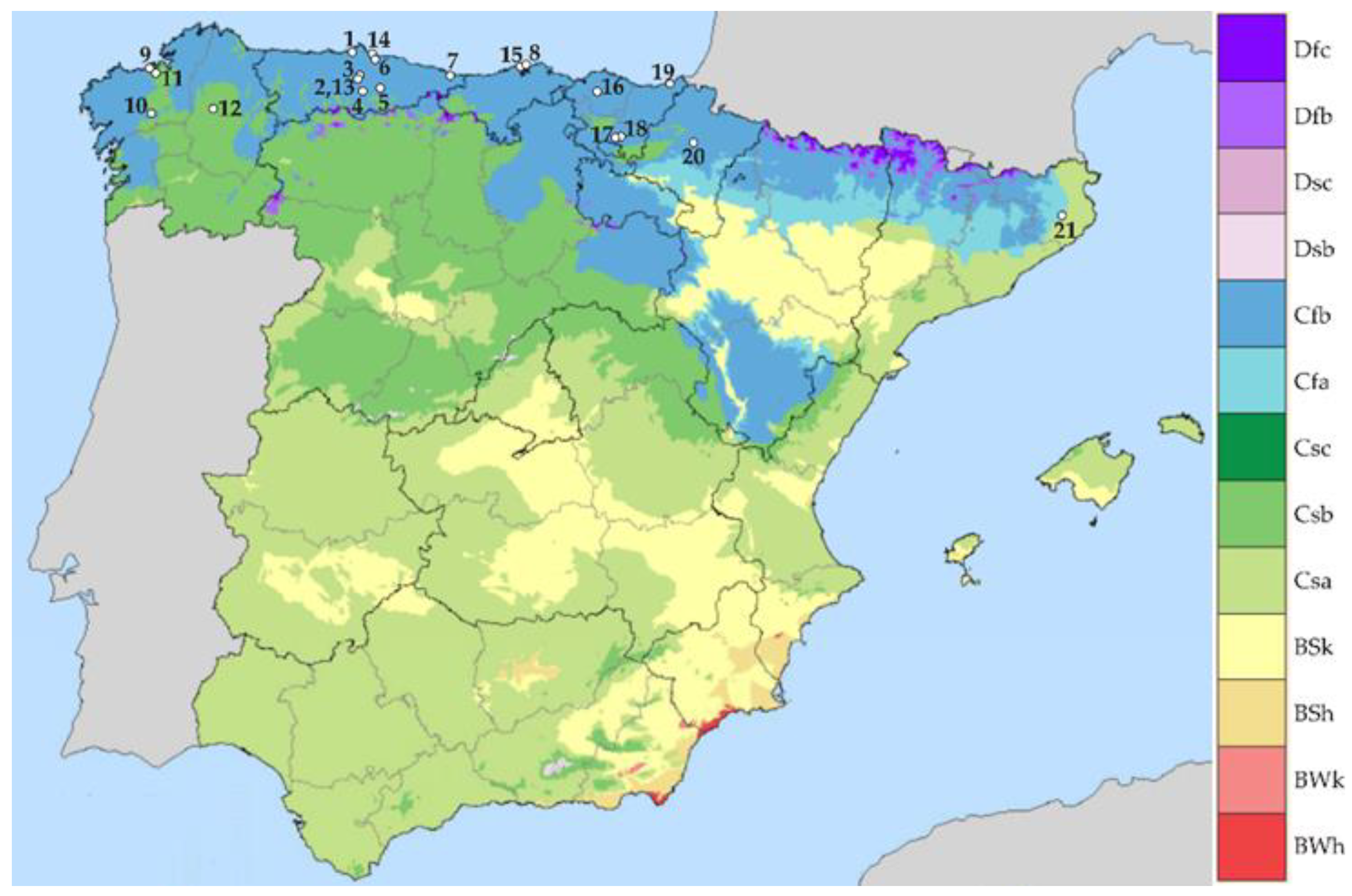
2.2. Meteorological Stations
2.3. Experimental Data
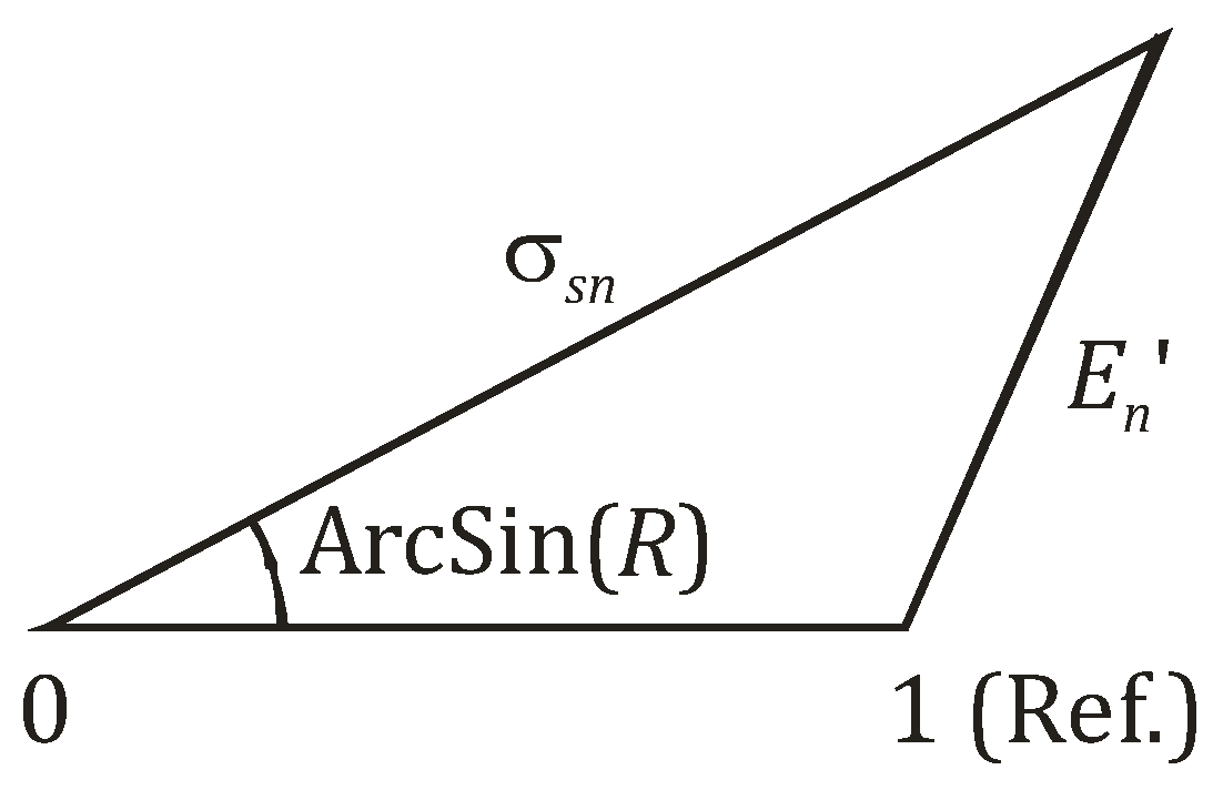
2.4. Statistical Indicators
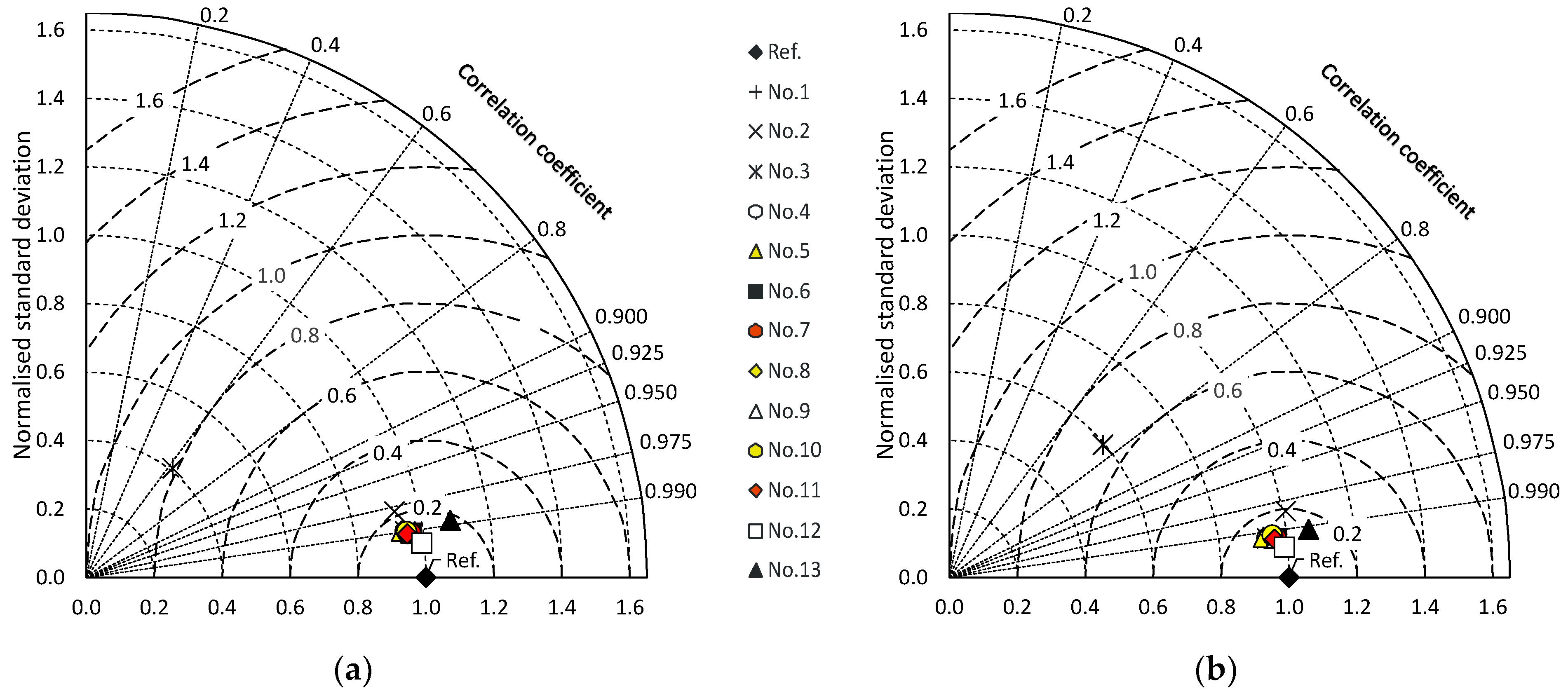
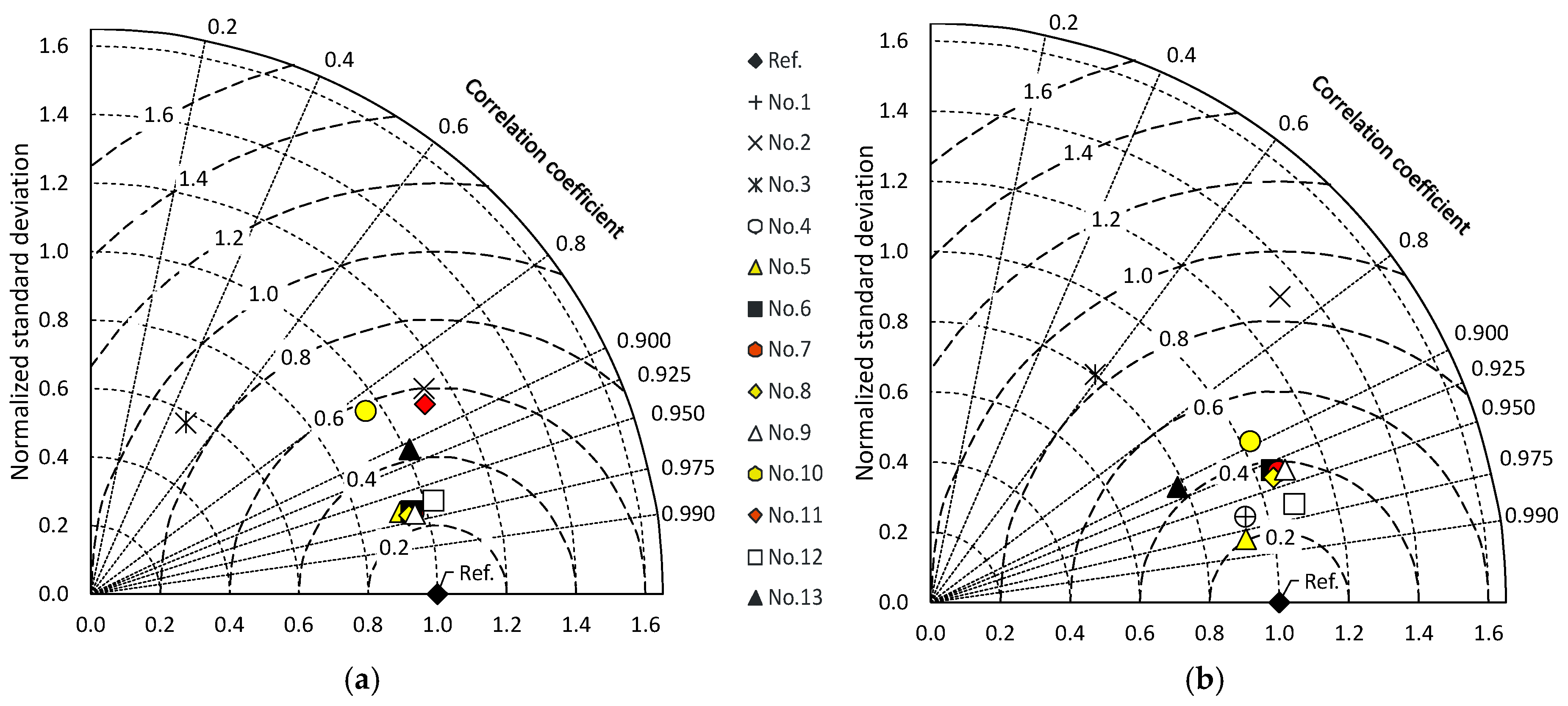
3. Results and Discussion
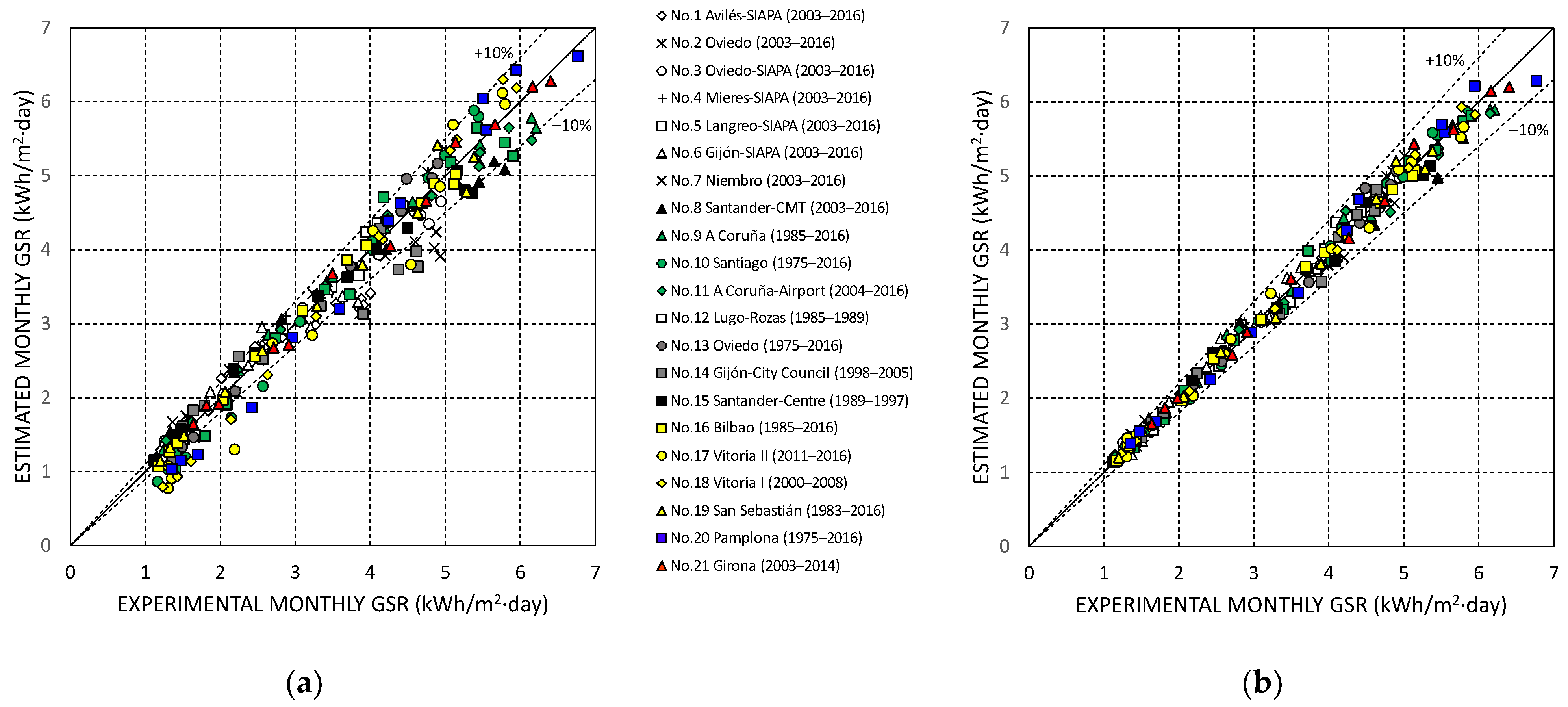
3.1. Model Performance with Site-Calibrated Coefficients
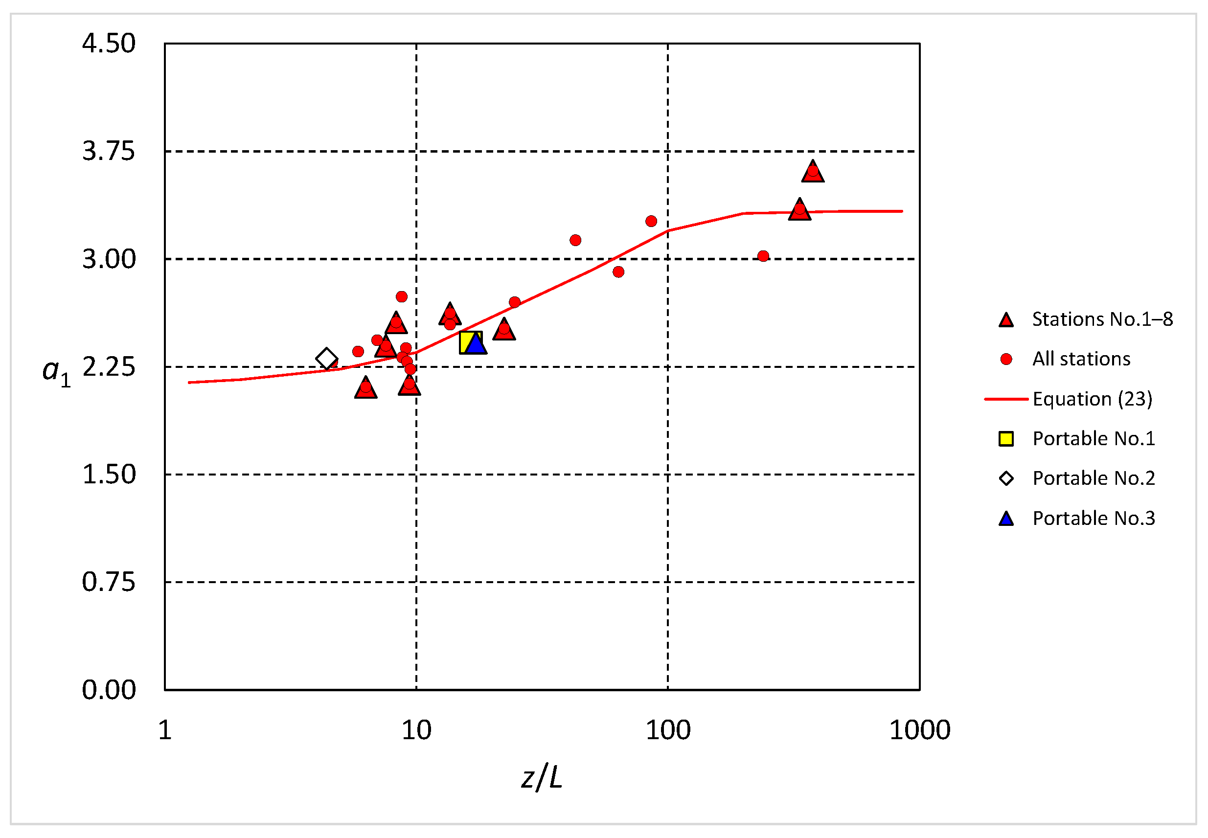
3.2. Model Performance with Coefficients Obtained from General Equations
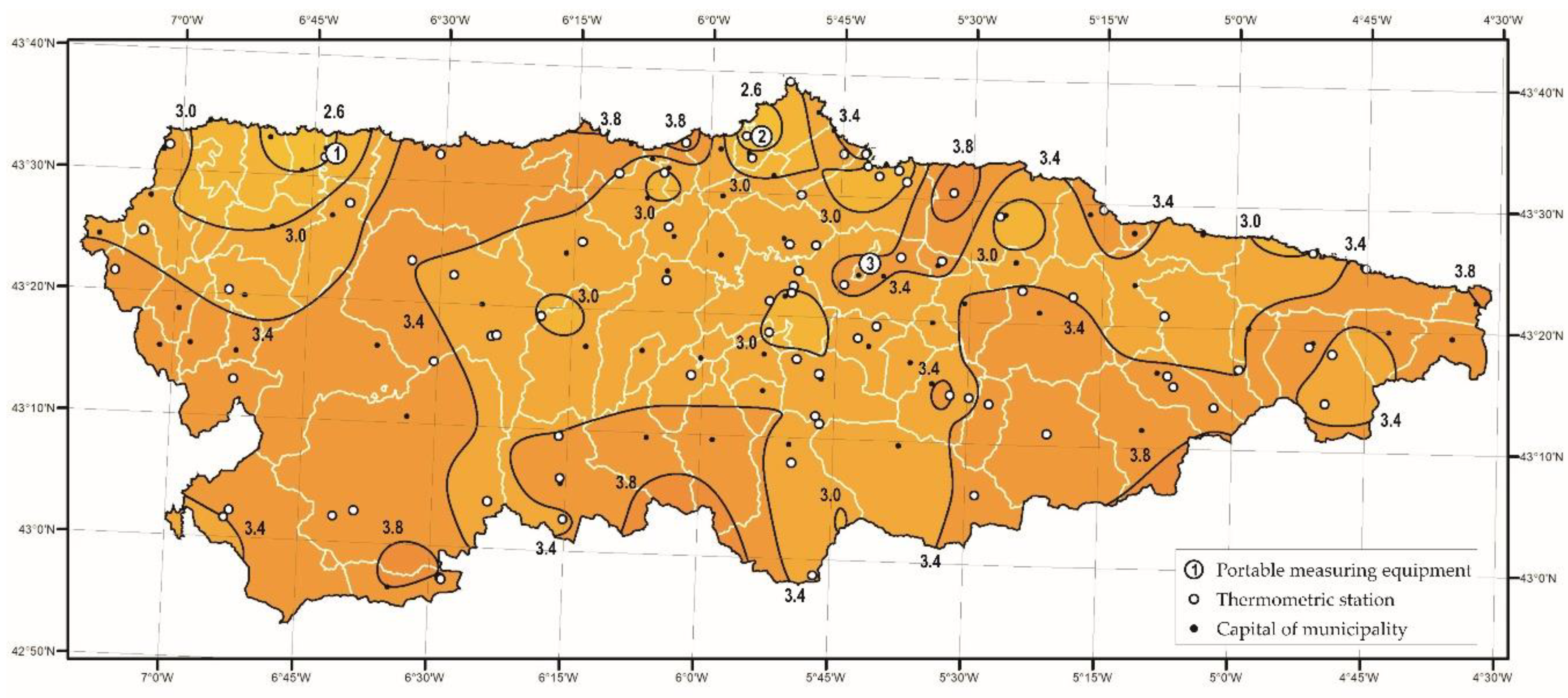
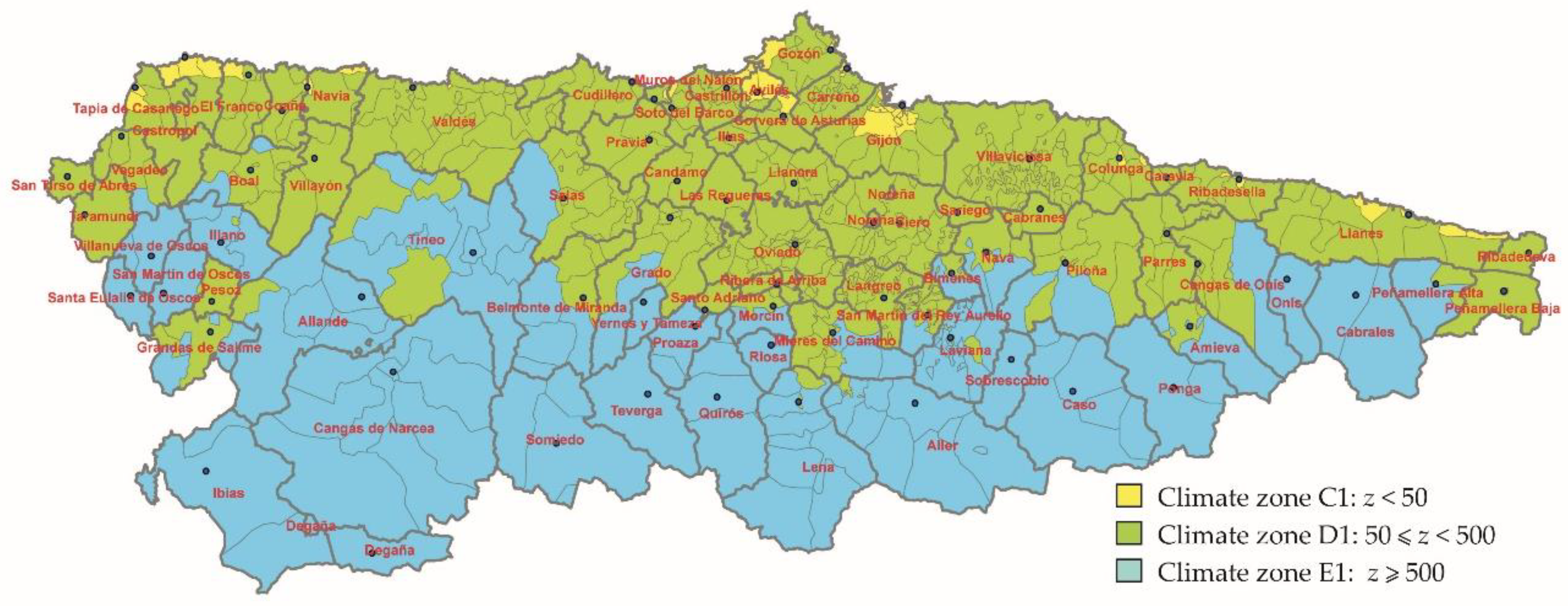
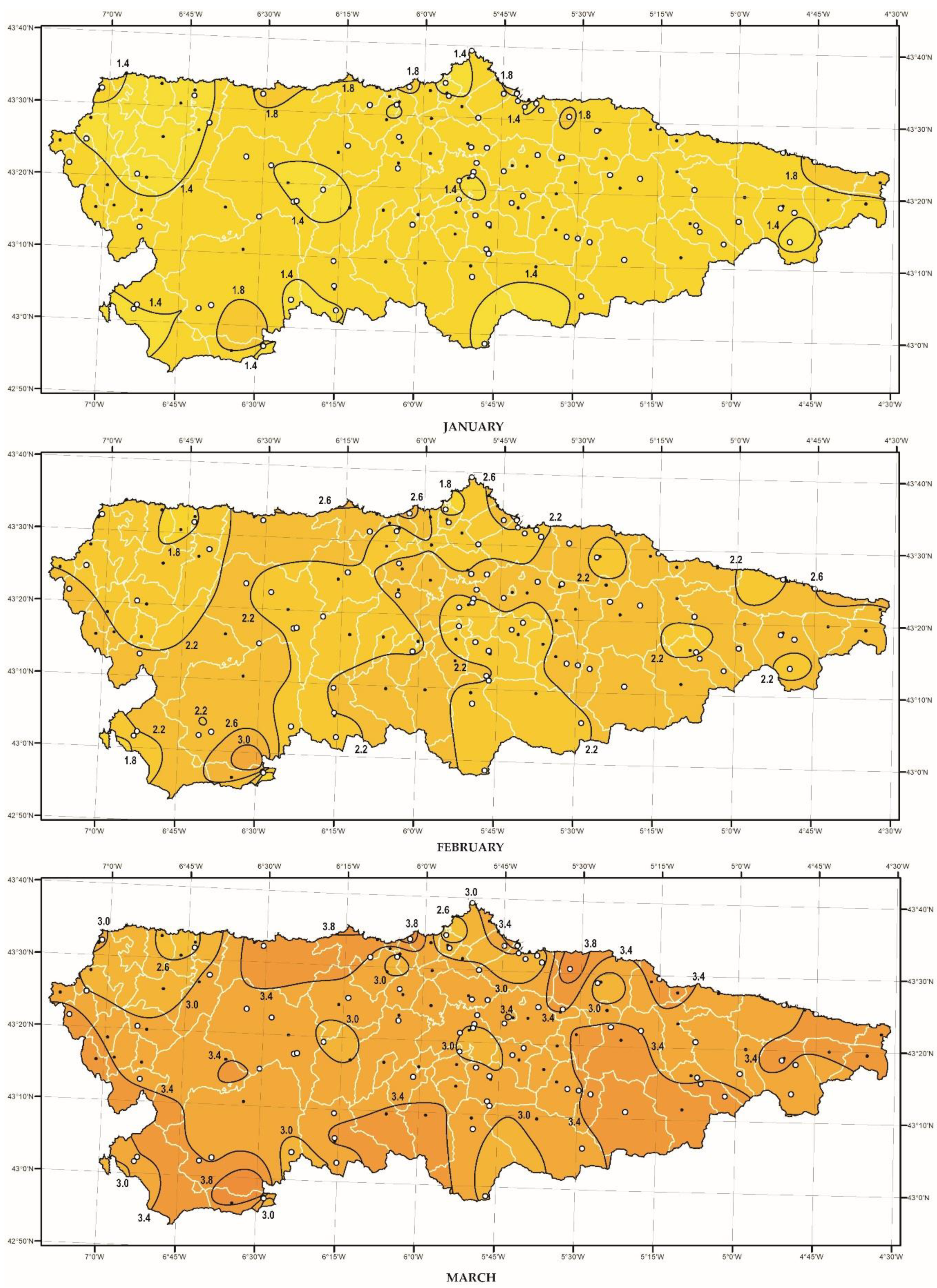
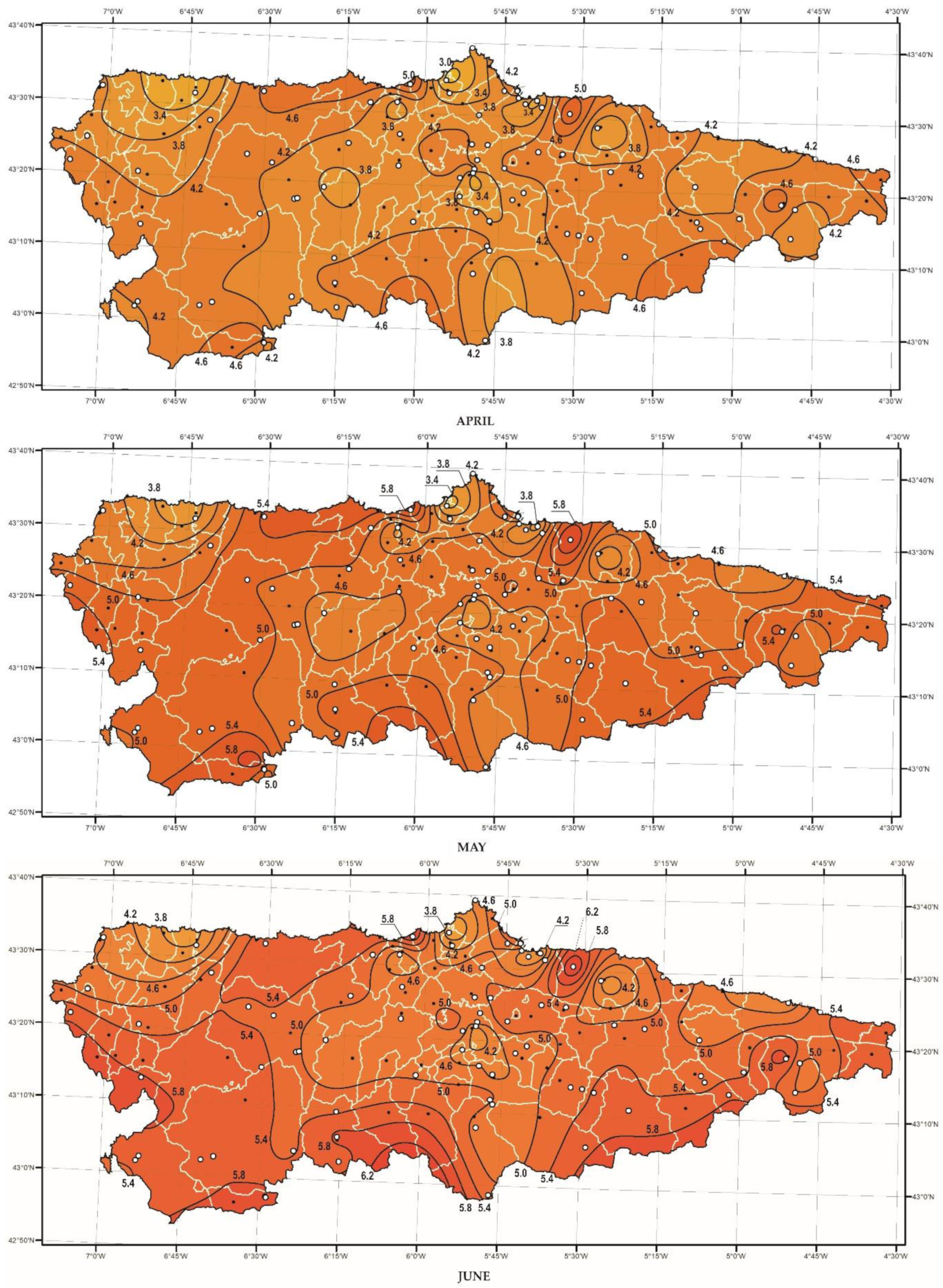
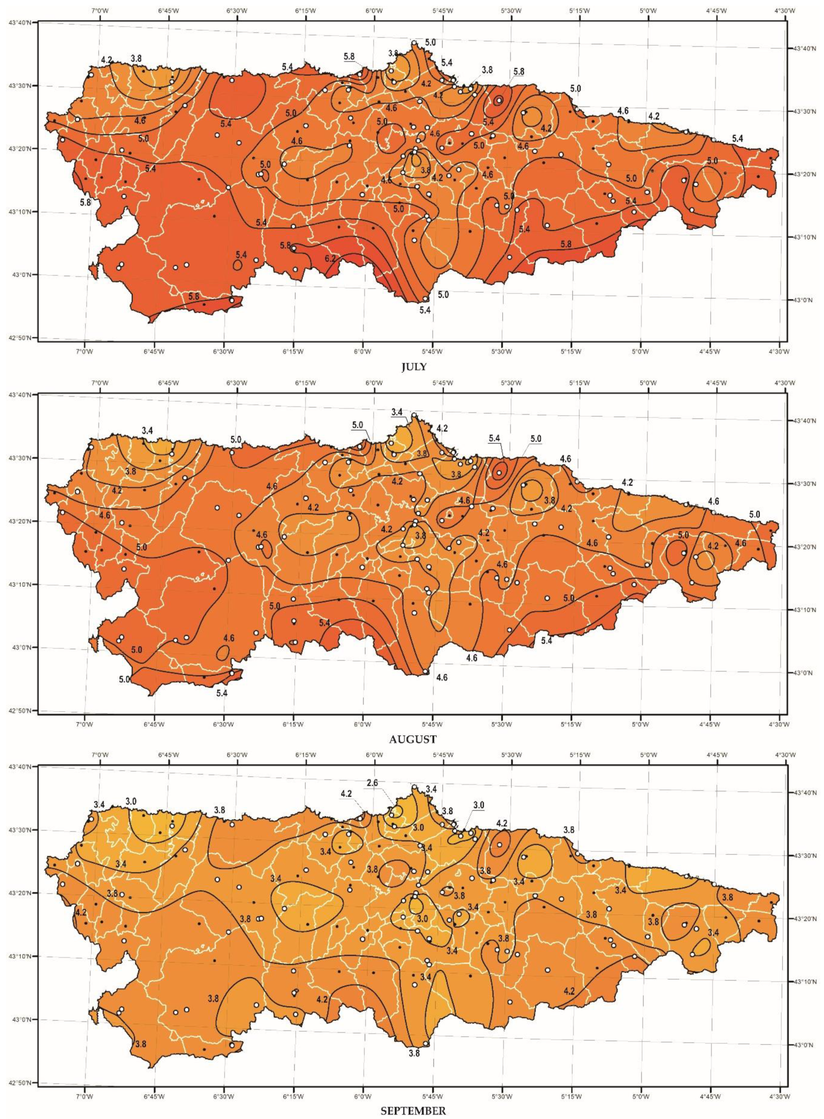
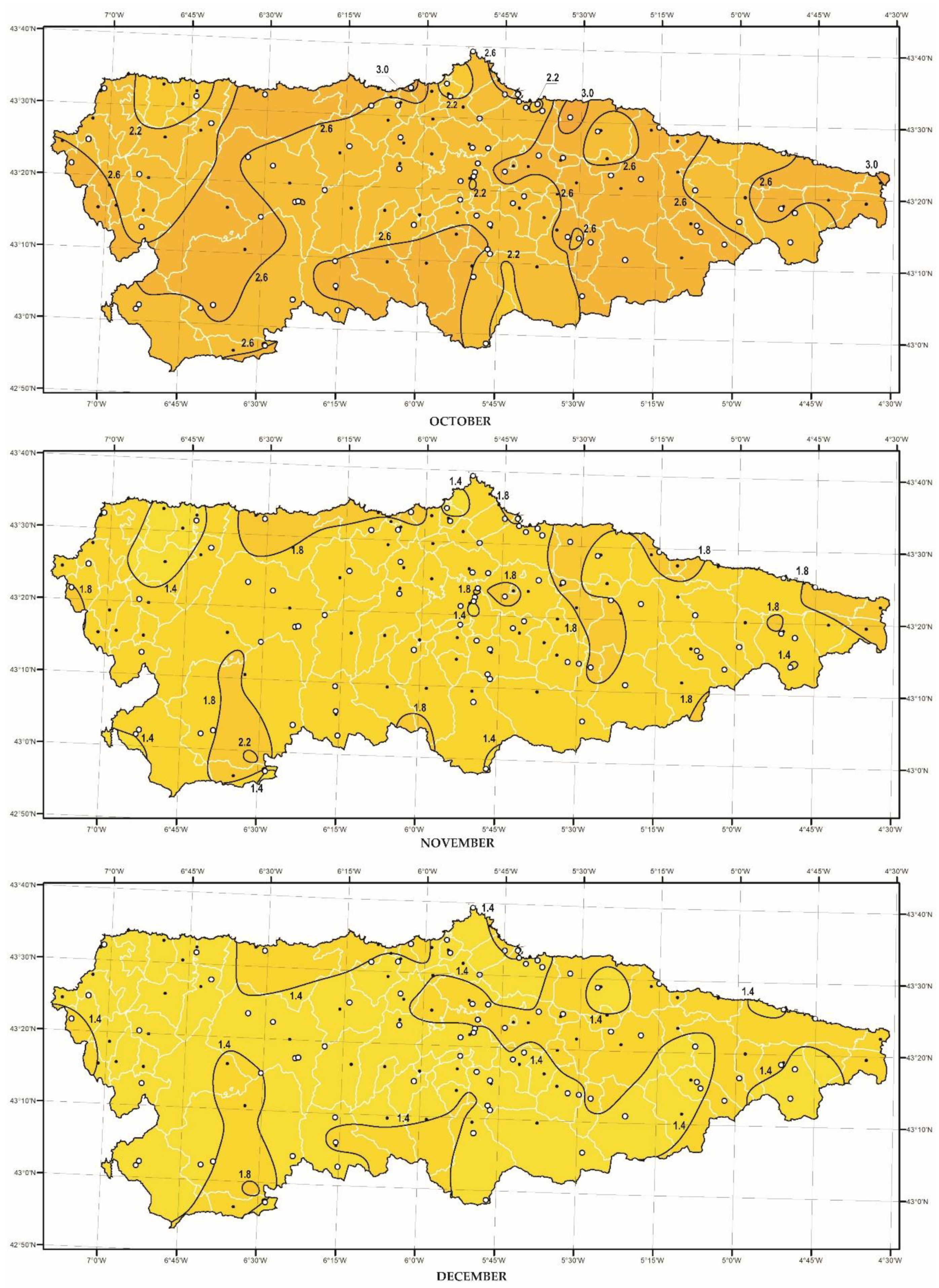
4. Solar Map of Asturias
5. Conclusions
Author Contributions
Funding
Institutional Review Board Statement
Informed Consent Statement
Data Availability Statement
Conflicts of Interest
Nomenclature
| Empirical parameter | |
| Degree-days () | |
| Centred pattern RMSE (kWh/m2) | |
| Normalised centred pattern RMSE | |
| H | Global solar irradiation on horizontal surface (kWh/m2) |
| Extraterrestrial global solar irradiation on horizontal surface (kWh/m2) | |
| KGCC | Köppen-Geiger climate classification |
| L | Distance to the sea (m) |
| MBE | Mean bias error (kWh/m2) |
| NMBE | Normalised mean bias error |
| NRMSE | Normalised root mean square error |
| NSE | Nash-Sutcliffe model efficiency |
| Observed value | |
| Coefficient of determination | |
| RMSE | Root mean square error (kWh/m2) |
| RMBE | Relative mean bias error |
| RRMSE | Relative root mean square error |
| Maximum theoretical duration of sunshine (h) | |
| Actual duration of sunshine (h) | |
| Simulated value | |
| Mean air temperature (K) | |
| Maximum air temperature (K) | |
| Minimum air temperature (K) | |
| z | Elevation above sea level (m) |
| Temperature difference (K) | |
| Latitude (rad) | |
| Longitude (rad) | |
| Standard deviation of experimental solar irradiation (kWh/m2) | |
| Standard deviation of simulated solar irradiation (kWh/m2) | |
| Normalised standard deviation |
Appendix A


References
- Behar, O.; Khellaf, A.; Mohammedi, K. Comparison of solar radiation models and their validation under Algerian climate—The case of direct irradiance. Energy Convers. Manag. 2015, 98, 236–251. [Google Scholar] [CrossRef]
- Muneer, T.; Younes, S.; Munawwar, S. Discourses on solar radiation modeling. Renew. Sustain. Energy Rev. 2007, 11, 551–602. [Google Scholar] [CrossRef]
- Thornton, P.E.; Running, S.W. An improved algorithm for estimating incident daily solar radiation from measurements of temperature, humidity, and precipitation. Agric. Forest Meteorol. 1999, 93, 211–228. [Google Scholar] [CrossRef]
- Zang, H.X.; Xu, Q.S.; Bian, H.H. Generation of typical solar radiation data for different climates of China. Energy 2012, 38, 236–248. [Google Scholar] [CrossRef]
- Antoñanzas, F.; Sanz, A.; Martínez-de-Pisón, F.J.; Perpiñán, O. Evaluation and improvement of empirical models of global solar irradiation: Case study northern Spain. Renew. Energy 2013, 60, 604–614. [Google Scholar] [CrossRef] [Green Version]
- Chen, J.L.; He, L.; Yang, H.; Ma, M.; Chen, Q.; Wu, S.J.; Xiao, Z.L. Empirical models for estimating monthly global solar radiation: A most comprehensive review and comparative case study in China. Renew. Sustain. Energy Rev. 2019, 108, 91–111. [Google Scholar] [CrossRef]
- Abraha, M.G.; Savage, M.J. Comparison of estimates of daily solar radiation from air temperature range for application in crop simulations. Agr. Forest Meteorol. 2008, 148, 401–416. [Google Scholar] [CrossRef]
- Myers, D.R. Solar radiation modeling and measurements for renewable energy applications: Data and model quality. Energy 2005, 30, 1517–1531. [Google Scholar] [CrossRef]
- Prieto, J.I.; García, D. Global solar radiation models: A critical review from the point of view of homogeneity and case study. Renew. Sustain. Energy Rev. 2022, 155, 111856. [Google Scholar] [CrossRef]
- Elagib, N.; Mansell, M.G. New approaches for estimating global solar radiation across Sudan. Energy Convers. Manag. 2000, 41, 419–434. [Google Scholar] [CrossRef]
- Jin, Z.; Yezhen, W.; Gang, Y. General formula for estimation of monthly average daily global solar radiation in China. Energy Convers. Manag. 2005, 46, 57–268. [Google Scholar] [CrossRef]
- Chen, R.; Kang, E.; Ji, X.; Yang, J.; Zhang, Z. Trends of the global radiation and sunshine hours in 1961–1998 and their relationships in China. Energy Convers. Manag. 2006, 47, 2859–2866. [Google Scholar] [CrossRef]
- Robaa, S.M. Validation of the existing models for estimating global solar radiation over Egypt. Energy Convers. Manag. 2009, 50, 184–193. [Google Scholar] [CrossRef]
- Paulescu, M.; Stefu, N.; Calinoiu, D.; Paulescu, E.; Pop, N.; Boata, R.; Mares, O. Ångström–Prescott equation: Physical basis, empirical models and sensitivity analysis. Renew. Sustain. Energy Rev. 2016, 62, 495–506. [Google Scholar] [CrossRef]
- Annandale, J.G.; Jovanovic, N.Z.; Benadé, N.; Allen, R.G. Software for missing data error analysis of Penman–Monteith reference evapotranspiration. Irrig. Sci. 2002, 21, 57–67. [Google Scholar]
- Prieto, J.I.; Martínez-García, J.C.; García, D. Correlation between global solar irradiation and air temperature in Asturias, Spain. Sol. Energy 2009, 83, 1076–1085. [Google Scholar] [CrossRef]
- Prieto, J.I.; Martínez, J.C.; García, D.; Santoro, R.; Rodríguez, A. Solar Map of Asturias; Consorcio de Empresas ARFRISOL: Gijón, Spain, 2009; p. 197. (In Spanish) [Google Scholar]
- Hargreaves, G.H.; Samani, Z.A. Estimating potential evapotranspiration. J. Irrig. Drain. Eng. ASCE 1982, 108, 225–230. [Google Scholar] [CrossRef]
- Hargreaves, G.H. Simplified Coefficients for Estimating Monthly Solar Radiation in North America and Europe; Dept. Paper, Dept. Biol. and Irrig. Engrg.; Utah State University: Logan, UT, USA, 1994. [Google Scholar]
- Meza, F.; Varas, E. Estimation of mean monthly solar global radiation as a function of temperature. Agric. Forest Meteorol. 2000, 100, 231–241. [Google Scholar] [CrossRef]
- Bristow, K.L.; Campbell, G.S. On the relationship between incoming solar radiation and daily maximum and minimum temperature. Agr. Forest Meteorol. 1984, 31, 159–166. [Google Scholar] [CrossRef]
- Weiss, A.; Hays, C.J.; Hu, Q.; Easterling, W.E. Incorporating bias error in calculating solar irradiance: Implications for crop yield simulations. Agron. J. 2001, 93, 1321–1326. [Google Scholar] [CrossRef]
- Goodin, D.G.; Hutchinson, J.M.S.; Vanderlip, R.L.; Knapp, M.C. Estimating solar irradiance for crop modeling using daily air temperature data. Agron. J. 1999, 91, 845–851. [Google Scholar] [CrossRef]
- Bandyopadhyay, A.; Bhadra, A.; Raghuwanshi, N.S.; Singh, R. Estimation of monthly solar radiation from measured air temperature extremes. Agric. Forest Meteorol. 2008, 148, 1707–1718. [Google Scholar] [CrossRef]
- Allen, R.G. Evaluation of Procedures for Estimating Mean Monthly Solar Radiation from Air Temperature; Technical Report; United Nations Food and Agric. Org. (FAO): Rome, Italy, 1995. [Google Scholar]
- Hargreaves, G.L.; Hargreaves, G.H.; Riley, J.P. Irrigation water requirements for Senegal River Basin. J. Irrig. Drain. Eng. 1985, 111, 265–275. [Google Scholar] [CrossRef]
- Supit, I.; van Kappel, R.R. A simple method to estimate global radiation. Sol. Energy 1998, 63, 147–160. [Google Scholar] [CrossRef]
- Hunt, L.A.; Kucharb, L.; Swanton, C.J. Estimation of solar radiation for use in crop modeling. Agric. Forest Meteorol. 1998, 91, 293–300. [Google Scholar] [CrossRef]
- Chen, R.; Ersi, K.; Yang, J.; Lu, S.; Zhao, W. Validation of five global radiation models with measured daily data in China. Energy Convers. Manag. 2004, 45, 1759–1769. [Google Scholar] [CrossRef]
- Pandey, C.K.; Katiyar, A.K. Temperature base correlation for the estimation of global solar radiation on horizontal surface. Int. J. Energy Environ. 2010, 1, 737–744. [Google Scholar]
- Chen, J.L.; Li, G.S. Estimation of monthly average daily solar radiation from measured meteorological data in Yangtze River Basin in China. Int. J. Climatol. 2013, 33, 487–498. [Google Scholar] [CrossRef]
- Richardson, C.W. Weather simulation for crop management models. Trans. ASAE 1985, 28, 1602–1606. [Google Scholar] [CrossRef]
- Li, M.; Liu, H.; Guo, P.; Wu, W. Estimation of daily solar radiation from routinely observed meteorological data in Chongqing, China. Energy Convers. Manag. 2010, 51, 2575–2579. [Google Scholar] [CrossRef]
- Hassan, G.E.; Youssef, M.E.; Mohamed, Z.E.; Ali, M.A.; Hanafy, A.A. New Temperature-based Models for Predicting Global Solar Radiation. Appl. Energy 2016, 179, 437–450. [Google Scholar] [CrossRef]
- Chazarra, A.; Flórez, E.; Peraza, B.; Tohá, T.; Lorenzo, B.; Criado, E.; Moreno, J.V.; Romero, R.; Botey, R. Mapas Climáticos de España (1981–2010) y ETo (1996–2016); AEMET: Madrid, Spain, 2018; (In Spanish). [Google Scholar] [CrossRef]
- Lewis, C. International and Business Forecasting Methods; Butterworths: London, UK, 1982; p. 143. [Google Scholar]
- Gueymard, C.A. A review of validation methodologies and statistical performance indicators for modeled solar radiation data: Towards a better bankability of solar projects. Renew. Sustain. Energy Rev. 2014, 39, 1024–1034. [Google Scholar] [CrossRef]
- Taylor, K.E. Summarizing multiple aspects of model performance in a single diagram. J. Geophys. Res. 2001, 106, 7183–7192. [Google Scholar] [CrossRef]
- Soutullo, S.; Giancola, E.; Sánchez, M.N.; Ferrer, J.A.; García, D.; Súarez, M.J.; Prieto, J.I.; Antuña-Yudego, E.; Carús, J.L.; Fernández, M.A.; et al. Methodology for Quantifying the Energy Saving Potentials Combining Building Retrofitting, Solar Thermal Energy and Geothermal Resources. Energy 2020, 13, 5970. [Google Scholar] [CrossRef]
- Mirzabe, A.H.; Hajiahmad, A.; Keyhani, A.; Mirzaei, N. Approximation of daily solar radiation: A comprehensive review on employing of regression models. Renew. Energy Focus 2022, 41, 143–159. [Google Scholar] [CrossRef]
- ArcGIS Desktop 9.3 Service Pack 1, ESRI. 2008.
- Royal Decree 314/2006, Approved 17th May, in which Technical Building Code for Spain is Approved. Available online: https://www.global-regulation.com/translation/spain/1446654/royal-decree-314-2006%252c-of-march-17%252c-which-approves-the-technical-building-code.html (accessed on 11 May 2022).
- Vázquez, M.; Santos, J.M.; Prado, M.T.; Vázquez, D.; Rodrigues, F.M. Atlas de Radiación Solar de Galicia; Universidad de Vigo: Vigo, Spain, 2005; Available online: https://www.meteogalicia.gal/datosred/infoweb/meteo/docs/publicacions/libros/Atlas_Radiacion_Solar_Galicia.pdf (accessed on 11 May 2022).
- Attia, S.; Lacombe, T.; Rakotondramiarana, H.T.; Garde, F.; Roshan, G.R. Analysis tool for bioclimatic design strategies in hot humid climates. Sustain. Cities Soc. 2019, 45, 8–24. [Google Scholar] [CrossRef] [Green Version]
- Praene, J.P.; Malet-Damour, B.; Radanielina, M.H.; Fontaine, L.; Rivière, G. GIS-based approach to identify climatic zoning: A hierarchical clustering on principal component analysis. Build. Environ. 2019, 164, 106330. [Google Scholar] [CrossRef] [Green Version]
- Dailidé, R.; Povilanskas, R.; Méndez, J.A.; Simanavičiūtė, G. A new approach to local climate identification in the Baltic Sea’s coastal area. Baltica 2019, 32, 210–218. [Google Scholar] [CrossRef]
- Sánchez, F.J.; Salmerón, J.M.; Domínguez, S.A. A new methodology towards determining building performance under modified outdoor conditions. Build. Environ. 2006, 41, 1231–1238. [Google Scholar]
- Sánchez, F.J.; Domínguez, S.A.; Molina, J.M.; González, R. Climatic zoning and its application to Spanish building energy performance regulations. Energy Build. 2008, 40, 1984–1990. [Google Scholar]
- Salmerón, J.M.; Álvarez, S.; Molina, J.L.; Ruiz, A.; Sánchez, F.J. Tightening the energy consumptions of buildings depending on their typology and on Climate Severity Indexes. Energy Build. 2013, 58, 372–377. [Google Scholar] [CrossRef]
- Ögelman, H.; Ecevit, A.; Tasemiroglu, E. A new method for estimating solar radiation from bright sunshine data. Sol. Energy 1984, 33, 619–625. [Google Scholar] [CrossRef]


| Station No. | Location | Region | KGCC | Period | |||||
|---|---|---|---|---|---|---|---|---|---|
| (°) | (°) | (m) | (km) | (m/km) | |||||
| 1 | Avilés a | Asturias | Cfb | 43.584 | −5.918 | 12 | 1.6 | 7.56 | 2003–2016 |
| 2 | Oviedo b | “ | Cfb | 43.354 | −5.873 | 350 | 25.7 | 13.61 | 2003–2016 |
| 3 | Oviedo a | “ | Cfb | 43.371 | −5.836 | 189 | 22.8 | 8.30 | 2003–2016 |
| 4 | Mieres a | “ | Cfb | 43.258 | −5.773 | 206 | 32.8 | 6.29 | 2003–2016 |
| 5 | Langreo a | “ | Cfb | 43.309 | −5.706 | 247 | 26.3 | 9.38 | 2003–2016 |
| 6 | Gijón a | “ | Cfb | 43.531 | −5.672 | 32 | 1.4 | 22.34 | 2003–2016 |
| 7 | Niembro c | “ | Cfb | 43.439 | −4.850 | 136 | 0.4 | 376.65 | 2003–2016 |
| 8 | Santander-CMT b | Cantabria | Cfb | 43.491 | −3.801 | 60 | 0.2 | 333.33 | 2003–2016 |
| 9 | A Coruña b | Galicia | Csb | 43.366 | −8.421 | 60 | 0.7 | 85.71 | 1985–2016 |
| 10 | Santiago b | “ | Cfb | 42.888 | −8.411 | 372 | 40.9 | 9.10 | 1985–2016 |
| 11 | A Coruña-Airport b | “ | Csb | 43.304 | −8.378 | 100 | 4.1 | 24.59 | 2004–2016 |
| 12 | Lugo b | “ | Csb | 43.115 | −7.456 | 446 | 50.8 | 8.78 | 1985–1989 |
| 13 | Oviedo b | Asturias | Cfb | 43.354 | −5.873 | 350 | 25.7 | 13.61 | 1975–2016 |
| 14 | Gijón d | “ | Cfb | 43.545 | −5.693 | 13 | 0.3 | 42.85 | 1993–2005 |
| 15 | Santander-Centre b | Cantabria | Cfb | 43.491 | −3.819 | 72 | 1.1 | 63.52 | 1989–1997 |
| 16 | Bilbao b | Basque Country | Cfb | 43.298 | −2.906 | 44 | 9.5 | 4.63 | 1985–2016 |
| 17 | Vitoria (II) b | “ | Cfb | 42.882 | −2.735 | 513 | 54.2 | 9.46 | 2011–2016 |
| 18 | Vitoria(I) b | “ | Cfb | 42.884 | −2.723 | 508 | 55.3 | 9.19 | 2000–2008 |
| 19 | San Sebastián b | “ | Cfb | 43.306 | −2.041 | 263 | 1.1 | 239.09 | 1983–2016 |
| 20 | Pamplona b | Navarra | Cfb | 42.777 | −1.650 | 461 | 66.0 | 6.98 | 2006–2008 |
| 21 | Girona b | Catalonia | Csa | 41.912 | +2.763 | 145 | 24.7 | 5.87 | 2003–2008 |
| No. | Location | Jan | Feb | Mar | Apr | May | Jun | Jul | Aug | Sep | Oct | Nov | Dec | Annual | |
|---|---|---|---|---|---|---|---|---|---|---|---|---|---|---|---|
| 1 | Avilés | 13.77 | 13.44 | 15.01 | 16.12 | 17.88 | 20.54 | 22.48 | 23.08 | 22.03 | 19.62 | 16.57 | 14.75 | 17.94 | 3.35 |
| 2 | Oviedo | 11.90 | 12.14 | 14.80 | 16.43 | 18.39 | 21.52 | 23.22 | 24.01 | 22.59 | 19.56 | 14.41 | 12.34 | 17.61 | 4.35 |
| 3 | Oviedo | 12.53 | 12.38 | 14.56 | 16.10 | 18.04 | 21.08 | 22.62 | 23.60 | 22.24 | 19.52 | 14.63 | 12.68 | 17.50 | 4.04 |
| 4 | Mieres | 12.68 | 13.06 | 16.00 | 17.36 | 19.41 | 22.74 | 24.65 | 25.54 | 24.10 | 20.85 | 15.39 | 13.05 | 18.74 | 4.59 |
| 5 | Langreo | 14.26 | 13.92 | 16.35 | 17.97 | 20.45 | 23.70 | 25.28 | 26.07 | 24.55 | 21.72 | 16.76 | 15.32 | 19.70 | 4.29 |
| 6 | Gijón | 12.71 | 12.75 | 14.30 | 15.16 | 17.18 | 20.09 | 22.07 | 22.81 | 21.57 | 19.39 | 15.20 | 13.34 | 17.22 | 3.64 |
| 7 | Niembro | 12.09 | 11.34 | 12.73 | 13.55 | 15.24 | 17.92 | 19.83 | 20.78 | 19.55 | 18.08 | 14.49 | 12.81 | 15.70 | 3.21 |
| 8 | Santander-CMT | 13.13 | 12.66 | 14.51 | 15.88 | 17.54 | 20.44 | 22.50 | 23.36 | 22.06 | 20.26 | 16.00 | 13.86 | 17.68 | 3.71 |
| 9 | A Coruña | 13.50 | 14.08 | 15.62 | 16.31 | 18.44 | 20.69 | 22.33 | 23.00 | 22.14 | 19.48 | 16.00 | 14.34 | 17.99 | 3.32 |
| 10 | Santiago | 11.20 | 12.25 | 14.78 | 16.05 | 18.54 | 22.13 | 24.33 | 24.68 | 22.93 | 18.28 | 13.97 | 11.92 | 17.59 | 4.75 |
| 11 | A Coruña-Airport | 13.43 | 13.65 | 15.64 | 17.35 | 19.11 | 22.05 | 23.62 | 23.95 | 23.32 | 20.58 | 16.05 | 14.33 | 18.59 | 3.86 |
| 12 | Lugo | 10.45 | 11.73 | 14.65 | 13.95 | 18.74 | 21.14 | 23.80 | 24.88 | 24.48 | 19.30 | 13.78 | 12.08 | 17.41 | 5.06 |
| 13 | Oviedo | 11.82 | 12.68 | 14.77 | 15.53 | 17.99 | 20.77 | 22.74 | 23.27 | 22.08 | 18.85 | 14.47 | 12.47 | 17.29 | 4.03 |
| 14 | Gijón | 14.80 | 14.80 | 15.30 | 16.30 | 17.90 | 20.50 | 22.40 | 23.50 | 22.10 | 19.60 | 16.10 | 14.60 | 18.16 | 3.17 |
| 15 | Santander-Centre | 13.60 | 14.50 | 15.80 | 15.30 | 19.20 | 20.70 | 23.40 | 24.10 | 21.80 | 19.50 | 16.40 | 14.20 | 18.21 | 3.56 |
| 16 | Bilbao | 13.69 | 14.19 | 16.58 | 17.80 | 20.99 | 23.42 | 25.45 | 26.34 | 24.74 | 21.73 | 16.57 | 14.18 | 19.64 | 4.49 |
| 17 | Vitoria (II) | 9.94 | 8.88 | 13.66 | 16.06 | 19.10 | 24.08 | 27.08 | 27.54 | 24.67 | 20.17 | 13.27 | 10.15 | 17.88 | 6.55 |
| 18 | Vitoria (I) | 9.11 | 10.59 | 14.17 | 15.97 | 20.07 | 24.74 | 25.89 | 25.96 | 23.18 | 18.86 | 12.18 | 9.04 | 17.48 | 6.24 |
| 19 | San Sebastián | 11.08 | 11.43 | 13.38 | 14.73 | 17.73 | 19.98 | 21.86 | 22.64 | 21.21 | 18.74 | 14.11 | 11.91 | 16.57 | 4.10 |
| 20 | Pamplona | 10.04 | 11.12 | 14.53 | 18.30 | 21.24 | 25.63 | 28.82 | 29.54 | 25.64 | 20.94 | 13.88 | 10.12 | 19.15 | 6.90 |
| 21 | Girona | 13.72 | 14.21 | 16.93 | 19.69 | 23.50 | 28.54 | 31.24 | 30.93 | 27.07 | 22.91 | 17.31 | 13.99 | 21.67 | 6.34 |
| No. | Location | Jan | Feb | Mar | Apr | May | Jun | Jul | Aug | Sep | Oct | Nov | Dec | Annual | |
|---|---|---|---|---|---|---|---|---|---|---|---|---|---|---|---|
| 1 | Avilés | 7.87 | 7.15 | 8.51 | 10.33 | 12.28 | 15.07 | 17.08 | 17.20 | 15.82 | 12.89 | 10.28 | 7.96 | 11.87 | 3.56 |
| 2 | Oviedo | 4.82 | 4.35 | 5.99 | 7.66 | 9.79 | 12.96 | 14.73 | 14.86 | 13.34 | 10.86 | 7.21 | 5.05 | 9.30 | 3.80 |
| 3 | Oviedo | 5.24 | 4.87 | 6.41 | 8.34 | 10.46 | 13.62 | 15.38 | 15.39 | 13.72 | 10.98 | 7.47 | 4.86 | 9.73 | 3.90 |
| 4 | Mieres | 3.80 | 3.66 | 5.63 | 7.80 | 10.26 | 13.82 | 15.70 | 15.71 | 13.80 | 10.71 | 6.46 | 3.58 | 9.24 | 4.51 |
| 5 | Langreo | 4.80 | 4.25 | 6.01 | 7.96 | 10.30 | 13.65 | 15.36 | 15.44 | 13.64 | 10.76 | 7.07 | 4.42 | 9.47 | 4.10 |
| 6 | Gijón | 6.58 | 6.09 | 7.62 | 9.49 | 11.65 | 14.87 | 16.84 | 17.00 | 15.41 | 12.55 | 9.12 | 6.73 | 11.16 | 3.94 |
| 7 | Niembro | 7.73 | 6.88 | 8.23 | 9.49 | 11.41 | 14.39 | 16.30 | 16.78 | 15.69 | 13.59 | 10.27 | 8.44 | 11.60 | 3.44 |
| 8 | Santander-CMT | 7.96 | 7.11 | 8.58 | 10.04 | 12.14 | 15.15 | 17.00 | 17.54 | 16.10 | 13.93 | 10.71 | 8.59 | 12.07 | 3.60 |
| 9 | A Coruña | 8.22 | 8.13 | 9.21 | 10.01 | 12.17 | 14.40 | 16.03 | 16.47 | 15.36 | 13.20 | 10.52 | 9.08 | 11.90 | 2.98 |
| 10 | Santiago | 4.06 | 4.17 | 5.28 | 6.21 | 8.41 | 11.15 | 12.92 | 13.14 | 11.96 | 9.62 | 6.59 | 5.06 | 8.21 | 3.29 |
| 11 | A Coruña-Airport | 6.29 | 4.97 | 6.59 | 8.05 | 10.14 | 13.08 | 14.68 | 14.54 | 13.04 | 11.25 | 8.15 | 6.14 | 9.74 | 3.35 |
| 12 | Lugo | 1.33 | 1.83 | 2.63 | 4.30 | 6.88 | 9.40 | 12.12 | 10.86 | 9.78 | 7.18 | 4.06 | 3.26 | 6.13 | 3.58 |
| 13 | Oviedo | 4.54 | 4.73 | 5.95 | 6.84 | 9.39 | 12.32 | 14.36 | 14.69 | 13.16 | 10.49 | 7.15 | 5.37 | 9.08 | 3.66 |
| 14 | Gijón | 8.18 | 8.16 | 9.26 | 10.20 | 12.80 | 15.80 | 17.60 | 18.30 | 16.70 | 13.70 | 9.81 | 8.01 | 12.38 | 3.77 |
| 15 | Santander-Centre | 7.50 | 7.70 | 9.00 | 9.00 | 12.50 | 14.60 | 17.20 | 17.80 | 15.20 | 12.90 | 10.50 | 8.70 | 11.88 | 3.52 |
| 16 | Bilbao | 5.28 | 5.08 | 6.48 | 7.86 | 10.82 | 13.53 | 15.55 | 15.86 | 13.87 | 11.61 | 8.17 | 6.04 | 10.01 | 3.86 |
| 17 | Vitoria (II) | 1.92 | 0.68 | 2.60 | 4.76 | 6.98 | 10.32 | 12.60 | 12.30 | 10.47 | 7.43 | 4.85 | 2.32 | 6.44 | 4.04 |
| 18 | Vitoria (I) | 1.37 | 1.29 | 2.93 | 4.48 | 7.26 | 10.94 | 11.96 | 12.38 | 9.90 | 8.29 | 3.85 | 1.49 | 6.34 | 4.10 |
| 19 | San Sebastián | 5.91 | 5.77 | 7.26 | 8.37 | 11.11 | 13.86 | 16.06 | 16.54 | 14.81 | 12.54 | 8.84 | 6.84 | 10.66 | 3.83 |
| 20 | Pamplona | 1.64 | 1.72 | 3.57 | 6.27 | 8.77 | 12.21 | 14.55 | 14.73 | 12.39 | 9.16 | 5.57 | 1.65 | 7.69 | 4.78 |
| 21 | Girona | 1.19 | 1.28 | 4.08 | 7.01 | 10.21 | 14.73 | 17.22 | 17.10 | 14.29 | 11.09 | 5.56 | 1.80 | 8.80 | 5.86 |
| No. | Location | Jan | Feb | Mar | Apr | May | Jun | Jul | Aug | Sep | Oct | Nov | Dec | Annual | |
|---|---|---|---|---|---|---|---|---|---|---|---|---|---|---|---|
| 1 | Avilés | 1.146 | 1.837 | 2.463 | 3.269 | 3.880 | 4.005 | 3.907 | 3.547 | 2.827 | 2.015 | 1.294 | 1.204 | 2.616 | 1.058 |
| 2 | Oviedo | 1.461 | 2.216 | 3.343 | 4.232 | 4.770 | 5.012 | 5.088 | 4.768 | 3.991 | 2.693 | 1.650 | 1.433 | 3.388 | 1.379 |
| 3 | Oviedo | 1.257 | 2.046 | 3.098 | 4.113 | 4.672 | 4.943 | 4.783 | 4.586 | 3.756 | 2.598 | 1.624 | 1.261 | 3.228 | 1.369 |
| 4 | Mieres | 1.360 | 2.038 | 2.874 | 3.496 | 3.937 | 4.118 | 4.083 | 4.025 | 3.490 | 2.374 | 1.477 | 1.263 | 2.878 | 1.081 |
| 5 | Langreo | 1.452 | 2.083 | 2.827 | 3.846 | 4.098 | 4.432 | 4.205 | 3.951 | 3.483 | 2.534 | 1.659 | 1.381 | 2.996 | 1.098 |
| 6 | Gijón | 1.303 | 1.869 | 2.555 | 3.093 | 3.441 | 3.629 | 3.836 | 3.748 | 3.203 | 2.371 | 1.513 | 1.375 | 2.661 | 0.918 |
| 7 | Niembro | 1.364 | 2.122 | 3.230 | 4.201 | 4.878 | 4.855 | 4.932 | 4.605 | 3.861 | 2.604 | 1.543 | 1.357 | 3.296 | 1.381 |
| 8 | Santander-CMT | 1.331 | 2.186 | 3.420 | 4.609 | 5.452 | 5.796 | 5.651 | 5.170 | 4.213 | 2.815 | 1.599 | 1.315 | 3.630 | 1.667 |
| 9 | A Coruña | 1.404 | 2.244 | 3.500 | 4.565 | 5.463 | 6.153 | 6.213 | 5.456 | 4.198 | 2.642 | 1.605 | 1.239 | 3.723 | 1.791 |
| 10 | Santiago | 1.293 | 2.148 | 3.062 | 4.020 | 4.776 | 5.444 | 5.383 | 4.994 | 4.031 | 2.569 | 1.541 | 1.165 | 3.369 | 1.543 |
| 11 | A Coruña-Airport | 1.326 | 2.227 | 3.402 | 4.822 | 5.464 | 5.848 | 6.155 | 5.453 | 4.228 | 2.804 | 1.621 | 1.272 | 3.719 | 1.762 |
| 12 | Lugo | 1.408 | 2.069 | 3.388 | 3.726 | 5.067 | 5.794 | 5.904 | 5.421 | 4.180 | 2.731 | 1.797 | 1.399 | 3.574 | 1.633 |
| 13 | Oviedo | 1.490 | 2.199 | 3.306 | 4.143 | 4.487 | 4.899 | 4.825 | 4.413 | 3.734 | 2.572 | 1.641 | 1.350 | 3.255 | 1.290 |
| 14 | Gijón | 1.639 | 2.245 | 3.341 | 4.131 | 4.614 | 4.635 | 4.636 | 4.375 | 3.905 | 2.566 | 1.791 | 1.501 | 3.282 | 1.205 |
| 15 | Santander-Centre | 1.431 | 2.178 | 3.306 | 4.085 | 5.157 | 5.262 | 5.352 | 4.497 | 3.693 | 2.455 | 1.475 | 1.119 | 3.334 | 1.507 |
| 16 | Bilbao | 1.318 | 2.033 | 3.094 | 3.946 | 4.847 | 5.141 | 5.116 | 4.690 | 3.691 | 2.464 | 1.429 | 1.173 | 3.245 | 1.467 |
| 17 | Vitoria (II) | 1.352 | 2.190 | 3.223 | 4.540 | 4.933 | 5.798 | 5.761 | 5.106 | 4.037 | 2.695 | 1.310 | 1.303 | 3.521 | 1.660 |
| 18 | Vitoria (I) | 1.428 | 2.139 | 3.279 | 4.162 | 5.154 | 5.772 | 5.952 | 5.065 | 4.114 | 2.632 | 1.610 | 1.233 | 3.545 | 1.654 |
| 19 | San Sebastián | 1.329 | 2.063 | 3.290 | 4.235 | 4.896 | 5.384 | 5.284 | 4.632 | 3.895 | 2.561 | 1.516 | 1.200 | 3.357 | 1.510 |
| 20 | Pamplona | 1.473 | 2.419 | 3.590 | 4.400 | 5.549 | 5.943 | 6.768 | 5.507 | 4.239 | 2.963 | 1.699 | 1.354 | 3.825 | 1.788 |
| 21 | Girona | 1.815 | 2.712 | 3.497 | 4.745 | 5.664 | 6.407 | 6.164 | 5.139 | 4.270 | 2.913 | 1.980 | 1.640 | 3.912 | 1.648 |
| Station\Model | No.1 | No.2 | No.3 | No.4 | No.5 | No.6 | No.7 | No.8 | No.9 | No.10 | No.11 | No.12 | No.13 | |
|---|---|---|---|---|---|---|---|---|---|---|---|---|---|---|
| No.1 | 0.142 | 0.017 | 0.076 | 0.142 | 2.397 | 0.221 | 0.236 | −2.245 | 0.284 | 0.603 | 2248 | 0.239 | 0.314 | |
| -- | -- | -- | -- | -- | 0.052 | 0.063 | 2.541 | 0.011 | 0.141 | −4405 | 0.016 | 0.017 | ||
| -- | -- | -- | -- | -- | -- | -- | -- | -- | -- | 2158 | −0.015 | −0.508 | ||
| RRMSE (%) | 4.85 | 10.15 | 40.66 | 4.85 | 5.17 | 4.22 | 4.23 | 4.26 | 4.21 | 4.27 | 3.85 | 3.99 | 4.92 | |
| RMBE (%) | 0.05 | −1.68 | −22.90 | 0.04 | 0.03 | 0.17 | 0.17 | 0.17 | 0.17 | 0.09 | 0.14 | 0.16 | −0.91 | |
| No.2 | 0.156 | 0.013 | 0.080 | 0.156 | 2.623 | −0.053 | −0.071 | −9.460 | 0.193 | 3.911 | 1520 | 0.177 | 0.396 | |
| -- | -- | -- | -- | -- | 0.174 | 0.246 | 9.627 | 0.031 | 0.614 | −2964 | 0.034 | 0.003 | ||
| -- | -- | -- | -- | -- | -- | -- | -- | -- | -- | 1445 | −0.034 | 0.325 | ||
| RRMSE (%) | 3.32 | 7.27 | 21.65 | 3.31 | 3.39 | 3.29 | 3.32 | 3.24 | 3.26 | 3.25 | 3.04 | 3.22 | 6.15 | |
| RMBE (%) | 0.16 | −1.66 | −7.01 | 0.07 | 0.19 | 0.11 | 0.11 | 0.10 | 0.10 | 0.05 | 0.09 | 0.10 | −0.86 | |
| No.3 | 0.152 | 0.014 | 0.070 | 0.152 | 2.561 | −0.353 | −0.375 | −11.688 | 0.037 | 6.476 | 3886 | 0.066 | 0.334 | |
| -- | -- | -- | -- | -- | 0.279 | 0.390 | 11.789 | 0.050 | 0.759 | −7575 | 0.040 | 0.008 | ||
| -- | -- | -- | -- | -- | -- | -- | -- | -- | -- | 3691 | −0.036 | 0.149 | ||
| RRMSE (%) | 6.89 | 6.42 | 34.52 | 6.88 | 7.43 | 6.24 | 6.25 | 7.19 | 6.24 | 7.17 | 6.84 | 4.30 | 7.67 | |
| RMBE (%) | 0.57 | −0.04 | −14.58 | 0.50 | 0.58 | 0.36 | 0.36 | 0.47 | 0.36 | 0.24 | 0.43 | 0.18 | −0.40 | |
| No.4 | 0.126 | 0.008 | 0.043 | 0.126 | 2.111 | −0.372 | −0.471 | −10.683 | 0.009 | 9.244 | −1181 | 0.010 | 0.353 | |
| -- | -- | -- | -- | -- | 0.246 | 0.381 | 10.709 | 0.040 | 0.936 | 2275 | 0.040 | 0.236 | ||
| -- | -- | -- | -- | -- | -- | -- | -- | -- | -- | −1095 | −0.040 | −1.647 | ||
| RRMSE (%) | 3.95 | 3.67 | 30.40 | 3.94 | 3.98 | 2.96 | 2.95 | 3.19 | 2.96 | 3.19 | 3.08 | 2.94 | 6.97 | |
| RMBE (%) | 0.31 | −0.37 | −14.58 | 0.24 | 0.30 | 0.09 | 0.09 | 0.10 | 0.09 | 0.05 | 0.09 | 0.09 | −2.06 | |
| No.5 | 0.127 | 0.007 | 0.038 | 0.127 | 2.132 | −0.074 | −0.146 | −8.298 | 0.163 | 4.759 | 2346 | 0.118 | 0.400 | |
| -- | -- | -- | -- | -- | 0.150 | 0.237 | 8.399 | 0.024 | 0.742 | −4535 | 0.030 | 1388 | ||
| -- | -- | -- | -- | -- | -- | -- | -- | -- | -- | 2191 | −0.033 | −6.048 | ||
| RRMSE (%) | 4.65 | 5.83 | 29.28 | 4.65 | 4.33 | 4.64 | 4.66 | 4.16 | 4.62 | 4.16 | 3.94 | 3.78 | 5.30 | |
| RMBE (%) | 0.23 | −0.29 | −16.48 | 0.16 | 0.24 | 0.21 | 0.21 | 0.17 | 0.21 | 0.09 | 0.16 | 0.14 | −0.37 | |
| No.6 | 0.149 | 0.018 | 0.086 | 0.149 | 2.517 | −0.238 | −0.176 | −12.152 | 0.063 | 5.754 | −1333 | −0.082 | 0.356 | |
| -- | -- | -- | -- | -- | 0.246 | 0.302 | 12.257 | 0.050 | 0.716 | 2600 | 0.067 | 28390 | ||
| -- | -- | -- | -- | -- | -- | -- | -- | -- | -- | −1267 | −0.063 | −7.145 | ||
| RRMSE (%) | 6.94 | 8.28 | 36.50 | 6.93 | 7.06 | 6.22 | 6.20 | 6.72 | 6.24 | 6.68 | 6.64 | 5.15 | 9.65 | |
| RMBE (%) | 0.75 | −1.19 | −21.39 | 0.72 | 0.71 | 0.39 | 0.38 | 0.45 | 0.39 | 0.22 | 0.43 | 0.28 | −0.86 | |
| No.7 | 0.214 | 0.050 | 0.221 | 0.214 | 3.615 | 0.580 | 0.534 | 6.392 | 0.509 | 0.194 | −4659 | 0.233 | 0.368 | |
| -- | -- | -- | -- | -- | −0.072 | −0.071 | −5.873 | −0.018 | −0.190 | 9196 | 0.030 | 0.004 | ||
| -- | -- | -- | -- | -- | -- | -- | -- | -- | -- | −4537 | −0.023 | 0.297 | ||
| RRMSE (%) | 9.21 | 14.14 | 42.36 | 9.20 | 9.67 | 7.10 | 7.10 | 7.00 | 7.09 | 6.99 | 6.91 | 5.90 | 6.54 | |
| RMBE (%) | 0.33 | −1.61 | −22.50 | 0.21 | 0.29 | 0.48 | 0.48 | 0.47 | 0.48 | 0.24 | 0.45 | 0.34 | −0.87 | |
| No.8 | 0.198 | 0.031 | 0.161 | 0.198 | 3.350 | −0.564 | −0.435 | −21.258 | −0.039 | 21.760 | −11238 | 0.010 | 0.346 | |
| -- | -- | -- | -- | -- | 0.436 | 0.525 | 21.308 | 0.091 | 0.978 | 22015 | 0.063 | 0.005 | ||
| -- | -- | -- | -- | -- | -- | -- | -- | -- | -- | −10781 | −0.055 | 0.445 | ||
| RRMSE (%) | 10.11 | 8.70 | 35.00 | 10.09 | 10.60 | 8.76 | 8.69 | 9.98 | 8.82 | 9.84 | 9.44 | 5.84 | 6.63 | |
| RMBE (%) | 1.15 | 1.04 | −12.00 | 1.06 | 1.17 | 0.77 | 0.76 | 0.96 | 0.78 | 0.48 | 0.87 | 0.36 | −0.21 | |
| No.9 | 0.193 | 0.028 | 0.156 | 0.193 | 3.265 | −0.876 | −0.726 | −33.871 | −0.210 | 186.320 | −3811 | −0.112 | 0.346 | |
| -- | -- | -- | -- | -- | 0.548 | 0.666 | 33.628 | 0.113 | 1.553 | 7433 | 0.083 | 0.003 | ||
| -- | -- | -- | -- | -- | -- | -- | -- | -- | -- | −3624 | −0.076 | 0.658 | ||
| RRMSE (%) | 9.46 | 5.35 | 30.53 | 9.45 | 9.89 | 4.67 | 4.66 | 5.46 | 4.68 | 5.47 | 5.40 | 3.76 | 4.38 | |
| RMBE (%) | 1.44 | 1.32 | −6.15 | 1.39 | 1.46 | 0.23 | 0.22 | 0.32 | 0.23 | 0.15 | 0.29 | 0.15 | −0.22 | |
| No.10 | 0.142 | 0.009 | 0.068 | 0.142 | 2.381 | −0.096 | −0.145 | −8.324 | 0.164 | 3.948 | −130 | 0.195 | 0.328 | |
| -- | -- | -- | -- | -- | 0.173 | 0.260 | 8.474 | 0.029 | 0.650 | 244 | 0.022 | 0.002 | ||
| -- | -- | -- | -- | -- | -- | -- | -- | -- | -- | −114 | −0.018 | 0.732 | ||
| RRMSE (%) | 4.59 | 14.04 | 17.26 | 4.58 | 4.98 | 3.94 | 3.87 | 4.20 | 4.03 | 4.14 | 4.13 | 3.72 | 6.56 | |
| RMBE (%) | 0.57 | −6.43 | 0.85 | 0.48 | 0.65 | 0.16 | 0.16 | 0.19 | 0.17 | 0.09 | 0.18 | 0.16 | −0.04 | |
| No.11 | 0.161 | 0.013 | 0.073 | 0.161 | 2.701 | −0.693 | −0.780 | −19.355 | −0.115 | 46.338 | −1138 | −0.016 | 0.335 | |
| -- | -- | -- | -- | -- | 0.393 | 0.577 | 19.230 | 0.067 | 1.322 | 2190 | 0.047 | 0.005 | ||
| −1053 | −0.039 | 0.465 | ||||||||||||
| RRMSE (%) | 9.76 | 6.01 | 31.15 | 9.75 | 10.25 | 5.93 | 5.92 | 6.92 | 5.98 | 6.91 | 6.91 | 4.26 | 6.48 | |
| RMBE (%) | 1.47 | 0.86 | −7.46 | 1.43 | 1.50 | 0.38 | 0.36 | 0.52 | 0.39 | 0.24 | 0.46 | 0.21 | −0.15 | |
| No.12 | 0.139 | 0.007 | 0.047 | 0.138 | 2.317 | −0.098 | −0.218 | −6.969 | 0.185 | 3.587 | −182 | 0.268 | 0.376 | |
| -- | -- | -- | -- | -- | 0.168 | 0.283 | 7.144 | 0.025 | 0.637 | 342 | 0.013 | 0.001 | ||
| -- | -- | -- | -- | -- | -- | -- | -- | -- | -- | −161 | −0.005 | 1.212 | ||
| RRMSE (%) | 5.67 | 11.37 | 22.50 | 5.66 | 6.14 | 5.28 | 5.26 | 5.72 | 5.34 | 5.66 | 5.64 | 3.67 | 7.21 | |
| RMBE (%) | 0.59 | −5.22 | −5.30 | 0.47 | 0.66 | 0.29 | 0.28 | 0.34 | 0.30 | 0.16 | 0.32 | 0.14 | 0.18 | |
| No.13 | 0.151 | 0.013 | 0.076 | 0.151 | 2.545 | 0.061 | 0.050 | −7.036 | 0.243 | 2.274 | 1444 | 0.224 | 0.403 | |
| -- | -- | -- | -- | -- | 0.130 | 0.183 | 7.258 | 0.023 | 0.468 | −2815 | 0.027 | 0.004 | ||
| -- | -- | -- | -- | -- | -- | -- | -- | -- | -- | 1372 | −0.028 | −0.060 | ||
| RRMSE (%) | 3.27 | 7.42 | 22.27 | 3.27 | 3.15 | 3.20 | 3.22 | 3.12 | 3.19 | 3.13 | 2.96 | 3.11 | 4.72 | |
| RMBE (%) | 0.06 | −1.35 | −7.92 | −0.03 | 0.08 | 0.10 | 0.10 | 0.09 | 0.10 | 0.05 | 0.08 | 0.09 | −1.00 | |
| No.14 | 0.186 | 0.026 | 0.108 | 0.185 | 3.131 | 0.197 | 0.227 | −5.017 | 0.323 | 1.221 | −2551 | 0.107 | 0.433 | |
| -- | -- | -- | -- | -- | 0.104 | 0.125 | 5.355 | 0.021 | 0.258 | 4997 | 0.047 | 717 | ||
| -- | -- | -- | -- | -- | -- | -- | -- | -- | -- | −2447 | −0.042 | −4.943 | ||
| RRMSE (%) | 4.83 | 12.70 | 42.49 | 4.83 | 5.28 | 4.19 | 4.14 | 4.34 | 4.25 | 4.24 | 3.41 | 3.79 | 5.32 | |
| RMBE (%) | −0.06 | −3.94 | −27.50 | −0.09 | −0.14 | 0.19 | 0.18 | 0.20 | 0.19 | 0.09 | 0.12 | 0.15 | −0.27 | |
| No.15 | 0.172 | 0.022 | 0.114 | 0.172 | 2.911 | −0.532 | −0.454 | −17.917 | −0.050 | 19.865 | −8581 | −0.100 | 0.326 | |
| -- | -- | -- | -- | -- | 0.384 | 0.481 | 17.952 | 0.076 | 1.005 | 16773 | 0.073 | 0.019 | ||
| -- | -- | -- | -- | -- | -- | -- | -- | -- | -- | −8197 | −0.067 | −0.106 | ||
| RRMSE (%) | 7.79 | 6.07 | 33.84 | 7.78 | 8.21 | 6.12 | 6.06 | 7.36 | 6.20 | 7.27 | 6.23 | 3.96 | 5.34 | |
| RMBE (%) | 0.80 | 0.32 | −11.77 | 0.76 | 0.80 | 0.40 | 0.39 | 0.55 | 0.41 | 0.27 | 0.38 | 0.17 | −0.56 | |
| No.16 | 0.136 | 0.009 | 0.052 | 0.136 | 2.285 | −0.413 | −0.508 | −13.354 | −0.002 | 16.777 | −726 | 0.048 | 0.335 | |
| -- | -- | -- | -- | -- | 0.269 | 0.411 | 13.322 | 0.044 | 1.090 | 1393 | 0.036 | 0.003 | ||
| -- | -- | -- | -- | -- | -- | -- | -- | -- | -- | −668 | −0.034 | 0.489 | ||
| RRMSE (%) | 5.44 | 3.83 | 27.68 | 5.43 | 6.00 | 2.44 | 2.43 | 3.22 | 2.47 | 3.22 | 3.13 | 2.01 | 4.83 | |
| RMBE (%) | 0.69 | −0.89 | −6.52 | 0.66 | 0.73 | 0.06 | 0.06 | 0.11 | 0.07 | 0.05 | 0.10 | 0.04 | −0.35 | |
| No.17 | 0.133 | 0.006 | 0.048 | 0.133 | 2.234 | 0.001 | −0.079 | −5.766 | 0.219 | 2.559 | −90 | 0.118 | 0.303 | |
| -- | -- | -- | -- | -- | 0.133 | 0.219 | 5.970 | 0.020 | 0.543 | 168 | 0.035 | 0.016 | ||
| -- | -- | -- | -- | -- | -- | -- | -- | -- | -- | −78 | −0.045 | 0.039 | ||
| RRMSE (%) | 7.25 | 20.97 | 17.85 | 7.24 | 7.23 | 7.26 | 7.25 | 7.11 | 7.31 | 7.01 | 7.04 | 5.49 | 8.34 | |
| RMBE (%) | 0.48 | −11.14 | −1.51 | 0.38 | 0.63 | 0.49 | 0.48 | 0.48 | 0.50 | 0.23 | 0.46 | 0.31 | −1.41 | |
| No.18 | 0.137 | 0.007 | 0.054 | 0.136 | 2.287 | −0.007 | −0.080 | −6.118 | 0.215 | 2.541 | 42 | 0.244 | 0.354 | |
| -- | -- | -- | -- | -- | 0.139 | 0.224 | 6.320 | 0.021 | 0.533 | −86 | 0.017 | 0.003 | ||
| -- | -- | -- | -- | -- | -- | -- | -- | -- | -- | 44 | −0.015 | 0.542 | ||
| RRMSE (%) | 2.23 | 18.41 | 11.55 | 2.23 | 2.57 | 2.23 | 2.36 | 2.41 | 2.18 | 2.47 | 2.40 | 1.92 | 4.62 | |
| RMBE (%) | 0.08 | −9.25 | 1.36 | −0.02 | 0.21 | 0.04 | 0.05 | 0.05 | 0.05 | 0.03 | 0.06 | 0.04 | 0.10 | |
| No.19 | 0.179 | 0.025 | 0.145 | 0.179 | 3.021 | −0.431 | −0.328 | −20.886 | −0.001 | 25.056 | −7191 | 0.054 | 0.336 | |
| -- | -- | -- | -- | -- | 0.357 | 0.430 | 20.886 | 0.074 | 1.047 | 14073 | 0.057 | 0.006 | ||
| -- | -- | -- | -- | -- | -- | -- | -- | -- | -- | −6884 | −0.053 | 0.306 | ||
| RRMSE (%) | 6.51 | 4.79 | 28.58 | 6.49 | 7.05 | 4.35 | 4.26 | 5.36 | 4.45 | 5.33 | 4.10 | 3.21 | 5.55 | |
| RMBE (%) | 0.76 | −0.51 | −6.95 | 0.63 | 0.79 | 0.21 | 0.20 | 0.31 | 0.22 | 0.14 | 0.16 | 0.11 | −0.12 | |
| No.20 | 0.145 | 0.007 | 0.057 | 0.145 | 2.435 | −0.054 | −0.156 | −7.172 | 0.211 | 3.367 | −30 | 0.218 | 0.378 | |
| -- | -- | -- | -- | -- | 0.161 | 0.266 | 7.360 | 0.024 | 0.602 | 51 | 0.023 | 0.003 | ||
| -- | -- | -- | -- | -- | -- | -- | -- | -- | -- | −21 | −0.023 | 0.575 | ||
| RRMSE (%) | 4.55 | 14.86 | 15.36 | 4.53 | 4.86 | 4.36 | 4.34 | 4.45 | 4.42 | 4.42 | 4.43 | 4.42 | 6.35 | |
| RMBE (%) | 0.44 | −7.14 | 0.85 | 0.33 | 0.58 | 0.19 | 0.19 | 0.20 | 0.20 | 0.10 | 0.20 | 0.20 | −0.33 | |
| No.21 | 0.140 | 0.007 | 0.039 | 0.140 | 2.357 | −0.295 | −0.513 | −8.370 | 0.104 | 4.969 | 2759 | 0.221 | 0.453 | |
| -- | -- | -- | -- | -- | 0.222 | 0.398 | 8.486 | 0.031 | 0.742 | −5287 | 0.021 | 0.002 | ||
| -- | -- | -- | -- | -- | -- | -- | -- | -- | -- | 2534 | −0.018 | 0.386 | ||
| RRMSE (%) | 3.82 | 3.89 | 24.65 | 3.81 | 4.58 | 3.46 | 3.48 | 4.43 | 3.45 | 4.43 | 3.85 | 2.83 | 2.80 | |
| RMBE (%) | 0.24 | −0.18 | −10.15 | 0.19 | 0.26 | 0.12 | 0.12 | 0.19 | 0.12 | 0.10 | 0.15 | 0.08 | −0.47 | |
| Station\Model | No.1 | No.2 | No.3 | No.4 | No.5 | No.6 | No.7 | No.8 | No.9 | No.10 | No.11 | No.12 | No.13 | |
|---|---|---|---|---|---|---|---|---|---|---|---|---|---|---|
| Stations No.1–8 | RRMSE (%) | 6.66 | 8.58 | 34.36 | 6.65 | 6.93 | 5.74 | 5.73 | 6.14 | 5.75 | 6.10 | 5.88 | 4.52 | 6.87 |
| NRMSE (%) | 6.30 | 9.31 | 44.22 | 6.33 | 6.59 | 5.84 | 5.84 | 6.09 | 5.83 | 6.26 | 5.92 | 4.28 | 7.71 | |
| RMBE (%) | 0.44 | −0.72 | −16.43 | 0.38 | 0.44 | 0.32 | 0.32 | 0.36 | 0.32 | 0.18 | 0.33 | 0.21 | −0.82 | |
| NMBE (%) | −0.74 | −2.12 | −27.78 | −0.81 | −0.96 | −0.48 | −0.48 | −0.66 | −0.49 | −0.84 | −0.70 | −0.10 | 0.20 | |
| NSE | 0.9779 | 0.9517 | −0.0879 | 0.9777 | 0.9758 | 0.9811 | 0.9810 | 0.9794 | 0.9811 | 0.9782 | 0.9805 | 0.9898 | 0.9670 | |
| 0.9799 | 0.9568 | 0.3873 | 0.9799 | 0.9790 | 0.9819 | 0.9819 | 0.9809 | 0.9819 | 0.9800 | 0.9822 | 0.9898 | 0.9763 | ||
| 0.9488 | 0.9275 | 0.4082 | 0.9479 | 0.9376 | 0.9642 | 0.9644 | 0.9544 | 0.9640 | 0.9521 | 0.9535 | 0.9919 | 1.0844 | ||
| (%) | 14.76 | 21.39 | 81.15 | 14.80 | 15.38 | 13.72 | 13.73 | 14.28 | 13.71 | 14.63 | 13.86 | 10.09 | 18.17 | |
| All stations | RRMSE (%) | 6.37 | 10.43 | 29.66 | 6.36 | 6.70 | 5.09 | 5.07 | 5.55 | 5.11 | 5.51 | 5.25 | 4.01 | 6.19 |
| NRMSE (%) | 6.00 | 8.94 | 36.53 | 6.02 | 6.39 | 5.41 | 5.38 | 5.94 | 5.45 | 6.05 | 5.41 | 4.03 | 6.86 | |
| RMBE (%) | 0.53 | −2.35 | −10.46 | 0.46 | 0.56 | 0.26 | 0.26 | 0.31 | 0.26 | 0.15 | 0.27 | 0.17 | −0.53 | |
| NMBE (%) | −0.95 | −1.94 | −20.51 | −1.02 | −1.15 | −0.46 | −0.45 | −0.65 | −0.47 | −0.78 | −0.56 | −0.14 | 0.33 | |
| NSE | 0.9823 | 0.9606 | 0.3420 | 0.9821 | 0.9799 | 0.9856 | 0.9857 | 0.9826 | 0.9854 | 0.9819 | 0.9856 | 0.9920 | 0.9768 | |
| 0.9852 | 0.9632 | 0.5764 | 0.9853 | 0.9842 | 0.9862 | 0.9864 | 0.9839 | 0.9860 | 0.9833 | 0.9866 | 0.9920 | 0.9826 | ||
| 0.9422 | 1.0086 | 0.5952 | 0.9414 | 0.9313 | 0.9699 | 0.9699 | 0.9597 | 0.9697 | 0.9585 | 0.9639 | 0.9906 | 1.0672 | ||
| (%) | 13.15 | 19.38 | 67.12 | 13.17 | 13.95 | 11.97 | 11.91 | 13.11 | 12.05 | 13.33 | 11.95 | 8.94 | 15.22 | |
| Station\Model | No.1 | No.2 | No.3 | No.4 | No.5 | No.6 | No.7 | No.8 | No.9 | No.10 | No.11 | No.12 | No.13 | |
|---|---|---|---|---|---|---|---|---|---|---|---|---|---|---|
| No.1 | RRMSE (%) | 4.85 | 19.27 | 43.72 | 4.86 | 6.52 | 11.58 | 13.78 | 10.60 | 9.75 | 5.70 | 17.38 | 8.81 | 8.31 |
| RMBE (%) | −0.55 | −17.04 | −30.62 | −0.59 | −4.25 | −10.57 | −12.74 | −9.56 | −8.71 | 0.33 | 14.98 | −7.49 | 6.80 | |
| No.2 | RRMSE (%) | 9.16 | 8.56 | 27.07 | 9.15 | 8.04 | 6.29 | 7.06 | 6.50 | 5.52 | 3.51 | 4.18 | 7.77 | 17.09 |
| RMBE (%) | −8.65 | −4.82 | −19.09 | −8.61 | −7.41 | −5.21 | −6.16 | −5.67 | −4.17 | −0.85 | −1.59 | −6.51 | −15.99 | |
| No.3 | RRMSE (%) | 9.22 | 6.92 | 35.65 | 9.30 | 11.38 | 14.03 | 14.25 | 14.70 | 13.87 | 7.49 | 8.90 | 10.94 | 13.39 |
| RMBE (%) | −6.66 | −2.92 | −18.47 | −6.65 | −9.21 | −12.81 | −13.08 | −13.28 | −12.60 | −2.54 | −6.04 | −9.57 | −10.39 | |
| No.4 | RRMSE (%) | 13.30 | 36.47 | 32.05 | 13.31 | 8.74 | 4.51 | 4.76 | 4.10 | 4.22 | 17.91 | 40.73 | 12.28 | 6.76 |
| RMBE (%) | 12.55 | 36.25 | 13.03 | 12.56 | 7.63 | 2.37 | 2.74 | 1.43 | 1.84 | 17.35 | 38.61 | 11.69 | −1.85 | |
| No.5 | RRMSE (%) | 12.96 | 38.08 | 29.34 | 12.97 | 10.88 | 11.71 | 10.86 | 11.10 | 12.68 | 23.28 | 46.67 | 18.01 | 9.18 |
| RMBE (%) | 11.87 | 37.45 | 15.68 | 11.89 | 9.80 | 10.54 | 9.59 | 10.11 | 11.58 | 22.70 | 45.32 | 16.96 | −7.45 | |
| No.6 | RRMSE (%) | 7.27 | 32.54 | 45.49 | 7.29 | 7.94 | 6.50 | 7.04 | 6.98 | 6.56 | 8.00 | 35.92 | 7.58 | 10.69 |
| RMBE (%) | −2.94 | −31.87 | −37.79 | −2.96 | 3.33 | −0.46 | −2.37 | 0.40 | 1.24 | −4.57 | 34.13 | −5.52 | 1.69 | |
| No.7 | RRMSE (%) | 9.14 | 14.46 | 42.98 | 9.15 | 11.69 | 7.71 | 8.39 | 7.17 | 7.33 | 31.61 | 7.08 | 5.86 | 20.71 |
| RMBE (%) | −1.19 | −4.18 | −24.42 | −1.19 | −7.57 | −3.59 | −4.98 | −2.25 | −2.54 | −30.98 | −1.64 | −0.54 | 13.25 | |
| No.8 | RRMSE (%) | 10.77 | 10.76 | 34.58 | 10.74 | 10.50 | 9.68 | 10.03 | 10.53 | 9.45 | 32.00 | 9.38 | 6.71 | 18.78 |
| RMBE (%) | 3.29 | 5.78 | −8.57 | 3.29 | 0.59 | 3.38 | 4.18 | 2.69 | 2.70 | −31.29 | −1.03 | 3.11 | −16.81 | |
| No.9 | RRMSE (%) | 19.91 | 73.61 | 57.01 | 19.89 | 9.69 | 16.55 | 16.01 | 15.47 | 17.28 | 26.80 | 65.36 | 9.71 | 26.99 |
| RMBE (%) | −18.43 | −73.60 | −54.25 | −18.41 | −2.23 | 15.11 | 14.63 | 14.10 | 15.77 | −26.42 | 64.42 | −8.66 | −25.03 | |
| No.10 | RRMSE (%) | 4.56 | 18.87 | 16.99 | 4.74 | 5.07 | 4.79 | 5.24 | 5.01 | 4.47 | 9.42 | 31.78 | 5.17 | 16.17 |
| RMBE (%) | 0.31 | 15.16 | −1.93 | 0.37 | −1.53 | −2.91 | −3.69 | −2.91 | −2.09 | 8.28 | 25.00 | 1.79 | −10.61 | |
| No.11 | RRMSE (%) | 12.38 | 11.62 | 32.81 | 12.41 | 9.96 | 16.25 | 13.84 | 16.60 | 19.34 | 9.12 | 22.49 | 6.65 | 24.07 |
| RMBE (%) | −8.85 | −10.37 | −15.90 | −8.85 | −1.60 | 14.25 | 11.24 | 14.18 | 17.80 | 4.14 | −5.55 | 3.10 | −21.27 | |
| No.12 | RRMSE (%) | 6.34 | 29.36 | 26.85 | 6.56 | 6.18 | 5.35 | 5.44 | 6.11 | 6.01 | 15.39 | 94.29 | 10.82 | 19.70 |
| RMBE (%) | 2.65 | 28.39 | 13.37 | 2.73 | 0.88 | 0.75 | −0.67 | 1.92 | 2.38 | 13.98 | 76.81 | 8.73 | −14.75 | |
| No.13 | RRMSE (%) | 6.72 | 7.76 | 26.47 | 6.68 | 5.54 | 4.78 | 5.29 | 4.71 | 4.41 | 4.22 | 3.44 | 6.27 | 13.80 |
| RMBE (%) | −5.97 | −2.72 | −17.59 | −5.93 | −4.66 | −2.65 | −3.56 | −3.11 | −1.66 | 1.84 | 1.16 | −4.12 | −13.04 | |
| No.14 | RRMSE (%) | 20.82 | 58.96 | 58.28 | 20.83 | 10.17 | 17.09 | 18.45 | 16.05 | 15.97 | 27.26 | 29.38 | 20.12 | 19.68 |
| RMBE (%) | −20.46 | −58.50 | −52.82 | −20.47 | −8.96 | −10.35 | −11.85 | −9.57 | −8.94 | −26.00 | 22.55 | −19.28 | −19.16 | |
| No.15 | RRMSE (%) | 13.36 | 60.64 | 51.10 | 13.35 | 9.81 | 22.72 | 21.70 | 21.91 | 23.88 | 16.91 | 70.55 | 4.19 | 19.21 |
| RMBE (%) | −11.50 | −60.57 | −46.01 | −11.49 | 4.89 | 21.30 | 20.31 | 19.88 | 22.42 | −15.77 | 69.72 | −1.23 | −17.26 | |
| No.16 | RRMSE (%) | 7.05 | 28.14 | 30.19 | 7.03 | 6.11 | 10.30 | 9.60 | 11.50 | 11.27 | 8.29 | 39.81 | 4.19 | 13.46 |
| RMBE (%) | 4.29 | 27.97 | 8.29 | 4.26 | −1.90 | −9.08 | −8.32 | −10.16 | −10.11 | 5.29 | 36.06 | 1.97 | −9.74 | |
| No.17 | RRMSE (%) | 10.14 | 32.76 | 26.25 | 10.24 | 9.21 | 10.16 | 8.55 | 11.50 | 12.69 | 21.37 | 115.70 | 18.23 | 19.90 |
| RMBE (%) | 6.62 | 29.81 | 17.16 | 6.71 | 5.28 | 6.45 | 4.21 | 8.24 | 9.12 | 19.56 | 92.03 | 14.38 | −9.92 | |
| No.18 | RRMSE (%) | 4.32 | 29.09 | 17.99 | 4.39 | 3.38 | 4.26 | 2.85 | 5.51 | 6.52 | 15.92 | 95.22 | 12.49 | 19.17 |
| RMBE (%) | 3.65 | 26.60 | 12.81 | 3.73 | 2.15 | 2.52 | 0.74 | 3.91 | 4.59 | 15.39 | 77.14 | 9.98 | −11.48 | |
| No.19 | RRMSE (%) | 7.56 | 37.32 | 35.47 | 7.73 | 13.40 | 46.53 | 47.32 | 45.28 | 46.15 | 23.00 | 88.32 | 17.69 | 20.37 |
| RMBE (%) | 3.61 | −37.09 | −26.28 | 3.71 | 10.95 | 44.58 | 45.68 | 43.87 | 43.90 | −22.59 | 84.76 | 13.20 | −18.02 | |
| No.20 | RRMSE (%) | 4.99 | 23.94 | 18.43 | 5.08 | 7.32 | 9.57 | 10.33 | 9.16 | 8.94 | 6.59 | 117.87 | 6.71 | 23.45 |
| RMBE (%) | −2.35 | 22.32 | 8.96 | −2.28 | −5.76 | −8.71 | −9.53 | −8.20 | −7.89 | 4.69 | 93.77 | 1.90 | −19.32 | |
| No.21 | RRMSE (%) | 3.87 | 33.49 | 26.83 | 3.94 | 5.97 | 9.16 | 9.83 | 9.04 | 8.70 | 7.31 | 167.20 | 7.64 | 25.18 |
| RMBE (%) | 0.59 | 33.11 | 16.88 | 0.58 | −4.06 | −8.50 | −9.16 | −8.06 | −8.05 | 5.54 | 164.43 | 6.82 | −24.52 | |
| Station\Model | No.1 | No.2 | No.3 | No.4 | No.5 | No.6 | No.7 | No.8 | No.9 | No.10 | No.11 | No.12 | No.13 | |
|---|---|---|---|---|---|---|---|---|---|---|---|---|---|---|
| Stations No.1–8 | RRMSE (%) | 9.94 | 24.13 | 36.94 | 9.95 | 9.63 | 9.51 | 10.02 | 9.50 | 9.24 | 19.53 | 26.61 | 10.43 | 13.99 |
| NRMSE (%) | 10.63 | 25.53 | 44.91 | 10.62 | 11.41 | 10.81 | 11.35 | 10.77 | 10.53 | 25.00 | 26.96 | 11.59 | 18.80 | |
| RMBE (%) | 0.96 | 2.33 | −13.78 | 0.97 | −0.89 | −2.04 | −2.85 | −2.02 | −1.33 | −3.73 | 15.34 | 0.27 | −3.84 | |
| NMBE (%) | −0.37 | 1.43 | −24.96 | −0.38 | −2.48 | −2.88 | −3.68 | −3.08 | −2.16 | −5.89 | 13.13 | 0.06 | −4.47 | |
| NSE | 0.9372 | 0.6375 | −0.1221 | 0.9373 | 0.9276 | 0.9350 | 0.9283 | 0.9355 | 0.9383 | 0.6523 | 0.5958 | 0.9252 | 0.8034 | |
| 0.9374 | 0.7198 | 0.2322 | 0.9375 | 0.9328 | 0.9397 | 0.9360 | 0.9413 | 0.9409 | 0.6878 | 0.7517 | 0.9290 | 0.8254 | ||
| 0.9582 | 1.1333 | 0.5699 | 0.9581 | 0.9234 | 0.9602 | 0.9565 | 0.9467 | 0.9647 | 0.9565 | 1.1118 | 1.0254 | 1.0126 | ||
| (%) | 25.05 | 60.11 | 88.07 | 25.02 | 26.27 | 24.57 | 25.32 | 24.34 | 24.31 | 57.31 | 55.52 | 27.35 | 43.06 | |
| All stations | RRMSE (%) | 10.52 | 34.11 | 35.99 | 10.55 | 8.81 | 14.98 | 15.06 | 14.75 | 15.23 | 17.77 | 68.97 | 10.99 | 18.28 |
| NRMSE (%) | 12.33 | 39.26 | 43.20 | 12.28 | 9.54 | 16.94 | 17.02 | 16.14 | 17.30 | 21.28 | 93.65 | 12.97 | 24.79 | |
| RMBE (%) | −1.82 | −1.94 | −11.79 | −1.79 | −0.65 | 2.21 | 1.30 | 2.28 | 3.17 | −2.00 | 44.05 | 1.46 | −11.66 | |
| NMBE (%) | −3.39 | −1.47 | −21.11 | −3.58 | −2.46 | 1.67 | 0.59 | 1.44 | 2.83 | −3.20 | 50.79 | 1.97 | −14.89 | |
| NSE | 0.9250 | 0.2400 | 0.0800 | 0.9257 | 0.9551 | 0.8586 | 0.8571 | 0.8716 | 0.8525 | 0.7766 | −3.3238 | 0.9171 | 0.6970 | |
| 0.9316 | 0.5695 | 0.3459 | 0.9316 | 0.9614 | 0.8764 | 0.8707 | 0.8838 | 0.8782 | 0.7989 | 0.5948 | 0.9322 | 0.8221 | ||
| 0.9354 | 1.3277 | 0.8033 | 0.9347 | 0.9227 | 1.0642 | 1.0488 | 1.0459 | 1.0844 | 1.0251 | 2.3981 | 1.0804 | 0.7810 | ||
| (%) | 26.32 | 87.12 | 83.69 | 26.33 | 20.47 | 37.42 | 37.78 | 35.69 | 37.89 | 46.72 | 174.70 | 28.46 | 44.01 | |
| No. | Locality | (°N) | (°W) | ||||
|---|---|---|---|---|---|---|---|
| 1 | Navia | 43.522 | 6.725 | 65 | 3.95 | 16.46 | 2.481 |
| 2 | Avilés | 43.555 | 5.893 | 24 | 5.46 | 4.40 | 2.308 |
| 3 | San Pedro de Anes | 43.430 | 5.700 | 218 | 12.65 | 17.23 | 2.420 |
Publisher’s Note: MDPI stays neutral with regard to jurisdictional claims in published maps and institutional affiliations. |
© 2022 by the authors. Licensee MDPI, Basel, Switzerland. This article is an open access article distributed under the terms and conditions of the Creative Commons Attribution (CC BY) license (https://creativecommons.org/licenses/by/4.0/).
Share and Cite
Prieto, J.-I.; García, D.; Santoro, R. Comparative Analysis of Accuracy, Simplicity and Generality of Temperature-Based Global Solar Radiation Models: Application to the Solar Map of Asturias. Sustainability 2022, 14, 6749. https://doi.org/10.3390/su14116749
Prieto J-I, García D, Santoro R. Comparative Analysis of Accuracy, Simplicity and Generality of Temperature-Based Global Solar Radiation Models: Application to the Solar Map of Asturias. Sustainability. 2022; 14(11):6749. https://doi.org/10.3390/su14116749
Chicago/Turabian StylePrieto, Jesús-Ignacio, David García, and Ruth Santoro. 2022. "Comparative Analysis of Accuracy, Simplicity and Generality of Temperature-Based Global Solar Radiation Models: Application to the Solar Map of Asturias" Sustainability 14, no. 11: 6749. https://doi.org/10.3390/su14116749