Article

Spatial and Temporal Characteristics of Infiltration Wetting Front of Ring-Shaped Root Emitters

1
College of Hydraulic and Civil Engineering, Xinjiang Agricultural University, Urumqi 830052, China
2
Xinjiang Institute of Technology, Aksu 843000, China
3
Xinjiang Key Laboratory of Hydraulic Engineering Security and Water Disasters Prevention, Urumqi 830052, China
*
Author to whom correspondence should be addressed.
Sustainability 2022, 14(11), 6712; https://doi.org/10.3390/su14116712
Submission received: 7 May 2022 / Revised: 19 May 2022 / Accepted: 24 May 2022 / Published: 31 May 2022

Abstract

:
Ring-shaped root emitter is a new type of emitter applicable to the roots of fruit trees in arid areas. To study the characteristics of infiltration wetting front changes in ring-shaped root emitters, the orthogonal test method was used to design nine groups of schemes for four factors: radius of irrigation ring R, burial depth H, number of orifices M, irrigation water volume V and their three levels (R = 20, 30 and 40 cm; M = 4, 6 and 8; H = 20, 30 and 40 cm, V = 40, 60 and 80 L). The infiltration process of these nine scenarios was simulated using HYDRUS-3D software. The results show that the interference infiltration time exhibited a good power function relationship with the irrigation ring radius, number of orifices and burial depth; before the interference infiltration, the wetting fronts were all in the shape of a rotating ellipsoid centered on the infiltration point and can be expressed by the equations of the upper and lower semi-elliptic curves relative to the infiltration point. With the increase in time, the wetting fronts were centered at the infiltration point and infiltrated in all directions at a different velocity. The transport rate decreased with time. The power function relationship between the wetting fronts and the influencing factors after the interference infiltration in different directions was established, and the coefficient of determination was above 0.888. The wetting front shape after infiltration stabilization can be regarded as a rotating body formed by the vertical wetting front plane around the z-axis. The wetted soil volume of deep percolation, surface and suitable infiltration scenarios was rugby-shaped, apple-shaped with a flattened top and complete apple-shaped, respectively. Burying the irrigation ring at slightly deeper than one-third of the crop root zone is recommended, and half of the horizontal range of the crop root system can be selected as the irrigation ring radius. The research results can provide a reference for selecting root emitter parameters and layout as well as developing a root irrigation system.

1. Introduction

Subsurface irrigation is an efficient water-saving irrigation method and can effectively reduce surface evaporation and deep percolation losses by directly infiltrating irrigation water around the crop for root uptake and utilization through buried emitters [1,2,3]. The degree of coincidence between the spatial distribution of wetted soil volume formed by subsurface irrigation and the root system determines the irrigation water use efficiency of crops. The transport process of wetting bodies is mainly studied by analytical [4,5,6], numerical [7,8] and empirical models [9,10,11]. In recent years, scholars have proposed a series of new subsurface irrigation technologies, such as surge-root irrigation [12,13], Ceramic patch type subsurface drip irrigation [14,15], moistube irrigation [16,17] and subsurface drip irrigation [18,19]. Subsurface irrigation improves water productivity compared to surface irrigation. Studies have focused on the shape [20,21], water content distribution [22,23], changing patterns [24,25] and influencing factors [26,27] of characteristics of the wetted soil volume. For subsurface irrigation, the burial depth, flow rate, water supply pressure and hydraulic performance of the emitter have an important impact on soil moisture distribution and plant root water absorption [28,29,30,31]. These research results provide a basis for determining the application parameters of subsurface irrigation technologies.
In this study, a new type of fruit tree root emitter (hereinafter referred to as “root emitter”, as shown in Figure 1) was proposed and is based on a patent (ZL 2021 2 1009541.2), which consists of an energy dissipator, an irrigation ring and a ventilation device. The water flow within a certain pressure range in the buried water supply pipe passes through the dissipator of each fruit tree separately and enters the irrigation ring with a stable flow rate. Then, the water slowly infiltrates into the soil through a certain number of outflow orifices in the irrigation ring. The ventilation device can eliminate the clogging of the orifices caused by the negative pressure of the irrigation ring. Since the irrigation ring is connected to the atmosphere, it ensures no pressure infiltration. After irrigation, the wetted soil volume is formed around the root system of fruit trees. A series of preliminary experimental studies on the design flow rate of infiltration of the irrigation ring were conducted. The suitable infiltration flow rate of the irrigation ring under different pressure conditions of sandy loam soil was 15 L·h−1, but the effects of irrigation ring parameters, burial depth, irrigation water amount and infiltration time on the spatial distribution characteristics of the wetted soil volume have not yet been studied, which cannot provide a basis for the engineering application of this root emitter technology. Therefore, in this study, considering the root distribution characteristics and water demands of fruit trees in the arid zone of Xinjiang, a combination of laboratory tests and numerical simulations was used to investigate the changes in wetting fronts and wetted soil volume characteristics during the multi-point source infiltration of the ring-shaped root emitter in sandy loam soil. The reasonable irrigation ring radius, the number of orifices, the burial depth and the irrigation water amount were determined. The quantitative relationship between each factor and wetting fronts was established in order to improve the coincidence of wetted soil volume and fruit tree roots after infiltration of root irrigation. This will provide data support for the accurate irrigation and application of the developed root irrigation technology.

2. Materials and Methods

2.1. Test Soil and Apparatus

Sandy loam is the main soil in the agricultural and forestry land in the arid zone of Xinjiang. Thus, representative sandy loam soils were selected for infiltration tests. If the irrigation ring is pre-buried into the undisturbed soil, the dynamic changes in the wetting front cannot be observed. In order to clearly observe the wetting front in the longitudinal section, a transparent soil box was used for indoor tests of soil infiltration. The test soil was taken from Wujiaqu of Xinjiang, air-dried, crushed, sieved through a 2 mm sieve and then mixed well. Based on sieving and densitometry methods, it is found that the sand, silt and clay particles accounted for 52.2%, 42.1% and 5.7% in volume, respectively, and that the soil was a sandy loam according to the United States Department of Agriculture soil texture triangle classification standard. The test apparatus consisted of a water tank, an energy dissipator, a 1/4 irrigation ring, a ventilation device and a transparent soil box. The column coordinate system was established with the projection of the tube axis center of the irrigation ring on the soil surface as the coordinate origin and the z-axis was vertically upward (Figure 2a). The irrigation ring was connected to the dissipator and water tank above the soil box at one end and the ventilation device at the other end. The transparent soil box was a Plexiglas box with dimensions 1 × 1 × 1.2 m (length × width × height). The soil was backfilled in layers every 5 cm according to a soil unit weight of 1.35 g/cm3. The surface of each layer was scratched before adding the next layer to ensure good interlayer bonding. The irrigation ring was pre-buried in the soil box at a certain depth. Outflow orifices were equally spaced on the irrigation ring. The plane where the origin and the outflow orifice are located was the vertical orifice plane and the symmetric plane between the adjacent vertical orifice planes was the vertical intersecting plane (Figure 2b). Start the infiltration test after adjusting the valve to reach the design flow rate. After the infiltration started, a stopwatch was used to time the infiltration, and the irrigation water amount was recorded according to the scale on the water tank. The wetting fronts at different moments were depicted on the observation plane of the soil box according to the time principle of ‘dense first and then sparse’. The tests were conducted in the Xinjiang Key Laboratory of Hydraulic Engineering Security and Water Disasters Prevention. The infiltration test was mainly conducted for Scenarios 1 and 4 in Table 1.

2.2. Numerical Modeling Program

According to the distribution range of the root system of mature fruit trees, the suitable diameter and burial depth of irrigation rings were selected. When irrigation rings were buried in the soil of the root zone of fruit trees, they would be used year-round without adjustment. The orthogonal design was adopted for these factors, including the irrigation ring radius R, the number of orifices M, the burial depth H and the irrigation water amount V. Each factor was taken at 3 levels, and thus, 9 scenarios were generated with 4 factors and 3 levels, as shown in Table 1. According to the horizontal and vertical distribution range of the water-absorbing root system of mature fruit trees [32], the irrigation ring radius was set as 20–40 cm; based on the burial depth range of subsurface emitters [33], burial depth of the irrigation ring was set as 20–40 cm; based on the lower limit of soil water content for the irrigation of mature fruit trees, 60% of the field water holding capacity (19.845%) was taken as the initial soil water content for root irrigation; concerning to the irrigation amount range of individual fruit tree using surge-root irrigation [34,35], the irrigation water amount was set as 40–80 L/plant.
The nine scenarios were simulated using HYDRUS software, as shown in Table 1. According to the symmetry, the fan-shaped column area between the vertical orifice plane and the vertical intersecting plane was selected for simulation (Figure 3a). The wetting front observation plane on the transparent soil box corresponded to the interference infiltration plane. The computational domain was meshed by tetrahedral grids and the spherical grid of the ponding area at the outlet orifice was densified (Figure 3b). The spherical plane was set as variable flux conditions with time. The flux at the beginning of irrigation was the single orifice outflow and the zero flux at the end of irrigation. The boundary conditions were set as follows: upper surface, atmospheric boundary; lower surface, free drainage boundary; vertical intersecting plane, zero-flux boundary. The van Genuchten model was adopted for the calculation. Based on the volumetric percentage of sand, silt and clay particles and soil unit weight data in Section 2.1, the RETC function in HYDRUS software was used to predict the soil water transport parameters (i.e., residual water content (θr), saturated water content (θs), inverse of inlet value (α), shape coefficient (n), hydraulic conductivity (Ks) and parameter I). Simulation and test results were calibrated by the fine-tuning of soil water transport parameters until their differences were small. The results are shown in Table 2.

2.3. Statistical Analysis

Three indicators were used to evaluate the accuracy of HYDRUS numerical simulation of wetting fronts at different moments: root mean square error (RMSE), mean relative error (RE) and mean absolute error (MAE). When RMSE and MAE were closer to 0 and RE was less than 10%, it indicates that the difference between simulated and measured values was small and the simulation of multi-point source interference infiltration was accurate and reliable. The evaluation indicators were calculated through Equations (1)–(3):
R M S E = 1 m i = 1 m ( z i z i ) 2
R E = 1 m i = 1 m | z i z i | z i × 100 %
M A E = 1 m i = 1 m | z i z i |
where m is the number of wetting front depiction points in the infiltration test, zi is the measured value of wetting front vertical distance, (cm), and zi is the simulated value of wetting front vertical distance, (cm).

3. Results and Discussion

3.1. HYDRUS Model Validation

Figure 4 shows the comparison of measured and simulated values of wetting fronts of the interference infiltration plane at four moments for Scenarios 1 and 4. From Figure 4, the simulated values of the two scenarios were close to the measured values, and the simulated lower limit of the vertical wetting front was slightly larger than the measured values. In the HYDRUS simulation, a spherical ponding area with a radius of 1 cm was set up in the soil at the orifice. The finite element calculation started with the spherical grid of the ponding area, resulting in the overestimation of the simulated wetting front transport distance.
Equations (1)–(3) were used to calculate the RMSE, RE and MAE of the measured and simulated wetting front at different moments for Scenarios 1 and 4 (Table 3). The results show that the RMSE (<1.8 cm) and MAE (<1.5 cm) were close to 0, and the RE (<2.93%) was less than 10%, indicating that HYDRUS can be used to simulate the process of multi-point source interference infiltration, which was analogous to the results in previous studies [1,36].

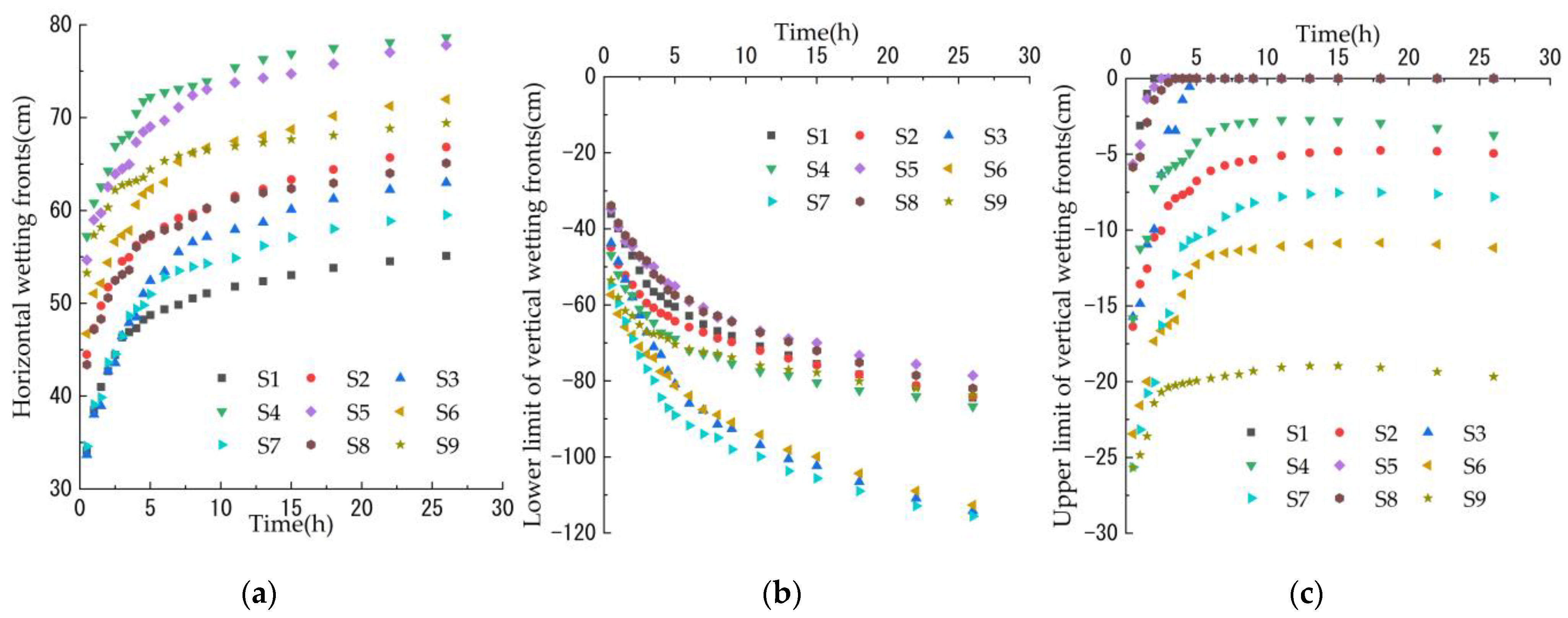
3.2. Spatial and Temporal Variation Characteristics of Wetting Fronts

Figure 5 shows the variation of the peak of wetting fronts in each direction with time during the infiltration for the nine scenarios in Table 2. With the increase in time, the peak horizontal wetting fronts gradually expanded outward (Figure 5a); the lower (Figure 5b) and upper limit (Figure 5c) of vertical wetting fronts gradually developed downward and upward, respectively. The transport rate of wetting fronts in each direction decreased with time. At the beginning of infiltration, the volume of wetted soil was smaller, the gradient soil matrix potential was higher and the transport rate of the wetting fronts was higher. Then, the size of wetted soil volume increased with time, while the gradient of matrix potential decreased, thus causing a decreasing transport rate of wetting fronts.
From Figure 5, in the scenarios of individual fruit trees with 40 L of irrigation water (Scenarios 1, 2 and 9), the wetting front depth reached about 86 cm, and the horizontal wetting front reached 55.6~69.8 cm. This can already meet the water absorption requirements of root systems of apple [37] and jujube [38] trees in arid areas and can help to save about 50% of irrigation water compared with the surge-root irrigation of individual trees [34]. This indicates that the utilization efficiency of irrigation water was significantly improved.
From the start of irrigation to the occurrence of interference infiltration, the wetted soil volume formed by each orifice outflow did not interfere with each other and can be regarded as an independent subsurface single-point source infiltration. After interference infiltration, adjacent wetted soil volume continued to infiltrate under the mutual influence. The wetted front reached a steady state 24 h after the end of irrigation. Therefore, based on the occurrence of interference infiltration, the entire infiltration period can be divided into two processes, i.e., pre-interference infiltration and post-interference infiltration. The pre-interference infiltration process indicates the process from the start of irrigation to the occurrence of interference infiltration; the post-interference infiltration process indicates the period from the occurrence of interference infiltration to the stabilization of the wetting front.

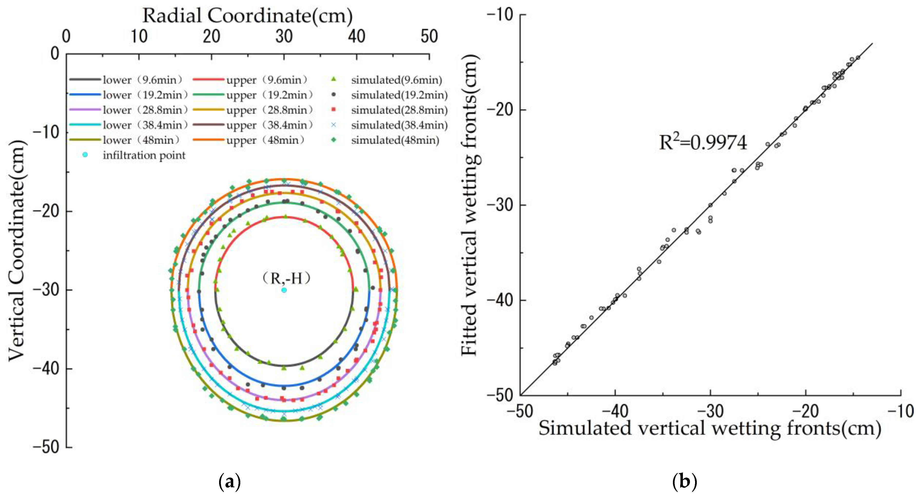
3.2.1. Pre-Interference Infiltration

The infiltration simulation results of the nine orthogonal scenarios show that interference infiltration occurred at different moments in each scenario. The statistical regression results show that the moment (ti) of interference infiltration showed a good power function relationship with the parameters in Table 2.
t i = 0.001 R 3.048 M 1.709 H 0.083 V 0.026 ( R 2 = 0.996 )
The magnitude of the absolute value of the standardized regression coefficient directly reflected the degree of influence of the influencing factors on the wetting front; the positive and negative values indicated the positive and negative correlation. The standardized regression coefficients of R, M, H and V in Equation (4) were 0.87, −0.488, 0.024 and 0.008, respectively, indicating that the influence on the moment of interference infiltration was ranked as: R > M > H > V. This is due to the fact that the spatial distance of adjacent orifices and infiltration rate are two major factors affecting the interference infiltration moment. A larger irrigation ring radius R induced a larger orifice spacing and thus a larger moment of interference infiltration. A larger orifice number M induced a smaller orifice spacing and thus a smaller moment of interference infiltration. The burial depth had a relatively small influence on the moment of interference infiltration. Due to the horizontal burial of the irrigation ring, the burial depth did not affect the adjacent orifice spacing. However, at a larger burial depth, the resistance to soil water transport was larger, the infiltration rate was smaller, and thus, the interference infiltration moment was larger. The irrigation water amount showed slight effects on the interference infiltration moment and can be ignored. Since the irrigation of each scenario was not completed when the interference infiltration occurred and the infiltration flow rate of each scenario was the same, the irrigation amount did not affect the interference infiltration moment.
In each scenario, before the interference infiltration, the wetting fronts on the vertical orifice plane showed a shape of upper and lower elliptical curves centered on the infiltration point. The vertical wetting fronts below the infiltration point were larger than the horizontal wetting fronts but smaller than the horizontal wetting front above the infiltration point. This is due to the fact that the matrix potential and gravitational potential were the main driving forces of soil water transport at the early stage of infiltration. The water was transported downward under the combined action of gravitational and matrix potentials, and only upward under the action of the matrix. Thus, the wetting front curve at a certain moment on the vertical orifice plane (xoz) can be divided into upper and lower semi-ellipse, and the long axis of the upper semi-ellipse was the short axis of the lower semi-ellipse. The distances of the peak of the wetting front relative to the infiltration point in the horizontal, vertical downward and vertical upward directions were defined as a, b and c, respectively. Then, b and a were the long axis and short axis of the lower semi-ellipse, respectively; a and c were the long axis and short axis of the upper semi-ellipse, respectively. Thus, the wetting front curve below and above the infiltration point can be expressed in elliptic equations, i.e., Equations (5) and (6), respectively:
( x R ) 2 a 2 + ( z + H ) 2 b 2 = 1 ( z H )
( x R ) 2 a 2 + ( z + H ) 2 c 2 = 1 ( z > H )
The test results of the wetting fronts of the nine scenarios at each moment before the interference infiltration were statistically regressed. It is found that the coefficients a, b and c showed a good power function relationship with the parameters R, M, H and V as well as the pre-interference infiltration time t before the interference infiltration.
{ a = 9.12 R 0.05 M 0.425 H 0.114 V 0.108 t 0.306 ( R 2 = 0.982 ) b = 6.194 R 0.028 M 0.456 H 0.132 V 0.126 t 0.339 ( R 2 = 0.989 ) c = 2.078 R 0.035 M 0.467 H 0.091 V 0.06 t 0.26 ( R 2 = 0.979 )
Substituting Equation (7) into Equations (5) and (6), then
( x R ) 2 83.176 R 0.1 M 0.85 H 0.228 V 0.216 t 0.612 + ( z + H ) 2 38.371 R 0.056 M 0.912 H 0.264 V 0.252 t 0.678 = 1 ( z H )
( x R ) 2 83.176 R 0.1 M 0.85 H 0.228 V 0.216 t 0.612 + ( z + H ) 2 145.881 R 0.07 M 0.934 H 0.182 V 0.12 t 0.52 = 1 ( z > H )
Scenario 2 was selected to verify the accuracy of Equations (8) and (9). The parameters of this scenario and the first five different moments of pre-interference infiltration (48 min) were input into Equations (8) and (9). Thus, 10 semi-elliptical curves were obtained, which were compared with the HYDRUS simulation results (Figure 6a). The 10 semi-elliptical curves were in good agreement with the simulation results. The simulated vertical wetting fronts corresponding to each radial coordinate were compared with the fitted vertical wetting fronts (Figure 6b), and the negative correlation coefficient was 0.9974. This indicates that wetting front curves of the single-point source infiltration with different parameters and at different moments can be obtained using Equations (8) and (9).

3.2.2. Post-Interference Infiltration

For sandy loam soil, during the post-interference infiltration process with a constant inflow rate, the transport distance of wetting fronts in each direction was related to the irrigation ring radius, the number of orifices, the burial depth of the irrigation ring, the irrigation water amount and the infiltration time. A large number of studies about point-source and line-source soil infiltration show that the wetted soil volume transport process can be described by the power function, with high accuracy [37,39,40]. It is assumed that the power function relationship between the transport distance of wetting fronts in each direction and the above influencing factors is
x 1 = k 1 R a 1 M b 1 H c 1 V d 1 T e 1
z 1 = k 2 R a 2 M b 2 H c 2 V d 2 T e 2
z 2 = k 3 R a 3 M b 3 H c 3 V d 3 T e 3
where the following are defined: x1 is the transport distance of the radial wetting front relative to the z-axis; z1 and z2 are the transport distances of the lower and upper vertical wetting fronts relative to the ground surface, respectively (cm); R is the irrigation ring radius (cm); M is the number of orifices on the irrigation ring; H is the burial depth of the irrigation ring (cm); V is the irrigation water amount (cm3); T is the infiltration time starting from the interference infiltration (h); k1, k2, k3, a1, a2, a3, b1, b2, b3, c1, c2, c3, d1, d2, d3, e1, e2 and e3 are empirical parameters.
The data of the wetting fronts in each direction at different moments of the nine scenarios after the interference infiltration (Figure 5) were substituted into Equations (10)–(12), and Equations (13)–(15) were obtained after logarithmic processing and multiple linear regression. Based on the regression analysis with SPSS software, it is found that the coefficients of determination (R2) of Equations (13)–(15) were 0.951, 0.961 and 0.878, respectively, with p-values less than 0.05, indicating that Equations (13)–(15) can better reflect the relationship of the spatial and temporal variation of the root emitter with its influencing factors.
x 1 = 3.42 R 0.416 M 0.054 H 0.037 V 0.112 T 0.103 ( R 2 = 0.956 )
z 1 = 4.285 R 0.24 M 0.03 H 0.427 V 0.169 T 0.2 ( R 2 = 0.962 )
z 2 = 0.035 R 0.819 M 0.204 H 3.677 V 0.873 T 0.257 ( R 2 = 0.888 )

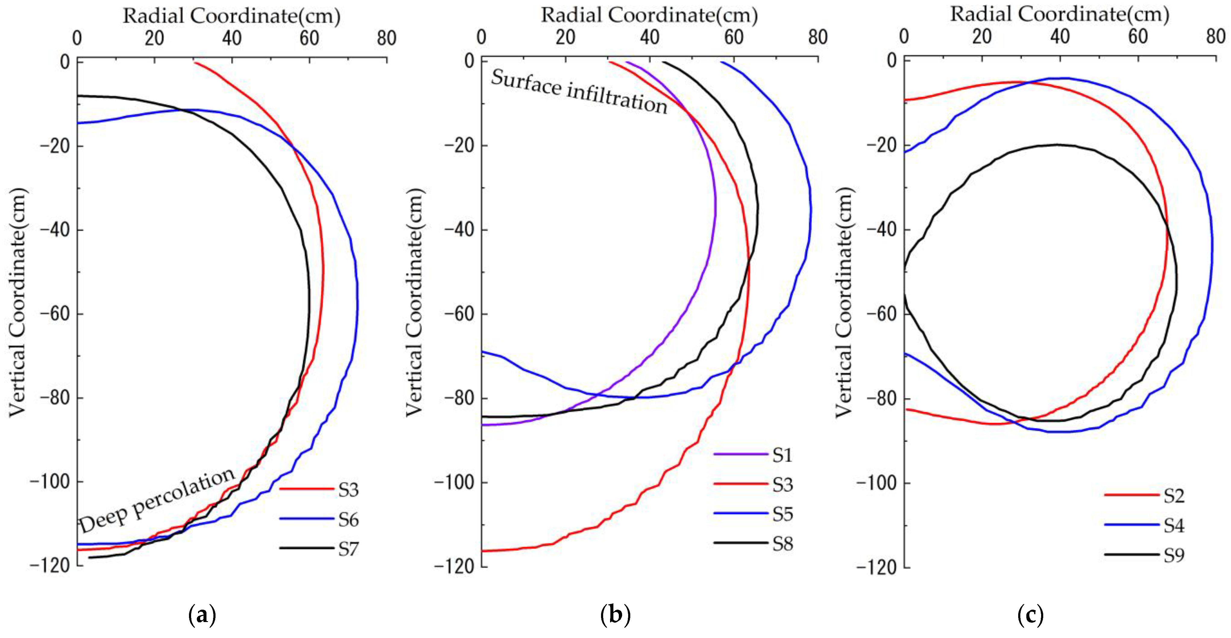
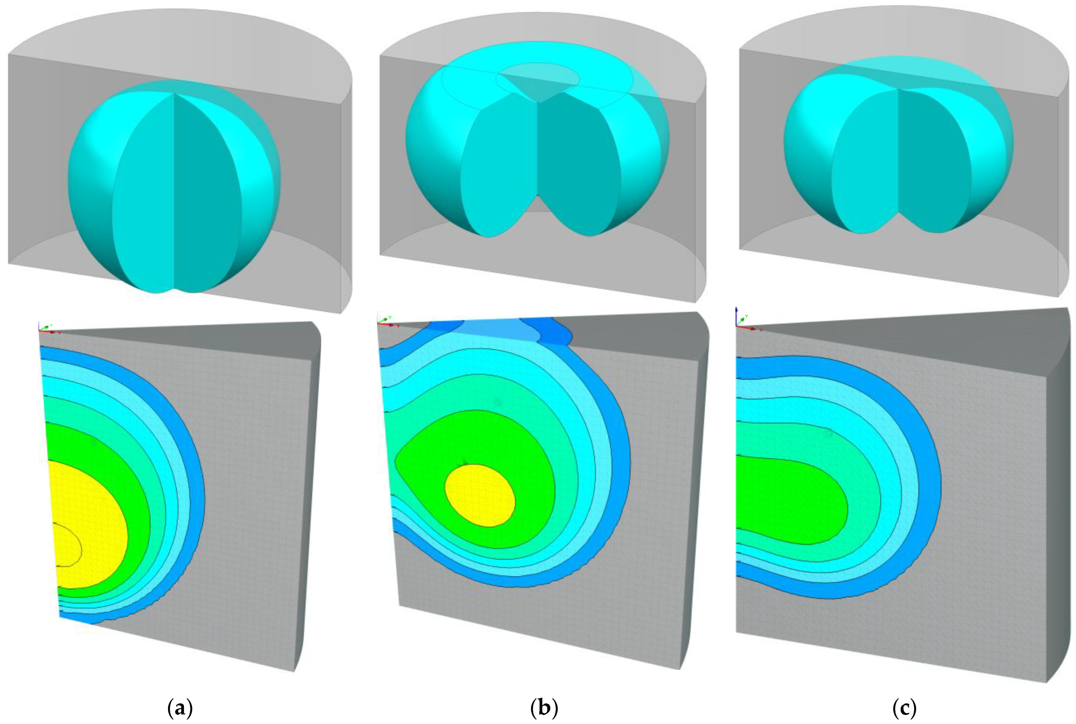
3.3. Shape of Wetted Soil Volume at Steady-State Infiltration

The peak of the wetting front only reflects the extreme value of wetted soil volume in different directions, while the wetting front curve can more intuitively reflect the morphological characteristics of wetted soil volume. The morphology of wetted soil volume after infiltration stabilization has important guiding significance for root irrigation technology. The data of the wetting front on the vertical orifice plane after infiltration stabilization of nine scenarios were plotted to obtain wetting front curves. According to the characteristics of Wetted soil volume, the nine scenarios can be divided into three categories: deep percolation scenario (Figure 7a), surface infiltration scenario (Figure 7b) and suitable infiltration scenario (Figure 7c). From Figure 7a, the lower limit of the Wetted soil volume after the stabilization of infiltration in Scenarios 3, 6 and 7 lay within 114.8–118.2 cm, which exceeded the depth of the main water-absorbing root system of the mature fruit trees. Thus, deep percolation occurred. This is due to the fact that the larger burial depth of the irrigation ring in Scenarios 6 and 7 caused their wetted soil volume to expand downward and then the deep percolation was developed. From Figure 7b, the upper limit of wetting fronts of Scenarios 1, 3, 5 and 8 rose to 0 during the infiltration, and then surface infiltration was developed. This is due to the fact that the shallow burial depth of Scenarios 1, 5 and 8 caused their wetted soil volume to expand upward as a whole, and then surface infiltration occurred. Although the burial depth of Scenario 3 was relatively moderate, the overall wetted soil volume was larger due to its excessive irrigation amount, resulting in both surface infiltration and deep percolation. Except for the above scenarios, no deep percolation and surface infiltration occurred in Scenarios 2, 4 and 9 (Figure 7c).
After stabilization of infiltration, the wetting front curve on the vertical orifice plane and the vertical intersecting plane almost overlapped. Thus, the shape of the wetted soil volume after stabilization of infiltration can be regarded as a rotating body formed by the vertical wetting front plane around the z-axis. The rotating body of the wetted soil volume of Scenario 7 (Figure 8a) with deep percolation, Scenario 5 (Figure 8b) with surface infiltration and Scenario 2 (Figure 8c) with suitable infiltration were selected. The wetted soil volume of deep percolation, surface infiltration and suitable infiltration scenarios was nearly rugby-shaped (Figure 8a), apple-shaped with a flattened top (Figure 8b) and complete apple-shaped (Figure 8c), respectively.
The results of the longitudinal wetting front regression show that the downward infiltration distance was about twice larger than the upward infiltration distance. Therefore, the recommended burial depth of the irrigation ring was slightly larger than one-third of the root depth, while burying the moistube at half the depth of the crop root zone is recommended [17]. This difference was mainly due to the gravitational potential under the conditions of root irrigation with ring-shaped emitters, While due to the slow discharge of moistube, the water movement after seepage from moistube is mainly driven by soil suction, not gravity [41], and the variability of the longitudinal distribution of the two subsurface irrigation wetted soil volumes resulted in their different suitable burial depths. The horizontal wetting front was approximately equal to the irrigation ring diameter. It is recommended that half of the horizontal range of the crop root system be selected as the radius of irrigation rings, which can enhance the utilization efficiency of irrigation water.

4. Conclusions

Fruit tree root irrigation is a highly efficient water-saving irrigation method. The ring-shaped root emitter of fruit trees forms an enclosed-shaped wetted soil volume in the root zone of fruit trees through interference infiltration of subsurface ring-shaped multiple-point sources. The multi-point source infiltration has a greater water-saving advantage than surface micro-irrigation and single-point source infiltration. In this paper, the spatial and temporal characteristics of wetted soil volume of the ring-shaped root emitter in sandy loam soil were investigated through laboratory tests and HYDRUS simulations. The following conclusions were obtained:
(1)
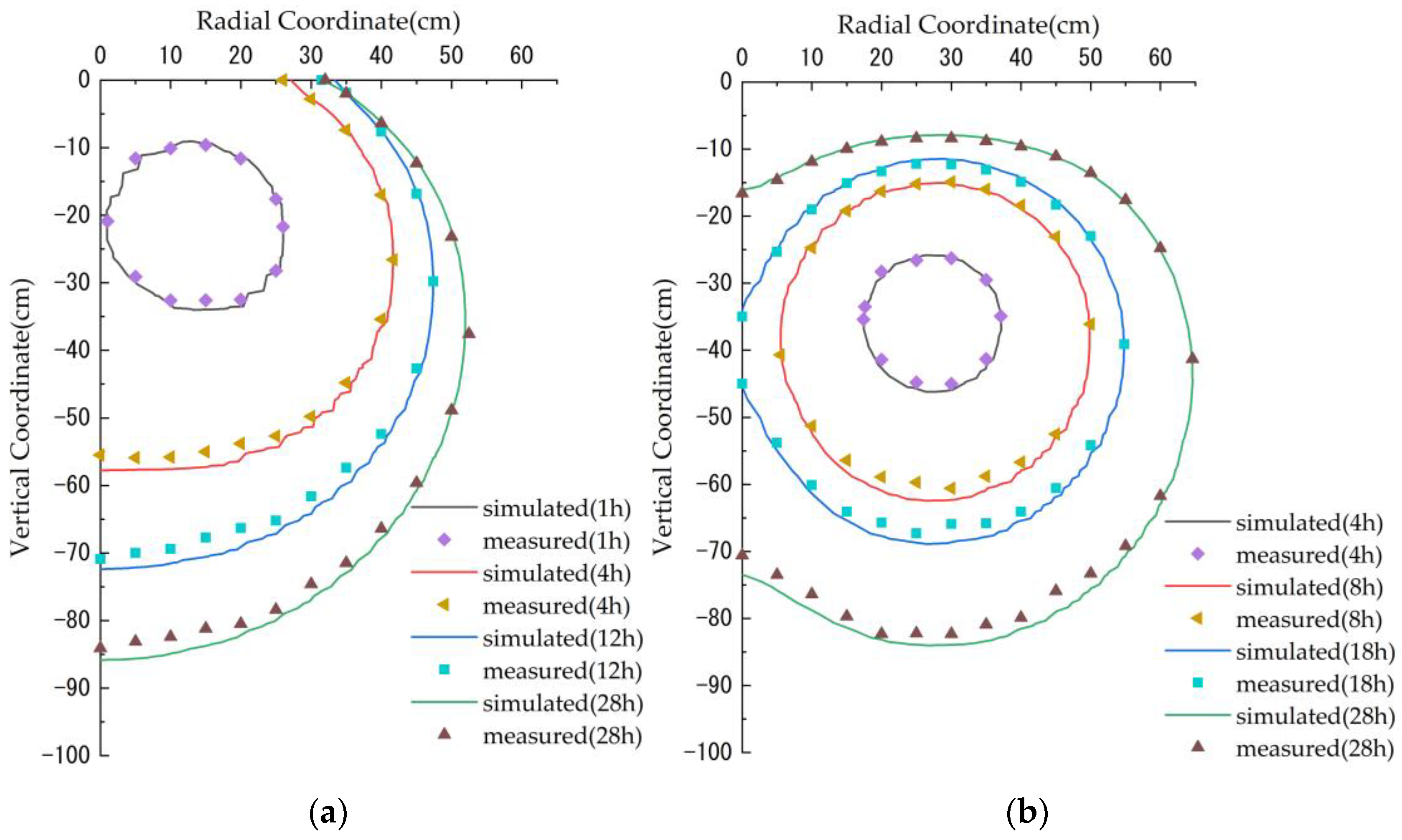
The subsurface ring-shaped multi-point source infiltration in sandy loam was simulated using HYDRUS-3D software. The simulated wetting fronts at different moments fitted well with the measured wetting front, with root mean square error less than 1.8 cm, average relative error less than 2.93% and average absolute error less than 1.5 cm. This indicates that it is feasible to use HYDRUS to simulate the multi-point source interference infiltration process.
(2)
At the early stage of infiltration, the infiltration belonged to independent subsurface single-point source infiltration before the intersection of the wetting fronts formed by the outflow of each orifice. The interference infiltration moment had a good power function relationship with the irrigation ring radius, the number of orifices and the burial depth while being independent of the irrigation water amount. The wetting fronts before interference infiltration were all in the form of a rotating ellipsoid centered on the infiltration point. The wetting fronts can be expressed by the equations of the upper and lower semi-ellipsoidal curves relative to the infiltration point, and the complex correlation coefficient of the verification results was 0.9974.
(3)
With the increase in time, the wetting front infiltrated in all directions with the infiltration point as the center, and the transport rate decreased. The power function relationship between the wetting front and the influencing factors after the interference infiltration in different directions was established, and the coefficients of determination were above 0.888.
(4)
The shape of the wetted soil volume after infiltration stabilization can be regarded as a rotating body formed by the vertical wetting front plane around the z-axis. The Wetted soil volume of deep percolation, surface infiltration and suitable infiltration scenarios was nearly rugby-shaped, apple-shaped with a flattened top and complete apple-shaped, respectively. Burying the irrigation ring at slightly deeper than one-third of the crop root zone is recommended, and half of the horizontal range of the crop root system can be selected as the irrigation ring radius.

5. Patents

The patent granted in China is related to this paper:
Author: Lin, L.; Jun, Z.; Yuan, F.S.; Hai T.Y.: A type of fruit tree root emitter. Patent No. ZL 2021 2 1009541.2, granted on 26 November 2021.

Author Contributions

Writing—original draft preparation, J.Z.; writing—review and editing, L.L.; funding acquisition, L.L. All authors have read and agreed to the published version of the manuscript.

Funding

This research was funded by “water conservancy engineering” key discipline research project of postgraduate in 2019 (Project No. SLXK-YJS-2019-03).

Data Availability Statement

All data generated or analyzed during this study are included in this article.

Conflicts of Interest

The authors declare no conflict of interest.

References

  1. Nazari, E.; Besharat, S.; Zeinalzadeh, K.; Mohammadi, A. Measurement and simulation of the water flow and root uptake in soil under subsurface drip irrigation of apple tree. Agric. Water Manag. 2021, 255, 106972. [Google Scholar] [CrossRef]
  2. Bainbridge, D.A. Buried clay pot irrigation: A little known but very efficient traditional method of irrigation. Agric. Water Manag. 2001, 48, 79–88. [Google Scholar] [CrossRef]
  3. Du, S.; Kang, S.; Li, F.; Du, T. Water use efficiency is improved by alternate partial root-zone irrigation of apple in arid northwest China. Agric. Water Manag. 2016, 179, 184–192. [Google Scholar] [CrossRef]
  4. Cook, F.; Thorburn, P.; Fitch, P.; Bristow, K. WetUp: A software tool to display approximate wetting patterns from drippers. Irrig. Sci. 2003, 22, 129–134. [Google Scholar] [CrossRef]
  5. Moncef, H.; Khemaies, Z. An analytical approach to predict the moistened bulb volume beneath a surface point source. Agric. Water Manag. 2016, 166, 123–129. [Google Scholar] [CrossRef] [Green Version]
  6. Philip, J.R. Travel Times from Buried and Surface Infiltration Point Sources. Water Resour. Res. 1984, 20, 990–994. [Google Scholar] [CrossRef]
  7. Šimůnek, J.; van Genuchten, M.T.; Šejna, M. Development and Applications of the HYDRUS and STANMOD Software Packages and Related Codes. Vadose Zone J. 2008, 7, 587–600. [Google Scholar] [CrossRef] [Green Version]
  8. Brandt, A.; Bresler, E.; Diner, N.; Ben-Asher, I.; Heller, J.; Goldberg, D. Infiltration from a Trickle Source: I. Mathematical Models. Soil Sci. Soc. Amer. Proc. 1971, 35, 675–682. [Google Scholar] [CrossRef]
  9. Malek, K.; Peters, R.T. Wetting pattern models for drip irrigation: New empirical model. J. Irrig. Drain. Eng. 2011, 137, 530–536. [Google Scholar] [CrossRef]
  10. Al-Ogaidi, A.A.; Wayayok, A.; Rowshon, M.; Abdullah, A.F. Wetting patterns estimation under drip irrigation systems using an enhanced empirical model. Agric. Water Manag. 2016, 176, 203–213. [Google Scholar] [CrossRef]
  11. Schwartzman, M.; Zur, B. Emitter spacing and geometry of wetted soil volume. J. Irrig. Drain. Eng. 1986, 112, 242–253. [Google Scholar] [CrossRef]
  12. Zhiguang, D.; Liangjun, F.; Ping, L.; Lin, C.; Yun, Z. Suitable Strategy of Water–Nitrogen Management for Surge-Root Irrigation of Jujube in China. Agron. J. 2018, 110, 1390–1401. [Google Scholar] [CrossRef]
  13. Dai, Z.; Fei, L.; Huang, D.; Zeng, J.; Chen, L.; Cai, Y. Coupling effects of irrigation and nitrogen levels on yield, water and nitrogen use efficiency of surge-root irrigated jujube in a semiarid region. Agric. Water Manag. 2019, 213, 146–154. [Google Scholar] [CrossRef]
  14. Cai, Y.; Wu, P.; Zhang, L.; Zhu, D.; Chen, J.; Wu, S.J.; Zhao, X. Simulation of soil water movement under subsurface irrigation with porous ceramic emitter. Agric. Water Manag. 2017, 192, 244–256. [Google Scholar] [CrossRef]
  15. Cai, Y.; Zhao, X.; Wu, P.; Zhang, L.; Zhu, D.; Chen, J.; Lin, L. Ceramic patch type subsurface drip irrigation line: Construction and hydraulic properties. Biosyst. Eng. 2019, 182, 29–37. [Google Scholar] [CrossRef]
  16. Dirwai, T.L.; Mabhaudhi, T.; Kanda, E.K.; Senzanje, A. Moistube irrigation technology development, adoption and future prospects: A systematic scoping review. Heliyon 2021, 7, e06213. [Google Scholar] [CrossRef]
  17. Qi, W.; Zhang, Z.; Wang, C.; Huang, M. Prediction of infiltration behaviors and evaluation of irrigation efficiency in clay loam soil under Moistube irrigation. Agric. Water Manag. 2021, 248, 106756. [Google Scholar] [CrossRef]
  18. Rodríguez-Sinobas, L.; Zubelzu, S.; Martín-Sotoca, J.J.; Tarquis, A.M. Multiscaling analysis of Soil Water Content during irrigation events. Comparison between surface and subsurface drip irrigation. Geoderma 2021, 382, 114777. [Google Scholar] [CrossRef]
  19. Mattar, M.A.; El-Abedin, T.; Al-Ghobari, H.M.; Alazba, A.A.; Elansary, H.O. Effects of different surface and subsurface drip irrigation levels on growth traits, tuber yield, and irrigation water use efficiency of potato crop. Irrig. Sci. 2021, 39, 517–533. [Google Scholar] [CrossRef]
  20. Wei, W.Y.; Xiao, Y.M.; Li, J.; Parkes, M. Simulation of point source wetting pattern of subsurface drip irrigation. Irrig. Sci. 2011, 29, 331–339. [Google Scholar] [CrossRef]
  21. Singh, D.K.; Rajput, T.; Sikarwar, H.S.; Sahoo, R.N.; Ahmad, T. Simulation of soil wetting pattern with subsurface drip irrigation from line source. Agric. Water Manag. 2006, 83, 130–134. [Google Scholar] [CrossRef]
  22. Appels, W.M.; Karimi, R. Analysis of soil wetting patterns in subsurface drip irrigation systems—Indoor alfalfa experiments. Agric. Water Manag. 2021, 250, 106832. [Google Scholar] [CrossRef]
  23. Siyal, A.A.; Skaggs, T.H. Measured and simulated soil wetting patterns under porous clay pipe sub-surface irrigation. Agric. Water Manag. 2009, 96, 893–904. [Google Scholar] [CrossRef]
  24. Monjezi, M.S.; Ebrahimian, H.; Liaghat, A.; Moradi, M.A. Soil-wetting front in surface and subsurface drip irrigation. Proc. Inst. Civ. Eng. Water Manag. 2013, 166, 272–284. [Google Scholar] [CrossRef]
  25. Mei, X.N.; Shen, Z.Z.; Ren, J.; Wang, Z.H. Effects of Dripper Discharge and Irrigation Amount on Soil-Water Dynamics under Subsurface Drip Irrigation. Adv. Mater. Res. 2011, 347–353, 2400–2403. [Google Scholar] [CrossRef]
  26. Zare, E.; Arshad, M.; Zhao, D.; Nachimuthu, G.; Triantafilis, J. Two-dimensional time-lapse imaging of soil wetting and drying cycle using EM38 data across a flood irrigation cotton field. Agric. Water Manag. 2020, 241, 106383. [Google Scholar] [CrossRef]
  27. Mohammed, A.K.; Abed, B.S. Water Distribution and Interference of Wetting Front in Stratified Soil Under a Continues and an Intermittent Subsurface Drip Irrigation. J. Green Eng. 2020, 10, 268–286. [Google Scholar]
  28. Assouline, S.; Cohen, S.; Meerbach, D.; Harodi, T.; Rosner, M. Microdrip irrigation of field crops: Effect on yield, water uptake, and drainage in sweet corn. Soil Sci. Soc. Am. J. 2002, 66, 228–234. [Google Scholar] [CrossRef]
  29. Badr, A.E.; Abuarab, M.E. Soil moisture distribution patterns under surface and subsurface drip irrigation systems in sandy soil using neutron scattering technique. Irrig. Sci. 2013, 31, 317–332. [Google Scholar] [CrossRef]
  30. Bozkurt, S.; Yazar, A.; Mansuroğlu, G.S. Effects of different drip irrigation levels on yield and some agronomic characteristics of raised bed planted corn. Afr. J. Agric. Res. 2011, 6, 5291–5300. [Google Scholar]
  31. Lamm, F.R.; Trooien, T.P. Dripline Depth Effects on Corn Production when Crop Establishment is Nonlimiting. Appl. Eng. Agric. 2005, 21, 835–840. [Google Scholar] [CrossRef] [Green Version]
  32. Fan, Y. Roots Spatial Distribution Characteristics of 9T337 Dwarfing Self-Rooted Rootstock Apple Trees from Different Ages. Master’s Thesis, Northwest Agriculture and Forestry University of Science and Technology, Xianyang, China, 2019. [Google Scholar]
  33. Zhongjie, L.; Liangjun, F.; Kun, H.; Teng, L.; Nanshu, C.; Quanju, Z.; Deliang, H. Effects of arrangement of surge-root irrigation emitters on growth, yield and water use efficiency of apple trees. J. Drain. Irrig. Mach. Eng. 2020, 38, 7. [Google Scholar]
  34. Zhang, L.J.; Wang, Y.K.; Xin, X.G.; Hong-Yan, L.I. Appropriate surge spring root irrigation layout and irrigation norm of jujube on mountain land. J. Northwest A F Univ. 2010, 38, 211–217. [Google Scholar] [CrossRef]
  35. Zhenjia, H.E. Effects of Irrigation Quota under Bubbled-root Irrigation on Soil Water Dynamic Changes and Water Use Efficiency of Jujube. J. Irrig. Drain. 2018, 37, 45–49. [Google Scholar]
  36. Saefuddin, R.; Saito, H.; Šimůnek, J. Experimental and numerical evaluation of a ring-shaped emitter for subsurface irrigation. Agric. Water Manag. 2018, 211, 111–122. [Google Scholar] [CrossRef]
  37. Fan, Y.; Shao, X.; Gong, J.; Wang, Y. An Empirical Model for Estimating Soil Wetting Pattern Dimensions during Film Hole Irrigation. Arch. Agron. Soil Sci. 2019, 66, 1765–1779. [Google Scholar] [CrossRef]
  38. Sun, S.; An, Q.; Yang, P.; Lu, X.; Gu, K. Effect of Irrigation Depth on Root Distribution and Water Use Efficiency of Jujube under Indirect Subsurface Drip Irrigation. Trans. Chin. Soc. Agric. Mach. 2016, 47, 81–90. [Google Scholar]
  39. Al-Ogaidi, A.; Wayayok, A.; Kamal, M.R. (Eds.) Modelling Soil Wetting Patterns under Drip Irrigation Using Hydrus-3D and Comparison with Empirical Models. In Proceedings of the Global Conference on Engineering and Technology (GCOET), Kuala Lumpur, Malaysia, 1–2 June 2016. [Google Scholar]
  40. Nagli, B.; Kechavarzi, C.; Coulon, F.; Pintar, M. Numerical investigation of the influence of texture, surface drip emitter discharge rate and initial soil moisture condition on wetting pattern size. Irrig. Sci. 2014, 32, 421–436. [Google Scholar] [CrossRef]
  41. Sun, Q.; Wang, Y.; Geng, C.; Hui, Y.; Du, T. Water use efficiency was improved at leaf and yield levels of tomato plants by continuous irrigation using semipermeable membrane. Agric. Water Manag. 2018, 203, 430–437. [Google Scholar] [CrossRef]
Figure 1. Working principle of the root emitter.
Sustainability 14 06712 g001
Figure 2. Schematic diagram of root emitter infiltration test. (a) Test apparatus; (b) Cross-section of the irrigation ring.
Sustainability 14 06712 g002
Figure 3. HYDRUS calculation area. (a) Mesh of calculation area; (b) Mesh of ponding area.
Sustainability 14 06712 g003
Figure 4. Comparison of simulated and measured values. (a) Scenario 1; (b) Scenario 4.
Sustainability 14 06712 g004
Figure 5. Changes in the peak of wetting fronts in each direction with time. (a) horizontal; (b) lower limit of vertical; (c) upper limit of vertical.
Sustainability 14 06712 g005
Figure 6. Comparison of the simulated and fitted pre-interference infiltration wetting fronts (Scenario 2). (a) Semi-elliptical curves and simulation results; (b) Simulated and fitted values.
Sustainability 14 06712 g006
Figure 7. Wetting front curves on the vertical orifice plane after stabilization of infiltration. (a) deep percolation; (b) surface infiltration; (c) suitable infiltration.
Sustainability 14 06712 g007
Figure 8. Three-dimensional view of the shape of the wetted soil volume after stabilization by infiltration. (a) Scenario 7; (b) Scenario 5; (c) Scenario 2.
Sustainability 14 06712 g008
Table 1. Orthogonal design scenario.
ScenarioR (cm)MH (cm)V (cm3)
12042040,000
23063040,000
32083080,000
44043060,000
54062080,000
63044080,000
72064060,000
83082060,000
94084040,000
Table 2. Soil water transport parameters.
θr
(cm3·cm−3)
θs
(cm3·cm−3)
α
(cm−1)
nKs
(cm·h−1)
I
0.03480.37420.01591.47212.20890.5
Table 3. Differences between measured and simulated values.
DifferencesS1S4
1 h4 h12 h284 h8 h12 h28 h
RMSE (cm)0.721.471.801.530.901.241.151.47
RE (%)2.772.922.932.362.142.222.742.52
MAE (cm)0.611.211.501.240.790.960.961.11
S1 represents Scenario 1 and S4 represents Scenario 4.
Publisher’s Note: MDPI stays neutral with regard to jurisdictional claims in published maps and institutional affiliations.

