Investigation of Whether People Are Willing to Pay a Premium for Living in Food Swamps: A Study of Edmonton, Canada

Abstract

Extensive studies have examined how unfavorable food environments, especially food swamps (neighborhoods with oversaturated unhealthy food sources), influence people’s dietary behaviors and health. Although excess fast-food consumption may have an adverse effect on health, it also benefits consumers due to its convenience, time saving, and affordability. Therefore, people’s preference for an unhealthy food environment is not necessarily negative. Understanding how people value or disvalue unhealthy food environments is a prerequisite for developing effective policies to promote good diet habits and improve public health. Thus, this study adopts spatial hedonic pricing models to estimate people’s willingness to pay to live in food swamps. The results show that people are willing to pay a premium to live in food swamps when taking low income and low healthy-to-unhealthy food ratios into consideration. On average, a household is willing to pay a premium of C$12,309 to reside in a food swamp neighborhood. Potential reasons for the positive willingness to pay among low-income communities and households with relatively limited access to healthy food may include the unaffordability of healthy diets, preference for better tastes, and time saved in fast-food consumption. These findings can help policymakers evaluate the effectiveness of relevant policies and develop targeted strategies to improve the local food environment.

1. Introduction

The rising prevalence of obesity has become one of the leading global public health concerns [1,2,3]. According to recent WHO estimations [3], over 1.9 billion adults and over 340 million children and adolescents were overweight or obese worldwide in 2016. Overweight and obesity have been major risk factors for many serious health issues, such as type 2 diabetes, hypertension, coronary heart disease, and other chronic diseases [4,5].

Many studies have shown that healthy eating is important for health and reduces the risk of obesity and other related chronic diseases [6,7]. Furthermore, food environments have significant impacts on people’s diet behaviors and food choices [2,8,9,10,11]. Specifically, residents with better access to supermarkets tend to consume more healthy food and are less likely to be obese [2,9,11]. In contrast, living in neighborhoods with abundant access to unhealthy food outlets, residents are likely to consume more fast foods and have a greater risk of obesity [2,12,13,14].

Given the significant influences of food environments on people’s dietary behaviors and health, one prevailing line of research has focused on identifying specific food environments that require policy attention, such as food deserts and food swamps. Roughly speaking, food deserts are neighborhoods that have limited access to nutritious and fresh food [15,16], and food swamps are neighborhoods with excessive access to unhealthy food sources [17,18,19,20]. Compared to food deserts, recent studies suggest that food swamps are more prevalent and have more substantial negative impacts on people’s diet habits and food choices, and suggest that policymakers should pay more attention to food swamps [17,18,19].

At the same time, some researchers argue that only focusing on improving the built environment will not work because this ignores the actual desires and preferences of people living in an unhealthy food environment [21,22]. For example, Alkon et al. (2013) [21] found that low-income residents’ main obstacle to obtaining healthy food is insufficient income, rather than lack of access to healthy food sources or lack of knowledge. So, low-income households may prefer to live in communities with convenient access to fast foods, given the financial constraints. Policies such as eliminating unhealthy food stores from these communities to improve the eating environment may not work and even increase the cost of living of the poor.

In addition to health and affordability issues, other vital factors that may affect people’s preference for unhealthy food environments include convenience/time saving and the taste of fast food. Therefore, an unhealthy food environment brings both costs (e.g., health effects) and benefits (e.g., time saving). Assuming that people are willing to pay a premium for benefits and require compensation for costs, the final willingness to pay (WTP) for living in such a neighborhood/environment will depend on the relative importance of these factors. It is also predictable that the WTP of the rich and the poor will be different because the relative benefits and costs of the two groups are different.

Understanding how people value or disvalue unhealthy food environments can provide insight for developing effective policies to promote good diet habits and improve public health. After all, residents can vote with their feet. If the change in the physical environment is inconsistent with people’s preferences, they may relocate to other places. As a result, the policy of environmental change may not produce the desired effect.

Thus, the main objective of this research is to investigate people’s WTP for living in unhealthy food environments. To attain our primary objective, we adopt spatial hedonic pricing models (HPM) to examine the impact of food swamps on housing prices and estimate the corresponding WTP through an empirical analysis in Edmonton, Canada. We contribute to the food environment literature as the first study to estimate people’s WTP for residing in food swamps using a hedonic method, although a few previous studies have added proximity to superstores as control variables to explore the determinants of property values in their HPM specifications. For instance, Tyvimaa et al. (2015) [23] and Heyman and Sommervoll (2019) [24] find that housing prices increase when the distances to supermarkets rise in Helsinki and Oslo, Norway, respectively. However, to our knowledge, no research has used the HPM to estimate the value of unhealthy food environments. Our findings will add value to the literature on the attitudes and preferences of people living in different food environments [21,22]. From a policy implication perspective, our results can provide critical information for designing more efficient strategies to promote healthy eating.

We also contribute to the literature by investigating and comparing three different definitions of food swamps. The concept of food swamps was first introduced by Rose et al. (2009) [20]; however, there is no uniform definition of a food swamp. Some researchers define food swamps as communities where unhealthy food choices inundate healthy food options [17,19]. Others also include the income parameter as a criterion when defining food swamps, since unhealthy food stores are found located disproportionately in low-income neighborhoods [20]. Overall, there are three measures adopted to define food swamps in the existing literature: (1) neighborhoods with high availability of unhealthy food outlets [17,18,19], (2) neighborhoods with low availability of healthy food and high coverage of unhealthy food (often measured as the healthy food ratio, i.e., healthy food outlets divided by total food outlets) [17,19], and (3) low-income neighborhoods with low availability of healthy food and high coverage of unhealthy food [20]. All three definitions are important and provide useful information. Therefore, in our empirical study, we adopt all three definitions and compare the results. By doing so, we can relate our findings to the existing literature using relevant definitions.

The remainder of the paper consists of the following sections. Section 2 provides a brief overview of the HPM and discusses spatial HPMs that can be used to solve the spatial autocorrelation problem. It also presents a way to estimate marginal effects in spatial HPMs. Section 3 describes the study area and data, and defines variables. Section 4 presents results, and Section 5 discusses the implications. Finally, conclusions and recommendations for future research are outlined in Section 6.

2. Methods

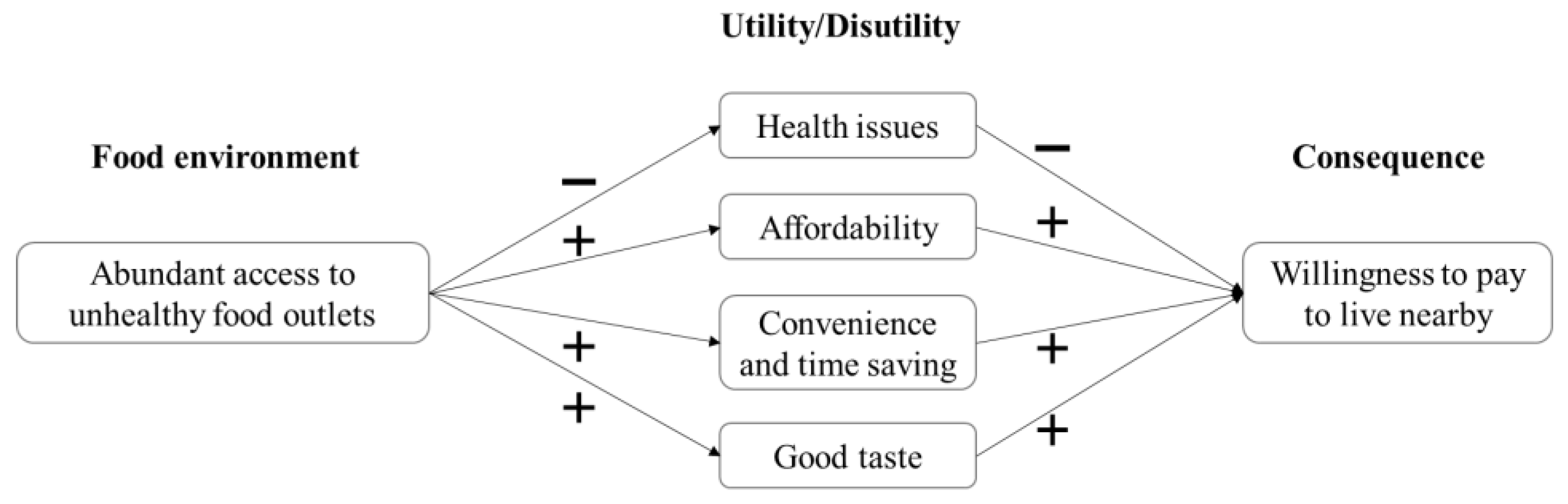
2.1. Conceptual Framework

The hedonic pricing method provides a basis for explaining housing prices as a function of the levels of characteristics embedded in each house, including the environmental quality associated with the housing unit’s location. The HPM is widely used to estimate the value of non-market goods, especially environmental amenities/disamenities (such as open space and air quality) that are not directly traded in the market [25,26,27,28]. Like environmental amenities, the food environment also represents a built environment, influencing households’ willingness to pay for properties and further affecting the demand and prices of the real estate market.

The main reason why people respond to changes in the food environment is that such changes alter (enhance or decrease) the utility of the residents. We conjecture that the main benefits and costs (which are directly related to house buyers’ utility) associated with residing in an unhealthy food environment can be grouped into four categories: potential negative influences on health (through affecting consumers’ dietary behavior), value from relatively cheap prices, benefits from convenience and time saving, and good tastes [13,17,29,30]. Each of these factors could improve or lower residents’ quality of life, which is capitalized in housing prices. Figure 1 illustrates the conceptual framework that links residing in a food swamp with people’s potential WTP through the main benefits and costs brought by the unhealthy environment. According to this framework, we propose that people’s WTP to reside in a food swamp neighborhood will depend on the relative importance of each factor. In addition, we hypothesize that the WTP of the rich and the poor will be different because the benefits and costs of the two groups are different.

2.2. Hedonic Pricing Model

An HPM is mainly composed of three types of attributes, including structural variables, locational attributes, and neighborhood characteristics [27,28,31,32]. Locational attributes (for example, distances to employment centers and parks) have been commonly added to HPMs because these sites bring value to people living near these locations [27,28,32,33]. Neighborhood socioeconomic characteristics are also closely associated with housing prices, since these characteristics often represent a bundle of local public services and amenities [31,33,34,35]. Given that our main objective is to examine the impacts of food swamps on housing prices, we include the food swamp variable into the general HPM. In sum, our HPM could be expressed in the following matrix form:

$$P=\alpha {\iota }_n+X\beta +\epsilon ,\epsilon ~N\left(0,{\sigma }^2{I}_n\right)$$

(1)

where P represents an $n\times 1$ vector of the housing prices, ${\iota }_n$ is an $n\times 1$ vector of ones associated with the constant term parameter $\alpha$. $X$ denotes an $n\times k$ matrix representing all explanatory variables, including houses’ unhealthy food environment, structural variables, locational attributes, neighborhood socioeconomic characteristics, and control variables. Specifically, structural variables contain information such as living area, lot size, house age, number of bedrooms and bathrooms, and house conditions. Locational attributes measure accessibility to Downtown, University of Alberta, rivers, hospitals, and parks. Neighborhood socioeconomic characteristics mainly include neighborhood-level census data. $\beta$ is a $k\times 1$ vector that represents the parameters of explanatory variables. $\epsilon$ is an $n\times 1$ vector of independent and identically distributed error terms.

Generally, to decide the suitable functional form of the HPM, researchers choose the functional form according to certain goodness of fit criteria [27,36]. This study estimates four functional forms of the HPM, including linear, log–log, log–linear, and semi-log forms. The log–log form generates the lowest AIC and BIC values and, therefore, is selected for further empirical analysis.

2.3. Spatial Hedonic Pricing Model

Since the attributes of properties are inherently spatially dependent (e.g., high and low property values tend to cluster together in certain neighborhoods), estimation of the HPM in Equation (1) is likely to be biased if we ignore the spatial autocorrelation. To deal with the spatial dependence issue, we employ three spatial regression models following prior studies [37,38,39]. Final model selection will depend on specific tests and model selection criteria. First, we consider the spatial lag (SAR) model, which allows for direct spatial interactions in the dependent variable:

$$P=\alpha {\iota }_n+\rho WP+X\beta +\epsilon ,\epsilon ~N\left(0,{\sigma }^2{I}_n\right)$$

(2)

where W is an n × n spatial weights matrix, the term WP represents the spatially weighted neighborhood housing prices, and ρ is a spatial autoregressive parameter for the term WP. Then, we consider the spatial error model (SEM), which can be expressed in matrix form as:

$$P=\alpha {\iota }_n+X\beta +u,u=\lambda Wu+\epsilon ,\epsilon ~N\left(0,{\sigma }^2{I}_n\right)$$

(3)

where the term Wu represents the weighted average of the disturbances, and λ is the spatial autocorrelation coefficient for the endogenous variable Wu. Finally, we consider the spatial autoregressive confused (SAC) model, which combines the SAR and SEM models. The SAC model can be expressed as follows:

$$P=\alpha {\iota }_n+\rho WP+X\beta +u,u=\lambda Wu+\epsilon ,\epsilon ~N\left(0,{\sigma }^2{I}_n\right)$$

(4)

In the SAC model, when $\rho =0$, the model becomes SEM, and when $\lambda =0$, it becomes SAR. If both parameters ($\rho ,\lambda$) are zero, then the model becomes the non-spatial standard linear regression model. We conduct the following tests to find the most suitable model to describe our data. First, we conduct a series of Moran’s I tests, Lagrange multiplier (LM) tests, and robust LM tests to check the existence of spatial effects. Then, a likelihood ratio (LR) test is used to test whether the SAC model can be simplified to a SAR or an SEM.

Regarding the weights matrix, we consider the k-nearest neighbor criterion and the contiguity-based queen criterion. For the former, we try k = 5, 10, and 20 to check the sensitivity of the results to neighbor specifications. For the latter, we first create Thiessen polygons for each house location and then choose the queen criterion to define neighbors.

2.4. Estimation of Marginal Effects

The coefficients for the non-spatial linear model and SEM can be interpreted directly as the marginal effects, which are the partial derivatives of $P_i$ with respect to $x_{ir}$ for any explanatory variable r. However, for models that contain spatial lagged dependent variable $WY$ (e.g., SAR and SAC models), the estimated marginal effects for the explanatory variables are more complicated, because the change of an explanatory variable for a given observation will affect the dependent variable in the same location directly and affect the dependent variable in all other locations indirectly. To illustrate the direct and indirect impacts in SAR and SAC models, we take a look at the marginal effects matrix $M_r\left(W\right)$ for a specific exogenous variable x_r:

$$M_r\left(W\right)=\left[\begin{array}{ccc}\frac{\partial P_1}{\partial x_{1r}}& \cdots & \frac{\partial P_1}{\partial x_{nr}}\\ ⋮& \ddots & ⋮\\ \frac{\partial P_n}{\partial x_{1r}}& \cdots & \frac{\partial P_n}{\partial x_{nr}}\end{array}\right]={(I_n-\rho W)}^{-1}\left[\begin{array}{ccc}{\beta }_r& \cdots & 0\\ ⋮& \ddots & ⋮\\ 0& \cdots & {\beta }_r\end{array}\right]={(I_n-\rho W)}^{-1}{\beta }_r$$

(5)

In Equation. (5), element $\partial P_i/\partial x_{ir}$ on the diagonal of $M_r\left(\mathrm{W}\right)$ measures the direct effect on the dependent variable P_i from a change in x_ir, and the off-diagonal element $\partial P_j/\partial x_{ir}$ of $M_r\left(\mathrm{W}\right)$ measures the indirect effect on the dependent variable P_j from a change in x_ir. LeSage and Pace (2009) [40] suggest using the average direct, the average indirect, and the average total effects to summarize the marginal effects. Specifically, the average direct effect (ADE) is the average of the diagonal terms in $M_r\left(W\right)$. The average indirect effect (AIE) is the average of the column sums of the off-diagonal elements in $M_r\left(W\right)$. The average total effect (ATE) is the summation of ADE and AIE, which is obtained by averaging all the column sums of $M_r\left(W\right)$. Furthermore, we estimate households’ marginal WTP for residing in food swamps based on the estimated marginal effects from the spatial HPMs [41]. Given the log-log form of a SAR/SAC model, the total, direct, and indirect marginal WTP for dummy variables (e.g., whether living in food swamp neighborhoods) can be expressed as:

$$\begin{array}{l}Direct WT{P}_{dummy}=\left[exp(ADE)-1\right]\stackrel{-}{P}\\ Indirect WT{P}_{dummy}=\left[exp(AIE)-1\right]\stackrel{-}{P}\\ Total WT{P}_{dummy}=\left[exp(ATE)-1\right]\stackrel{-}{P}\end{array}$$

(6)

where $\overline{P}$ represents the average value of properties in Edmonton.

3. Study Area and Data

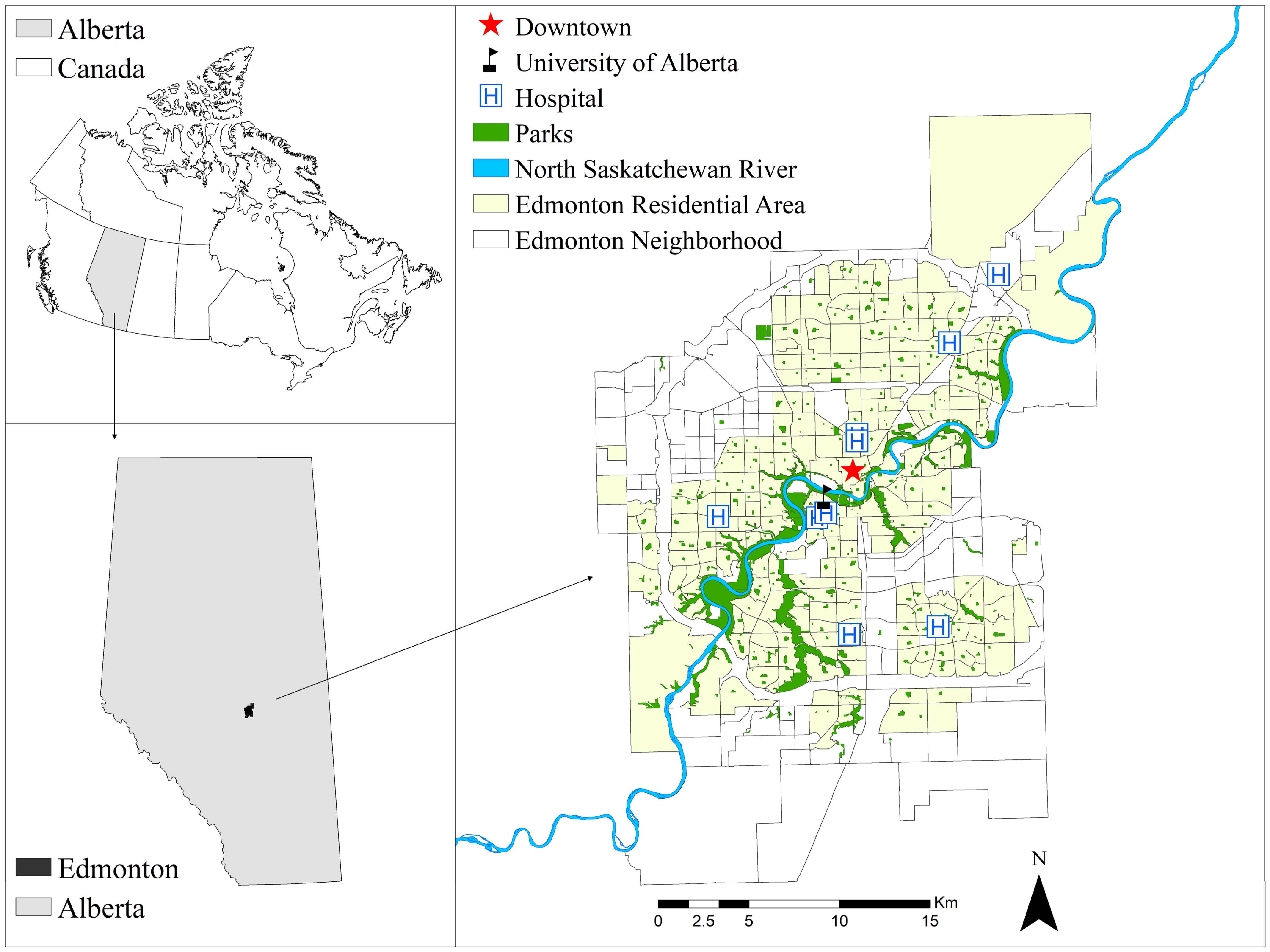
3.1. Study Area

This study is conducted in Edmonton, Alberta, Canada (see Figure 2). Edmonton is Alberta’s capital city and major economic center, with a population of 972,223 in 2019 [42]. According to a report investigated in Alberta [43], 24.1% of adults aged over 18 in Edmonton were classified as obese in 2014, higher than the national average of 20.2%. The municipal government has been making great efforts to improve residents’ eating behavior by various strategies, including creating a healthier food environment. The city’s Food and Urban Agriculture Strategy, Fresh, was launched in 2012 to make Edmonton a better place to live and work [44]. One of Fresh’s main goals is to construct a healthier and more food-secure community by increasing accessibility to enough nutritious food and encouraging families and communities to grow, preserve and purchase local food [44].

Undoubtedly, Fresh contributes to the development of a healthier and more nutritious food environment in Edmonton. Under this initiative, many strategies and programs promote healthy eating (for example, increasing the intake of healthy foods and reducing the consumption of unhealthy foods) and emphasize changing perspectives to have better lifelong eating habits. Our research on people’s preferences for unhealthy foods should provide helpful information to help Fresh develop tailor-made strategies to construct a healthier food environment and promote healthy eating.

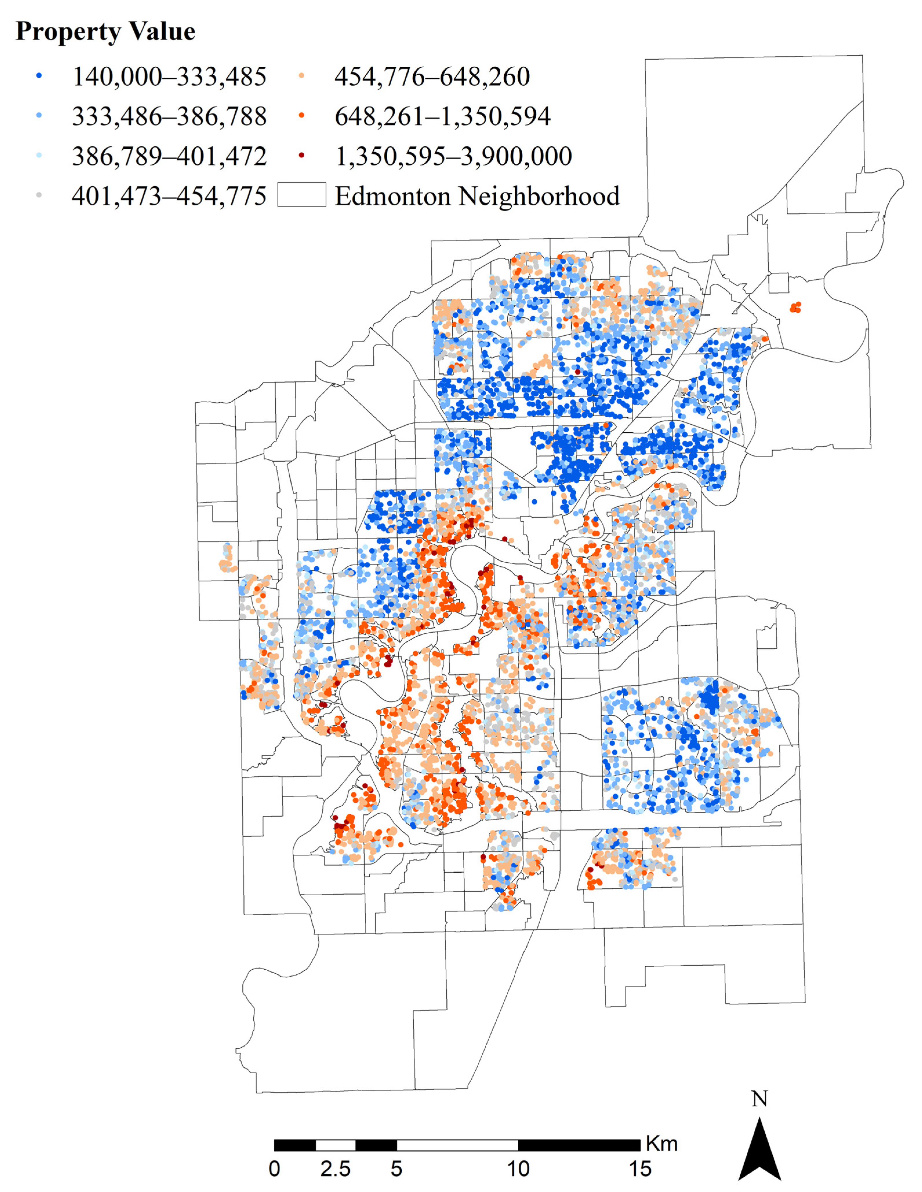
3.2. Housing Pricing Data

Mainly, two types of housing price data have been used in the HPM literature. One is the assessment data usually provided by the local government, and the other is the arm’s-length transaction data provided by private companies [45]. Compared to the transaction data, the assessment data could provide more complete housing price data. However, the assessment data may lack essential information on the structural characteristics. Furthermore, the values may not sufficiently represent the market values due to inappropriate assessment methods [45]. Transaction data are usually the recommended ones for the HPM analyses [46] (p. 317).

This study collects transaction data on single-family residential properties throughout 2015–2017 from the RPS Real Property Solutions. A total of 8241 sales transaction records are collected after excluding missing or mistyped values in the structural variables. Using the Alberta Consumer Price Index (CPI) provided by Statistics Canada (2017) [47], sales transaction prices are adjusted to 2016 Edmonton housing market values. The average sale price for the properties in our sample is 460,794.40 CAD in 2016 dollars. These transaction data also comprise detailed information about house structure characteristics and house locations. The distribution of property values in Edmonton is presented in Figure 3. It can be seen that the property values exhibit obvious spatial autocorrelation. Relatively high-priced houses are located next to each other, mainly in the southwest of the city, while relatively low-priced houses are clustered in the north and southeast of the city.

3.3. Food Outlets Data and Identifying Food Swamps

As discussed in the introduction, we investigate food swamps with three different definitions. Definition 1 considers only the high availability of unhealthy food outlets. We set the top quantile of the number of service areas as an indicator of the high availability of unhealthy food outlets. Definition 2 adds the condition of a low level of healthy food ratio (by selecting below the median level of healthy-to-unhealthy food ratio) to define food swamps. Based on Definition 2, Definition 3 further incorporates the criterion of low income (choosing above the city median level of low-income rate) to define food swamps.

To identify food swamps, we first collected the locations of unhealthy food stores (fast food restaurants and convenience stores) and healthy food stores (supermarkets and grocery stores) from the City of Edmonton business licenses database (2018) [48]. Fast food restaurants are defined as quick service food outlets that offer consistent, popular, high-calorie, and expedited food such as sandwiches, hamburgers, fried chicken, and pizza [13,49]. Because of the standardized menu and pre-cooked foods, customers only need to spend minimal time obtaining product information and receiving their meals [13]. Convenience stores are also considered unhealthy food outlets because they predominantly stock non-perishable items, including snacks, sweets, and junk foods [50,51]. Supermarkets and grocery stores are healthy stores that sell and consistently stock a wide range of products, including fresh produce, dairy items, and meat products [51].

Labeling franchised fast-food restaurants and convenience stores as unhealthy food stores, and supermarket chains and local grocery stores as healthy food stores is a bit strong. However, in practice, it is difficult to completely distinguish between healthy and unhealthy food stores. In addition, relevant data are usually not available. Therefore, in the food environment literature (see, for example, [16,17,52]), it is a common practice to label fast-food restaurants and convenience stores as unhealthy food stores, and treat supermarket chains and local grocery stores as healthy food retailers. The main criterion adopted by the literature to distinguish healthy/unhealthy food stores is whether the store has the potential to provide a wide range of healthy and fresh foods.

After we cross-validated all the food stores’ information by checking their official website and Google Map locations, a total of 822 fast food restaurants, 232 convenience stores, 91 supermarkets, and 87 grocery stores were identified in Edmonton. Then, we followed recent studies in Edmonton [53,54] and chose 1000 meters as the threshold to create a service area around each unhealthy food outlet. Finally, we counted the total number of service areas within each neighborhood and used the number of service areas as the baseline criterion to identify food swamps.

3.4. Locational Attributes Data

We collected the locations of River, Downtown, University, hospitals, and parks from various sources. The North Saskatchewan River is a majestic river that flows through Edmonton (See Figure 2). The river provides Edmontonians with various recreation activities, including canoeing, kayaking, jet-skiing, and fishing [55]. We obtained the North Saskatchewan River shapefile from the Alberta Government (2018) [56]. Downtown Edmonton is the central business district of Edmonton and is home to more than 200 eateries and hundreds of shops [57]. The University of Alberta is one of Canada’s top universities and is Alberta’s 4th largest employer, hiring almost 15,000 employees [58]. We extracted the locations of Downtown, University of Alberta, and hospitals from the City of Edmonton Open Data Catalogue (2016) [59]. To generate locational attributes for each property, we calculated road network distances to the North Saskatchewan River, the centroid of Downtown, the University of Alberta, and the nearest hospital.

Along the North Saskatchewan Riverbank is a chain of city parks collectively known as the North Saskatchewan River Valley Parks System. This Parks System is Canada’s largest stretch of urban parks and comprises over 20 major parks. In addition to this Parks System, there are over 500 neighborhood and city parks across the city. We obtained all the park location information from the City of Edmonton Open Data Catalogue (2016) [59]. To measure access to parks, we first created a 200-m buffer area around each property and then calculated the area in square meters of parks within each buffer.

3.5. Neighborhood Socioeconomic Data

Neighborhood socioeconomic data for 2016 are extracted from the City of Edmonton Open Data Catalogue (2018) [60]. After excluding industrial neighborhoods, we recognized 247 residential neighborhoods and focused on them in empirical investigation. Following previous studies [31,35,61], we include neighborhood-level population density (Population density), the ratio of children aged under 14 (Children), the ratio of the senior population aged over 60 (Senior), the ratio of residents who have a postsecondary certificate (High education), and the ratio of unemployed residents (Unemployment). Except for the above explanatory variables, we also include the seasonal dummy and year dummies that may influence the housing prices [33].

Table 1. Descriptive statistics.

Variables	Definition	Mean	Std. Dev.
Dependent Variable
Price a	Sale price of the property (2016$)	460,794.40	203,808.10
Food Environment Types
Food swamp Definition 1	1 if house is located in food swamp neighborhood (here a food swamp is defined as an area with access to large amounts of energy-dense foods); 0 otherwise	0.21	0.41
Food swamp Definition 2	1 if house is located in food swamp neighborhood (here a food swamp is defined as an area with access to large amounts of energy-dense foods and limited access to healthy food options); 0 otherwise	0.10	0.29
Food swamp Definition 3	1 if house is located in food swamp neighborhood (here a food swamp is defined as an area with access to large amounts of energy dense foods, limited access to healthy food options, and such an area composed of low-income neighborhood); 0 otherwise	0.07	0.26
Structural Variables
Living area a	Square feet of living space	1559.64	620.80
Lot size a	Square feet of lands owned by a household	5873.90	4338.71
Bedroom	Number of bedrooms	2.92	0.65
Bathroom	Number of bathrooms	1.64	0.66
House condition d1	1 if the house condition is average; 0 otherwise	0.34	0.48
House condition d2	1 if the house condition is good, 0 otherwise	0.31	0.46
House condition d3	1 if the house condition is excellent, 0 otherwise	0.34	0.47
Basement condition d1	1 if the basement is partial finished, 0 otherwise	0.11	0.32
Basement condition d2	1 if the basement is finished, 0 otherwise	0.67	0.47
Garage	Capacity of garages (double or single)	1.83	0.47
House age	Age of the house	29.20	23.21
Locational Variables
River a	Distance to the North Saskatchewan River	4385.17	3284.15
Downtown a	Distance to Downtown	10,566.17	4305.53
University a	Distance to University of Alberta	11,443.18	3959.27
Hospital a	Distance to the nearest hospital	5050.04	2352.48
Park a	100 m2 of park within a 200-meter buffer	40.61	93.50
Neighborhood Socioeconomic Status
Population density a	Neighborhood level population density (Per capita/Km2)	3071.33	1036.51
Children	The ratio of children aged under 14	0.18	0.05
Senior	The ratio of the senior population aged over 65	0.14	0.08
High education	The ratio of residents who have a postsecondary degree/certificate	0.63	0.12
Unemployment	The ratio of residents who are unemployed	0.09	0.04
Control Variables
Season	1 if house is sold between April and September, 0 otherwise	0.58	0.49
Year 2016	1 if house is sold in year 2016, 0 otherwise	0.40	0.49
Year 2017	1 if house is sold in year 2017, 0 otherwise	0.14	0.34

Note: ^a in the method and result sections, these variables are transformed to log forms.

provides descriptive statistics for all the dependent and independent variables.

4. Results

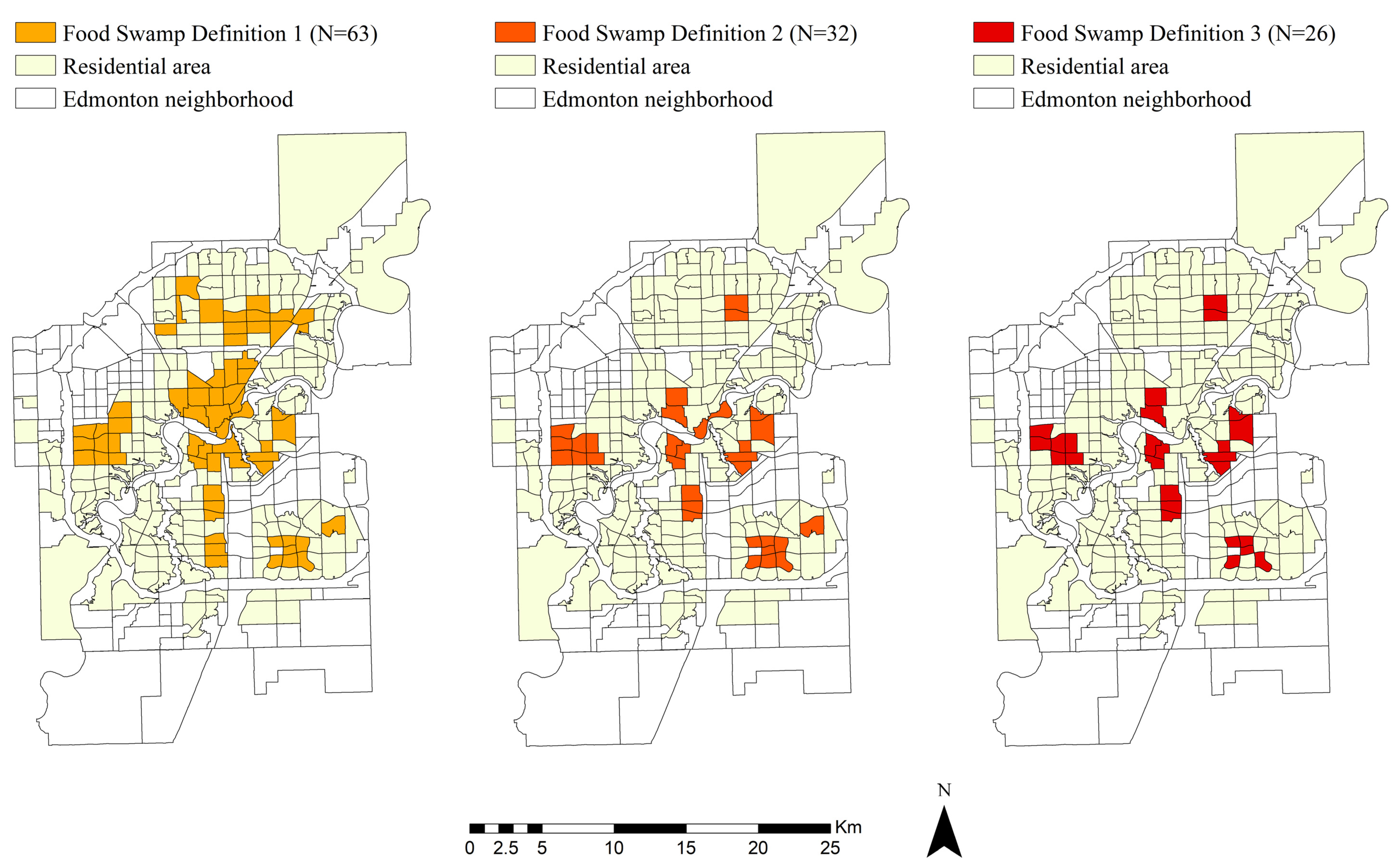
4.1. Distribution of Food Swamps

Based on our three definitions of food swamps, we found 63, 32, and 26 food swamp neighborhoods in Edmonton, respectively. The distribution of food swamps in Edmonton with different definitions is shown in Figure 4. The food swamp neighborhoods based on Definition 1 are relatively spread out over Edmonton, excluding the southwest part of the city. Food swamps based on Definitions 2 and 3 are highly coincident and clustered in certain parts of the city, including the Downtown area, the University area, the Western region, and the Southeast part of the city. According to Definitions 1 to 3, about 29.56%, 14.37%, and 11.84% of the total population resides in these food swamps, respectively.

4.2. Estimation Results of Spatial Hedonic Pricing Models

The Moran’s I, LM, and the robust LM test results for the three definitions of food swamps are presented in

Table 2. Moran’s I test and Lagrange Multiplier test statistics for the three definitions of food swamps using different weights matrix.

	Nearest 5 Weights	Nearest 10 Weights	Nearest 20 Weights	Queen Weights
	Food Swamp Definition 1
Moran test	0.271 ***	0.242 ***	0.220 ***	0.260 ***
LM-lag test	1293.4 ***	1415.9 ***	1533.3 ***	1349.7 ***
LM-error test	1709.1 ***	2649.2 ***	4350.8 ***	1612.5 ***
Robust-LM lag test	243.7 ***	234.5 ***	241.7 ***	294.7 ***
Robust-LM error test	659.5 ***	1469.7 ***	3059.2 ***	557.5 ***
	Food Swamp Definition 2
Moran test	0.269 ***	0.239 ***	0.218 ***	0.257 ***
LM-lag test	1278.3 ***	1396.3 ***	1507.4 ***	1333.3 ***
LM-error test	1674.5 ***	2589.6 ***	4259.9 ***	1578.6 ***
Robust-LM lag test	245.2 ***	235.8 ***	240.1 ***	296.1 ***
Robust-LM error test	641.5 ***	1429.0 ***	2992.6 ***	541.4 ***
	Food Swamp Definition 3
Moran test	0.269 ***	0.240 ***	0.219 ***	0.258 ***
LM-lag test	1286.0 ***	1405.6 ***	1519.8 ***	1340.3 ***
LM-error test	1684.7 ***	2612.4 ***	4304.3 ***	1589.6 ***
Robust-LM lag test	246.6 ***	236.2 ***	241.1 ***	296.8 ***
Robust-LM error test	645.3 ***	1443.1 ***	3025.5 ***	546.1 ***

Note: Significance denoted by *** p < 0.01.

. All tests significantly reject the null hypothesis of spatial independence. Given the evidence that spatial models are desirable, we estimated the SAR, SEM, and SAC models using the maximum likelihood approach and further run LR tests to choose an appropriate one among them. The test results (presented at the bottom of

Table 3. Estimation results of the SAC models for food swamps using the nearest 10 weights.

	Food Swamp	Food Swamp	Food Swamp
	Definition 1	Definition 2	Definition 3
Food Environment Type
Food swamp	−0.003	0.019 **	0.022 **
	(0.007)	(0.008)	(0.009)
Structural Variables
Log(Living area)	0.479 ***	0.479 ***	0.479 ***
	(0.008)	(0.008)	(0.008)
Log(Lot size)	0.100 ***	0.100 ***	0.100 ***
	(0.004)	(0.004)	(0.004)
Bedroom	−0.027 ***	−0.027 ***	−0.027 ***
	(0.003)	(0.003)	(0.003)
Bathroom	0.025 ***	0.025 ***	0.025 ***
	(0.003)	(0.003)	(0.003)
House condition d1	0.133 ***	0.131 ***	0.131 ***
	(0.028)	(0.028)	(0.028)
House condition d2	0.183 ***	0.182 ***	0.182 ***
	(0.029)	(0.029)	(0.029)
House condition d3	0.155 ***	0.154 ***	0.154 ***
	(0.028)	(0.028)	(0.028)
Basement condition d1	0.022 ***	0.022 ***	0.022 ***
	(0.005)	(0.005)	(0.005)
Basement condition d2	0.088 ***	0.088 ***	0.088 ***
	(0.004)	(0.004)	(0.004)
Garage	0.090 ***	0.090 ***	0.090 ***
	(0.003)	(0.003)	(0.003)
House age	−0.004 ***	−0.004 ***	−0.004 ***
	(0.000)	(0.000)	(0.000)
House age2	0.000 ***	0.000 ***	0.000 ***
	(0.000)	(0.000)	(0.000)
Locational Variables
Log (River)	−0.039 ***	−0.039 ***	−0.039 ***
	(0.004)	(0.004)	(0.004)
Log (Downtown)	0.038 ***	0.038 ***	0.037 ***
	(0.014)	(0.014)	(0.014)
Log (University)	−0.206 ***	−0.203 ***	−0.201 ***
	(0.015)	(0.015)	(0.015)
Log (Hospital)	0.010	0.011 *	0.010
	(0.006)	(0.006)	(0.006)
Log (Park)	0.002 ***	0.002 ***	0.002 ***
	(0.000)	(0.000)	(0.000)
Neighborhood Socioeconomic Status
Log (Population density)	−0.025 ***	−0.027 ***	−0.026 ***
	(0.007)	(0.007)	(0.007)
Children	0.041	0.061	0.054
	(0.086)	(0.085)	(0.085)
Senior	0.120 ***	0.121 ***	0.116 **
	(0.046)	(0.046)	(0.046)
High education	0.267 ***	0.273 ***	0.273 ***
	(0.039)	(0.039)	(0.039)
Unemployment	−0.291 ***	−0.283 ***	−0.290 ***
	(0.097)	(0.096)	(0.096)
Control variables
Season	0.011 ***	0.011 ***	0.012 ***
	(0.003)	(0.003)	(0.003)
Year 2016	−0.034 ***	−0.034 ***	−0.034 ***
	(0.003)	(0.003)	(0.003)
Year 2017	−0.061 ***	−0.061 ***	−0.061 ***
	(0.004)	(0.004)	(0.004)
Constant	7.897 ***	7.868 ***	7.863 ***
	(0.238)	(0.236)	(0.236)
Observation	8241	8241	8241
Rho (ρ)	0.177 ***	0.177 ***	0.177 ***
Lambda (λ)	0.489 ***	0.485 ***	0.486 ***
AIC	−10,982.39	−10,987.54	−10,987.87
BIC	−10,771.88	−10,777.04	−10,777.37
Log likelihood	5521.19	5523.77	5523.94
LR test (Ho: λ = 0)	429.36 ***	420.11 ***	422.54 ***
LR test (Ho: ρ = 0)	78.47 ***	79.38 ***	79.28 ***

Note: Significance denoted by *** p < 0.01, ** p < 0.05.

) suggest that SAC models cannot be simplified into SAR or SEM models. Therefore, we mainly discuss the results from SAC models in Table 3. In addition, only the results associated with the nearest 10 weights matrix are presented, because using this matrix to estimate models generates the highest log-likelihood values. When we use other k-nearest criteria (e.g., k = 5, 20) and queen criterion to define neighbors, the estimated coefficients from spatial models are similar. They have the same signs as the results showed in Table 3.

Overall, most of the estimated coefficients remain relatively stable under the three definitions of food swamps. In SAC models regarding neighborhood unhealthy food environments, the results indicate that living in food swamps generated from Definition 1 is not significantly associated with housing prices. When we consider food swamps with a low level of healthy food ratio and a high rate of low-income groups, living in food swamps has a positive and statistically significant influence on housing prices.

Concerning house structural variables, our findings show that almost all the characteristics are significantly correlated with housing prices. Specifically, living areas, lot sizes, the number of bathrooms, good house conditions, good basement conditions, and the capacity of garages are found to have positive impacts on housing prices [25,45].

Locational variables have significant impacts on housing prices by influencing residents’ living environment. Results indicate that proximity to River and University significantly increases housing prices. This is because houses with good access to River and University offer residents more opportunities to enjoy natural landscape resources and public facilities such as sports venues [32]. Furthermore, housing prices increase when a house has more extensive areas of parks within its 200-m buffer. This is because parks can bring recreational and aesthetic value to nearby residents [45,62]. On the contrary, living close to Downtown decreases housing prices. Distance to the nearest hospital hurts housing values. People are unwilling to pay extra to live very close to Downtown and hospitals because these facilities may bring traffic and sirens to nearby neighborhoods [45,61].

For neighborhood socioeconomic variables, neighborhoods with high population density and high unemployment rates have relatively low housing prices. It indicates that people would not prefer to live in crowded neighborhoods and those with many unemployed individuals [63]. Moreover, we observe positive associations between housing prices and the ratio of the senior population aged 65 and over, and the ratio of residents who have postsecondary education. Finally, as for the impacts of control variables, the results show that housing prices will significantly rise if houses are sold from April to September in Edmonton.

4.3. Estimation Results of Marginal Effects and Marginal WTP

The direct, indirect, and total marginal effects of food swamps on housing prices for SAC models are reported in

Table 4. Marginal effects estimate of the SAC models for different definitions of food swamps using the nearest 10 weights.

	Direct	Indirect	Total
Food Swamp Definition 1	−0.0027	−0.0006	−0.0033
	(0.0065)	(0.0014)	(0.0079)
Food Swamp Definition 2	0.0190 **	0.0040 **	0.0230 **
	(0.0079)	(0.0017)	(0.0095)
Food Swamp Definition 3	0.0217 **	0.0046 **	0.0263 **
	(0.0090)	(0.0020)	(0.0110)

Note: Significance denoted by ** p < 0.05.

. Our results reveal that housing prices will significantly increase by 1.90% if houses are located in food swamps (Definition 2) and increase by 2.17% if they reside in food swamps (Definition 3). Meanwhile, residing in food swamps also generate positive spillover effects to nearby houses and cause surrounding housing prices to increase by 0.40% and 0.46%, respectively.

The WTP for living in food swamp neighborhoods is reported in

Table 5. WTP estimates for different definitions of food swamps using the nearest 10 weights.

	Direct WTP	Indirect WTP	Total WTP
Food Swamp Definition 1	−1509.40	−319.42	−1827.77
Food Swamp Definition 2	10,755.70 **	2259.53 **	13,067.97 **
Food Swamp Definition 3	12,309.01 **	2583.62 **	14,961.65 **

Note: Significance denoted by ** p < 0.05.

. The results show that people are willing to pay a premium to reside in food swamp neighborhoods under Definitions 2 and 3. A typical household is willing to pay 10,755.70 CAD or 12,309.01 CAD (for Definition 2 or 3) to reside in a food swamp neighborhood. Additionally, indirect WTP indicates that nearby families are willing to pay a total of 2259.53 CAD or 2583.62 CAD (for Definition 2 or 3) to live nearby a swamp neighborhood.

5. Discussion

Our estimation results based on spatial HPMs show that people are willing to pay a premium to live in a food swamp neighborhood with the constraints of low healthy outlets ratio and/or low income level. Linking back to Figure 1, our results indicate that, overall, there is a net benefit associated with residing close to food swamps. The positive WTP reflects one or more of the three benefits/values related to fast food consumption: affordability, convenience, and taste. The first possible benefit of residing in food swamps is that households, especially low-income families, can save food costs from locating close to fast food suppliers. The food cost per household in Alberta was around 9864 CAD on average in 2017 [64], which takes up a large proportion of household annual disposable income, especially for low-income households. Nutrient-dense diets are relatively expensive, while high energy density diets are comparably cheaper per calorie base [29,65]. Thus, for low-income households, choosing and consuming fast foods and energy-dense foods may be an essential strategy for them to stretch their limited food budgets and allow them to have enough energy consumption at a lower cost. The second reason is that people value convenience and time saving from fast-food consumption. Many families, especially if both couples have jobs, may not have the luxury to spend lots of time cooking after a busy working day. The waiting and dining time are usually long in a regular restaurant. Fast food becomes a good option as it saves time for both cooking and serving. The third explanation is the preference for the taste of fast foods. Studies have found that energy-dense foods are generally more palatable and can provide more sensory enjoyment [29]. Because of the taste, studies also have observed that when low-income families spend extra money on food, they choose to buy more energy-dense unhealthy foods other than nutritional foods [29,30,66].

Based on our results, policy actions such as banning new fast-food restaurants or limiting the density of unhealthy food outlets alone may not be an efficient and effective strategy, especially in food swamp neighborhoods with the constraints of low healthy outlets ratios or/and low-income level, because for some people, such restriction on unhealthy food outlets may reduce their convenience and enjoyment brought by shopping and consuming at these places. In the long run, people can adjust by moving to somewhere else, which may reduce the effectiveness of the policy.

Moreover, these interventions may negatively impact local housing prices through people’s negative WTP and may further affect municipal revenue through property taxes. Therefore, the government may want to design alternative strategies to encourage a healthy diet and improve the food environment. First, instead of directly restricting unhealthy food outlets in food swamp neighborhoods, the local government may limit the number of unhealthy food advertisements in public areas (e.g., school areas and transportation systems) and encourage healthy food advertisements. In addition, enhancing food literacy education in communities and schools with the help of emerging media shall be helpful. Second, the City of Edmonton could support healthy food outlets such as farmers’ markets in the food swamps and grant more land for community vegetable gardens to improve healthy food access. Third, for low-income households, the local government could subsidize their purchase and consumption of healthy food, subsidize their public transport costs for grocery shopping, and provide healthy food vouchers. These efforts could work together to provide residents with incentives to change behaviors and eat more healthily.

6. Conclusions

In this study, we utilized spatial HPMs to estimate the impacts of food swamps on housing prices and examine people’s marginal WTP for residing in food swamps. Our main finding is that people are willing to pay extra to live in a food swamp neighborhood when taking low healthy-to-unhealthy food ratios and low income level into consideration. Specifically, a household is willing to pay a premium of 12,309 CAD to reside in a food swamp neighborhood with the constraints of low healthy outlets ratios and low income level. The potential reasons for the positive WTP may include the unaffordability of healthy diets and preference for the better tastes of unhealthy foods. These findings can help policymakers evaluate the effectiveness of relevant policies and develop targeted strategies to improve the local food environment.

Our investigation is based on revealed preference. People’s behaviors and preferences are often complex and diverse. Our results and explanations have contributed to an overall understanding of people’s choices and WTP for changing food environments. However, to better understand the food consumption preferences of specific populations (such as low-income people and double-employed couples with young children), more targeted and in-depth research will be required in the future. Well-designed survey studies, combined with focus group meetings, shall help.

Finally, this study has several limitations. First, there might be a potential reverse-causality issue in the hedonic price regression estimation. The property values are affected by the local food environment; however, the local food environment may also be dependent on nearby property values. For example, “unhealthy food stores” may choose to locate in neighborhoods with more low-income populations, and household income is highly correlated with property values. Given that appropriate instrumental variables can be found, future work shall find it helpful to re-estimate the WTP after controlling for potential endogeneity.

Furthermore, there is also a possibility that our analysis might suffer from selection bias. Households self-selected into food swamp neighborhoods and the unobserved error term in the location decision may be correlated with one or more missing variables in the hedonic price equation. For this selection problem, future research may consider adopting an endogenous switching regression model that allows unobserved error terms in housing selection to be correlated with unobserved errors in the hedonic equation.

References

1. Agha, M.; Agha, R. The rising prevalence of obesity: Part A: Impact on public health. Int. J. Surg. Oncol. 2017, 2, e17. [Google Scholar] [CrossRef] [PubMed] [Green Version]
2. Athens, J.K.; Duncan, D.T.; Elbel, B. Proximity to Fast-Food Outlets and Supermarkets as Predictors of Fast-Food Dining Frequency. J. Acad. Nutr. Diet. 2016, 116, 1266–1275. [Google Scholar] [CrossRef] [PubMed] [Green Version]
3. WHO. Obesity and Overweight. 2020. Available online: https://www.who.int/news-room/fact-sheets/detail/obesity-and-overweight (accessed on 9 November 2021).
4. Dixon, J.B. The effect of obesity on health outcomes. Mol. Cell. Endocrinol. 2010, 316, 104–108. [Google Scholar] [CrossRef] [PubMed]
5. WHO. Weight Bias and Obesity Stigma: Considerations for the WHO European Region. 2017. Available online: https://www.euro.who.int/en/health-topics/noncommunicable-diseases/obesity/publications/2017/weight-bias-and-obesity-stigma-considerations-for-the-who-european-region-2017 (accessed on 9 November 2021).
6. Afshin, A.; Sur, P.J.; Fay, K.A.; Cornaby, L.; Ferrara, G.; Salama, J.S.; Mullany, E.C.; Abate, K.H.; Abbafati, C.; Abebe, Z.; et al. Health effects of dietary risks in 195 countries, 1990–2017, a systematic analysis for the Global Burden of Disease Study 2017. Lancet 2019, 393, 1958–1972. [Google Scholar] [CrossRef] [Green Version]
7. Boumtje, P.I.; Huang, C.L.; Lee, J.Y.; Lin, B.H. Dietary habits, demographics, and the development of overweight and obesity among children in the United States. Food Policy 2005, 30, 115–128. [Google Scholar] [CrossRef]
8. Glanz, K.; Sallis, J.F.; Saelens, B.E.; Frank, L.D. Healthy nutrition environments: Concepts and measures. Am. J. Health Promot. 2005, 19, 330–333. [Google Scholar] [CrossRef]
9. Larson, N.I.; Story, M.T.; Nelson, M.C. Neighborhood environments: Disparities in access to healthy foods in the U.S. Am. J. Prev. Med. 2009, 36, 74–81. [Google Scholar] [CrossRef]
10. Kyureghian, G.; Nayga, R.M. Food Store Access, Availability, and Choice when Purchasing Fruits and Vegetables. Am. J. Agric. Econ. 2013, 95, 1280–1286. [Google Scholar] [CrossRef]
11. Morland, K.B.; Evenson, K.R. Obesity prevalence and the local food environment. Health Place 2009, 15, 491–495. [Google Scholar] [CrossRef] [Green Version]
12. Dunn, R.A.; Sharkey, J.R.; Horel, S. The effect of fast-food availability on fast-food consumption and obesity among rural residents: An analysis by race/ethnicity. Econ. Hum. Biol. 2012, 10, 1–13. [Google Scholar] [CrossRef]
13. Jekanowski, M.D.; Binkley, J.K.; Eales, J. Convenience, Accessibility, and the Demand for Fast Food. J. Agric. Resour. Econ. 2001, 26, 58–74. [Google Scholar]
14. Moore, L.V.; Diez Roux, A.V.; Nettleton, J.A.; Jacobs, D.R.; Franco, M. Fast-food consumption, diet quality, and neighborhood exposure to fast food: The multi-ethnic study of atherosclerosis. Am. J. Epidemiol. 2009, 170, 29–36. [Google Scholar] [CrossRef] [PubMed] [Green Version]
15. Fitzpatrick, K.; Greenhalgh-Stanley, N.; Ver Ploeg, M. Food deserts and diet-related health outcomes of the elderly. Food Policy 2019, 87, 101747. [Google Scholar] [CrossRef]
16. Wang, H.; Qiu, F.; Swallow, B. Can community gardens and farmers’ markets relieve food desert problems? A study of Edmonton, Canada. Appl. Geogr. 2014, 55, 127–137. [Google Scholar] [CrossRef]
17. Cooksey-Stowers, K.; Schwartz, M.B.; Brownell, K.D. Food Swamps Predict Obesity Rates Better Than Food Deserts in the United States. Int. J. Environ. Res. Public Health 2017, 14, 1366. [Google Scholar] [CrossRef] [Green Version]
18. Hager, E.R.; Cockerham, A.; O’Reilly, N.; Harrington, D.; Harding, J.; Hurley, K.M.; Black, M.M. Food swamps and food deserts in Baltimore City, MD, USA: Associations with dietary behaviours among urban adolescent girls. Public Health Nutr. 2016, 20, 2598–2607. [Google Scholar] [CrossRef] [Green Version]
19. Luan, H.; Law, J.; Quick, M. Identifying food deserts and swamps based on relative healthy food access: A spatio-temporal Bayesian approach. Int. J. Health Geogr. 2015, 14, 37. [Google Scholar] [CrossRef] [Green Version]
20. Rose, D.D.; Bodor, J.N.; Swalm, C.M.; Rice, J.C.; Farley, T.A.; Hutchinson, P.L. Deserts in New Orleans? Illustrations of Urban Food Access and Implications for Policy; University of Michigan National Poverty Centre and the USDA Economic Research Service Research: Ann Arbor, MI, USA, 2009.
21. Alkon, A.H.; Block, D.; Moore, K.; Gillis, C.; Dinuccio, N.; Chavez, N. Foodways of the urban poor. Geoforum 2013, 48, 126–135. [Google Scholar] [CrossRef]
22. Shannon, J. Should we fix food deserts? The politics and practice of mapping food access. In Doing Nutrition Differently; Routledge: New York, NY, USA, 2016; pp. 267–294. [Google Scholar]
23. Tyvimaa, T.; Gibier, K.M.; Zahirovic-Herbert, V. The effect of ground leases on house prices in Helsinki. J. Hous. Built Environ. 2015, 30, 451–470. [Google Scholar] [CrossRef]
24. Heyman, A.V.; Sommervoll, D.E. House prices and relative location. Cities 2019, 95, 102373. [Google Scholar] [CrossRef]
25. Atreya, A.; Kriesel, W.; Mullen, J.D. Valuing Open Space in a Marshland Environment: Development Alternatives for Coastal Georgia. J. Agric. Appl. Econ. 2016, 48, 383–402. [Google Scholar] [CrossRef] [Green Version]
26. Chen, S.; Jin, H. Pricing for the clean air: Evidence from Chinese housing market. J. Clean. Prod. 2019, 206, 297–306. [Google Scholar] [CrossRef]
27. Kim, C.W.; Phipps, T.T.; Anselin, L. Measuring the benefits of air quality improvement: A spatial hedonic approach. J. Environ. Econ. Manag. 2003, 45, 24–39. [Google Scholar] [CrossRef] [Green Version]
28. Li, H.; Wei, Y.D.; Yu, Z.; Tian, G. Amenity, accessibility and housing values in metropolitan USA: A study of Salt Lake County, Utah. Cities 2016, 59, 113–125. [Google Scholar] [CrossRef]
29. Drewnowski, A.; Specter, S. Poverty and obesity: The role of energy density and energy costs. Am. J. Clin. Nutr. 2004, 79, 6–16. [Google Scholar] [CrossRef] [PubMed]
30. Banerjee, A.V.; Duflo, E. Poor Economics: A Radical Rethinking of the Way to Fight Global Poverty; Public Affairs: New York, NY, USA, 2011. [Google Scholar]
31. Anselin, L.; Gallo, J.L. Interpolation of Air Quality Measures in Hedonic House Price Models: Spatial Aspects. Spat. Econ. Anal. 2006, 1, 31–52. [Google Scholar] [CrossRef]
32. Schläpfer, F.; Waltert, F.; Segura, L.; Kienast, F. Valuation of landscape amenities: A hedonic pricing analysis of housing rents in urban, suburban and periurban Switzerland. Landsc. Urban Plan. 2015, 141, 24–40. [Google Scholar] [CrossRef]
33. Cao, Y.; Swallow, B.; Qiu, F. Identifying the effects of a land-use policy on willingness to pay for open space using an endogenous switching regression model. Land Use Policy 2021, 102, 105183. [Google Scholar] [CrossRef]
34. Bark, R.H.; Osgood, D.E.; Colby, B.G.; Halper, E.B. How Do Homebuyers Value Different Types of Green Space? J. Agric. Resour. Econ. 2011, 36, 395–415. [Google Scholar]
35. Lin, W.; Tou, J.C.; Lin, S.Y.; Yeh, M.Y. Effects of socioeconomic factors on regional housing prices in the USA. Int. J. Hous. Mark. Anal. 2014, 7, 30–41. [Google Scholar] [CrossRef]
36. Saphores, J.D.; Li, W. Estimating the value of urban green areas: A hedonic pricing analysis of the single family housing market in Los Angeles, CA. Landsc. Urban Plan. 2012, 104, 373–387. [Google Scholar] [CrossRef]
37. D’Elia, V.V.; Grand, M.C.; León, S. Bus rapid transit and property values in Buenos Aires: Combined spatial hedonic pricing and propensity score techniques. Res. Transp. Econ. 2020, 80, 100814. [Google Scholar] [CrossRef]
38. Mueller, J.M.; Loomis, J.B. Spatial Dependence in Hedonic Property Models: Do Different Corrections for Spatial Dependence Result in Economically Significant Differences in Estimated Implicit Prices? J. Agric. Resour. Econ. 2008, 33, 212–231. [Google Scholar]
39. Osseni, A.F.; Bareille, F.; Dupraz, P. Hedonic valuation of harmful algal bloom pollution: Why econometrics matters? Land Use Policy 2021, 107, 104283. [Google Scholar] [CrossRef]
40. LeSage, J.; Pace, R.K. Introduction to Spatial Econometrics; Chapman and Hall/CRC: New York, NY, USA, 2009. [Google Scholar]
41. Bockstael, N.E.; McConnell, K.E. Environmental and Resource Valuation with Revealed Preferences: A Theoretical Guide to Empirical Models; Springer Science & Business Media: Dordrecht, The Netherlands, 2007. [Google Scholar]
42. City of Edmonton. 2019 Municipal Census Results. 2019. Available online: https://www.edmonton.ca/city_government/facts_figures/municipal-census-results.aspx (accessed on 9 November 2021).
43. Health Quality Council of Alberta. Overweight & Obesity in Adult Albertans: A Role for Primary Healthcare. 2015. Available online: https://hqca.ca/news/2015/07/overweight-obesity-in-adult-albertans-a-role-for-primary-healthcare/ (accessed on 9 November 2021).
44. City of Edmonton. Fresh—Edmonton’s Food and Urban Agriculture Strategy. 2012. Available online: http://www.edmonton.ca/city_government/documents/FRESH_October_2012.pdf (accessed on 9 November 2021).
45. Li, H.; Wei, Y.D.; Wu, Y.; Tian, G. Analyzing housing prices in Shanghai with open data: Amenity, accessibility and urban structure. Cities 2019, 91, 165–179. [Google Scholar] [CrossRef]
46. Freeman, A.M., III; Herriges, J.A.; Kling, C.L. The Measurement of Environmental and Resource Values: Theory and Methods, 3rd ed.; Routledge: New York, NY, USA, 2014. [Google Scholar]
47. Statistic Canada. Consumer Price Index, Annual Average, Not Seasonally Adjusted. 2017. Available online: https://www150.statcan.gc.ca/t1/tbl1/en/tv.action?pid=1810000501&pickMembers%5B0%5D=1.23 (accessed on 9 November 2021).
48. City of Edmonton’s Business Licenses Database. 2018. Available online: https://data.edmonton.ca/Sustainable-Development/City-of-Edmonton-Business-Licenses/qhi4-bdpu/data (accessed on 9 November 2021).
49. Block, J.P.; Scribner, R.A.; DeSalvo, K.B. Fast food, race/ethnicity, and income. Am. J. Prev. Med. 2004, 27, 211–217. [Google Scholar] [CrossRef]
50. Lee, H. The role of local food availability in explaining obesity risk among young school-aged children. Soc. Sci. Med. 2012, 74, 1193–1203. [Google Scholar] [CrossRef]
51. Li, M.; Ashuri, B. Neighborhood racial composition, neighborhood wealth, and the surrounding food environment in Fulton County, GA. Appl. Geogr. 2018, 97, 119–127. [Google Scholar] [CrossRef]
52. Kolak, M.; Bradley, M.; Block, D.R.; Pool, L.; Garg, G.; Toman, C.K.; Boatright, K.; Lipiszko, D.; Koschinsky, J.; Kershaw, K.; et al. Urban foodscape trends: Disparities in healthy food access in Chicago, 2007–2014. Health Place 2018, 52, 231–239. [Google Scholar] [CrossRef]
53. Wang, H.; Qiu, F. Fresh food access revisited. Cities 2016, 51, 64–73. [Google Scholar] [CrossRef]
54. Yang, M.; Wang, H.; Qiu, F. Neighbourhood food environments revisited: When food deserts meet food swamps. Can. Geogr. 2020, 64, 135–154. [Google Scholar] [CrossRef]
55. City of Edmonton. North Saskatchewan River. 2020. Available online: https://www.edmonton.ca/activities_parks_recreation/parks_rivervalley/north-saskatchewan-river.aspx (accessed on 9 November 2021).
56. Alberta Government. Upper North Saskatchewan and Red Deer River Study Area. 2018. Available online: https://open.alberta.ca/opendata/gda-0a12e487-75a6-4198-8ed2-67872ff20ac6 (accessed on 9 November 2021).
57. Downtown Business Association. Shopping & Dining. 2020. Available online: https://www.edmontondowntown.com/shopping-dining/ (accessed on 9 November 2021).
58. University of Alberta. 2020. Available online: https://www.ualberta.ca/about/facts.html. (accessed on 9 November 2021).
59. City of Edmonton Open Data Catalogue. 2016. Available online: https://data.edmonton.ca/Thematic-Features/City-of-Edmonton-Zoning-Bylaw-Map/b4f2-gf2b#revert (accessed on 9 November 2021).
60. City of Edmonton Open Data Catalogue. 2018. Available online: https://data.edmonton.ca/browse?q=2016%20census&sortBy=relevance (accessed on 9 November 2021).
61. Tian, G.; Wei, Y.D.; Li, H. Effects of accessibility and environmental health risk on housing prices: A case of Salt Lake County, Utah. Appl. Geogr. 2017, 89, 12–21. [Google Scholar] [CrossRef]
62. Netusil, N.R. Urban environmental amenities and property values: Does ownership matter? Land Use Policy 2013, 31, 371–377. [Google Scholar] [CrossRef]
63. Li, W.; Joh, K.; Lee, C.; Kim, J.H.; Park, H.; Woo, A. Assessing Benefits of Neighborhood Walkability to Single-Family Property Values. J. Plan. Educ. Res. 2015, 35, 471–488. [Google Scholar] [CrossRef]
64. Statistics Canada. Detailed Food Spending, Canada, Regions and Provinces. 2021. Available online: https://www150.statcan.gc.ca/t1/tbl1/en/tv.action?pid=1110012501&pickMembers%5B0%5D=1.12&cubeTimeFrame.startYear=2015&cubeTimeFrame.endYear=2019&referencePeriods=20150101%2C20190101 (accessed on 9 March 2022).
65. Maillot, M.; Darmon, N.; Vieux, F.; Drewnowski, A. Low energy density and high nutritional quality are each associated with higher diet costs in French adults. Am. J. Clin. Nutr. 2007, 86, 690–696. [Google Scholar] [PubMed]
66. Jensen, R.T.; Miller, N.H. Giffen Behavior and Subsistence Consumption. Am. Econ. Rev. 2008, 98, 1553–1577. [Google Scholar] [CrossRef]
Figure 1. Framework of the relationship between food swamps and willingness to pay for living in food swamps.
Sustainability 14 05961 g001
Figure 2. Edmonton Map.
Sustainability 14 05961 g002
Figure 3. Distribution of Property Values in Edmonton.
Sustainability 14 05961 g003
Figure 4. Distribution of Food Swamps Based on Three Different Definitions.
Sustainability 14 05961 g004