Article

A Robust Adaptive Traffic Signal Control Algorithm Using Q-Learning under Mixed Traffic Flow

1
College of Information and Computer Engineering, Northeast Forestry University, Harbin 150040, China
2
School of Traffic and Transportation, Northeast Forestry University, Harbin 150040, China
*
Author to whom correspondence should be addressed.
These authors contributed equally to this work.
Sustainability 2022, 14(10), 5751; https://doi.org/10.3390/su14105751
Submission received: 12 April 2022 / Revised: 5 May 2022 / Accepted: 7 May 2022 / Published: 10 May 2022

Abstract

:
The operational and safety performance of intersections is the key to ensuring the efficient operation of urban traffic. With the development of automated driving technologies, the ability of adaptive traffic signal control has been improved according to data detected by connected and automated vehicles (CAVs). In this paper, an adaptive traffic signal control was proposed to optimize the operational and safety performance of the intersection. The proposed algorithm based on Q-learning considers the data detected by loop detectors and CAVs. Furthermore, a comprehensive analysis was conducted to verify the performance of the proposed algorithm. The results show that the average delay and conflict rate have been significantly optimized compared with fixed timing and traffic actuated control. In addition, the performance of the proposed algorithm is good in the test of the irregular intersection. The algorithm provides a new idea for the intelligent management of isolated intersections under the condition of mixed traffic flow. It provides a research basis for the collaborative control of multiple intersections.

1. Introduction

Traffic signal control is widely studied as an effective means to improve the operational and safety performance of intersections. Traffic control systems can be roughly divided into three types: fixed timing (FT), traffic actuated control (TAC), and adaptive traffic signal control (ATSC). Recent research focuses on ATSC, while the other two control algorithms are mainly used as the research baseline [1]. ATSC needs a lot of accurate data to optimize the operational and safety performance of intersections in real-time [2].
The traffic flow data required by traditional TAC and ATSC are usually collected by loop detectors, which is a common and economical method at present [3]. With the development of connected and automated vehicles (CAVs), the way ATSC obtains real-time data have been expanded compared with human-driven vehicle (HDV) [4,5,6,7]. Existing studies generally believe that only CAV data can realize intelligent vehicle infrastructure cooperative systems [8,9,10]. Yet, Yang et al. [11] found that the integration of loop detectors data and CAVs data can improve the performance of traffic control algorithms. In addition, as mentioned above, the loop detector is widely used, and it is feasible and economical to integrate its data with CAVs data in the proposed traffic control algorithm. However, it can be considered that the data collected by the loop detector at a low market penetration rate (MPR) is more accurate than CAVs data, and the conclusion is the opposite at a high MPR. Therefore, how to balance them is a crucial problem in traffic signal control.
In the development and researches of ATSC, various algorithms, such as heuristic algorithm and reinforcement learning, are applied to improve the operational and safety performance of intersections [12]. Among all algorithms, the Q-learning algorithm has been widely studied and achieved satisfactory performance [13,14,15]. Guo and Harmati [16] proposed an ATSC based on Q-learning and considered Nash equilibriums to improve traffic control performance at intersections. Abdoos et al. [17] presented a two-level hierarchical control of traffic signals based on Q-learning, and the results show that the proposed hierarchical control improves the Q-learning efficiency of the bottom level agents. Wang et al. [18] proposed a multi-agent reinforcement learning traffic control system based on Q-learning, and the results show that their algorithm outperforms the other multi-agent reinforcement learning algorithms in terms of multiple traffic metrics. Their research provides an idea for testing ATSC based on Q-learning, that is, comprehensive analysis from multiple perspectives. In addition, the model of reward function in Q-learning is the key to the implementation of the algorithm, that is, the optimization object. Essa and Sayed [19] designed an ATSC based on Q-learning to optimize the conflict rate. However, their algorithm requires a large amount of complex data and is not suitable for low-level detectors (such as loop detectors). Abdoos [20] proposed an ATSC with the object of optimizing the queue length and achieved good results in the simulation. The queue length used in her algorithm is the traffic data that the existing detectors can collect. However, the algorithm lacks comprehensive analysis, such as testing under different traffic demands and unbalanced traffic flow.
The existing research on intersection optimization attempts to improve the operation and safety performance at the same time [19,21,22]. In recent years, robustness testing has been widely used in the research of traffic control [23,24,25]. At the same time, the impact of unbalanced traffic flow on the operation and safety performance of intersections has also been widely concerned by scholars [26]. In addition, the test of traffic control at irregular intersections has been proved necessary [27]. Thus, comprehensive tests need to be carried out in the above environment to make the research more convincing.
To fill the above gaps, we proposed an ATSC based on a Q-learning algorithm that integrates data obtained by existing loop detectors and CAVs. In addition, a comprehensive analysis was conducted to test the performance of the proposed algorithm in various traffic conditions.

2. Algorithm Design

In this section, we designed an ATSC algorithm using Q-learning to optimize the operational performance of intersections in terms of the data obtained by loop detectors and CAVs. Specifically, the queue length estimated by loop detectors and CAVs is the optimized objective to enhance the operational and safety performance of intersections. The general flow of the proposed algorithm is represented in Figure 1. As shown in the figure, loop detectors or CAVs collect data during the operation of the current cycle. When the cycle ends, the Q-learning algorithm is conducted to calculate the signal timing of the next cycle. So back and forth.
Q-learning is a value-based algorithm in the reinforcement learning algorithms. Q is Q ( s , a ) , which is the expectation that taking action a in the state s at a certain time can obtain income. The environment will feedback the corresponding reward r according to the action of the agent. Therefore, the main idea of the algorithm is to build states and actions into a q-table to store the Q value and then select the action that can obtain the maximum income according to the Q value. Q-learning is one of reinforcement learning algorithms, and the process of it can be as follows:
Q N e w ( s t , a t ) = Q ( s t , a t ) + α R ( s t , a t ) + γ max a A Q ( s t + 1 , a t + 1 ) Q ( s t , a t )
where Q N e w ( s t , a t ) is the update Q value; Q ( s t , a t ) is the Q value which selected action a t under state s t in the last episode; α is the learning rate; R ( s t , a t ) is the reward under ( s t , a t ) ; γ is the discount rate and it is 0.7 in this study; A is the set of actions; Q ( s t + 1 , a t + 1 ) is the Q value in next step.

2.1. State Representation

In the Q-learning algorithm, states are constantly changing according to the choice of actions. Therefore, each loop in Q-learning needs to redefine the current state. As mentioned above, the order of queue length of each approach in the intersection estimated by loop detectors and CAVs is used as the state set. In this study, the state set is presented in Table 1, which is the same as [
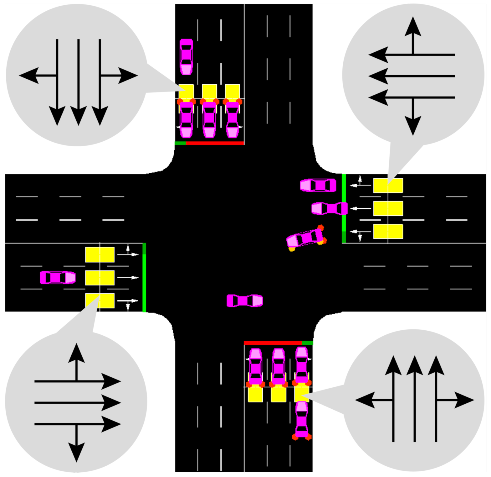
20]. Firstly, we number the approaches. Specifically, we take the four-legs intersection as an example, and the number of each approach is 1–4. q l is the queue length in the l-th approach. After selecting each action, the queue length of each approach is sorted to correspond to each state in Table 1. A boundary state is needed to make the program break in Q-learning, and three constraints are set in this study. When the queue length of two approaches under the red phase is higher than the others simultaneously, or one of the queue lengths is higher than the length of the lane, the current state is marked as terminal. In addition, The selection of action is limited by the maximum green time, as shown below.

2.2. Action Representation

There are 200 loops in the proposed algorithm to search for the optimal scheme. It needs to keep adjusting the signal timing until the current state is terminal. During each time step of one loop, two actions can be chosen to adjust the current signal timing as follows:
A = 1 , q l L l 0 , q l > L l
where, L l is the length of the l lane.
Specifically, actions can be selected 1 or 0, representing the extension time (1 s or 0 s). In other words, the current green time could be extended to 1 s or 0 s if the respective condition is true. However, the queue length estimated by loop detectors and low MPR CAVs is inaccurate, so we adjust the reward function in the next section to improve accuracy. In this study, the maximum cycle is 120 s, and the minimum green time is 20 s, so the maximum green time is set to 100 s.

2.3. Reward Function

As mentioned, the proposed algorithm aims to improve the performance of intersections according to the queue length of each approach. In each loop, the proposed algorithm predicts the queue length of each approach in the time step, which uses the data detected by loop detectors and CAVs as the initial state. The queue length of each approach can be estimated as follows:
q ( l ) = 1 n 1 ( L v ( i ) + g ( i ) ) + L v ( n )
where, q ( l ) is the queue length of the l lane; n is the number of vehicles in queue. L v ( i ) is the length of the i-th vehicle; g ( i ) is the gap between the i-th and the i + 1 -th vehicle.
Furthermore, the number of vehicles in queue n is inaccurate when estimated by loop detectors and CAVs under low MPRs. As Equation (4) shows that the traffic flow m is the key parameter to calculate n. However, m detected by loop detectors could not adapt to the real-time traffic demand. In addition, there is limited data to calculate m under low MPRs.
n = 0 t r m t · I ( p P R ) d t
where t r is the red time; m is the traffic flow per second; I ( · ) is the selection function, and if the p P R is true, the value is 1; p is the current phase; P R is the set of red phase.
In the prediction process, the green time and red time of each phase change one after another. The duration of the red phase will increase with the increase in the green time. Thus, the red time t r can be determined as follows:
t r = G m i n + t
where, G m i n is the minimum green time, it is 20 s in this study; t is the time step, and it is 1 s due to the selection of actions mentioned above.
The queue length detected by two methods is conducted in the reward function to enhance the accuracy. Under low MPR, there are few CAVs in intersections, and the amount of data detected is not enough, resulting in insufficient accuracy. At this time, it is wise to predict the queue length through the loop detector data rather than CAV. On the other hand, when high MPR is reached, the amount and accuracy of data detected by CAVs will meet the demand, making the predicted queue length more accurate than loop detectors. Therefore, we can conclude that the key to algorithm ability lies in MPR. In this study, we proposed a reward function to adjust the weight of the two methods through MPR as follows:
R ( s t , a t ) = i = 1 n ( ( 1 ε ) q i + ε q i )
where R ( s t , a t ) is the value of reward at ( s t , a t ) ; q i is the queue length estimated by the loop detector; q i is the queue length detected by CAVs; ε is the current MPR.

3. Simulations and Results

3.1. Simulation Settings

3.1.1. Intersection Geometry

In this section, the operational and safety performance of the proposed algorithm is verified through the Simulation of Urban Mobility (SUMO). We set up a virtual orthogonal intersection with four legs in SUMO (see Figure 2). Each approach has three lanes, and two loop detectors are set at the beginning and end of each lane. Note that the detectors at the end of each lane are used to test the performance of the intersection. Additionally, others are conducted to collect data for the proposed algorithm. Moreover, each lane is 250 m, and we took the geometric center of the intersection as a circle point with a radius of 250 ft as the detection area just as [28,29].

3.1.2. Traffic Demand

We set a balance traffic demand at each approach with 1000 veh/h to test the performance between the proposed algorithm and baselines (FT and TAC). Note that the traffic demand set in SUMO is not fixed in each approach but the base of traffic volume. In other words, the traffic demand per approach (1000 veh/h) means that the number of random vehicles is generated based on 1000 veh/h in SUMO. The high and unbalanced traffic flow is set in the next section. In this study, we focus on the algorithm performance in the case of two phases, so the proportion of left turn and right turn vehicles is set to 10%, respectively.

3.1.3. Vehicle Types

In total, 11 MPRs (from 0 to 100%) are placed in SUMO to simulate the mixed traffic flow. As mentioned in the introduction, the IDM and CACC are the car-following models of HDV and CAV. Since the intersection is virtual, the default parameters are acceptable for conducting simulations.

3.1.4. Baselines

The baselines of this study include FT and TAC, where FT is calculated according to the method described in HCM [30], and TAC adopts the program provided in SUMO [31]. In order to make the comparison more convincing, the parameters of FT and TAC are consistent with the proposed algorithm: the maximum cycle is 120 s, and the minimum green time is 20 s.

3.2. Simulation Results

3.2.1. Operational Performance of the Proposed Algorithm

The operational performance is verified through the average delay in this study. Delay is defined as the difference between the current travel time since a vehicle enters the incoming lane of the intersection and the expected minimum travel time of the lane l. Average delay D ¯ is calculated as Equations (7) and (8).
t m i n ( l ) = L ( l ) v m a x ( l )
where t m i n ( l ) is the minimum travel time for vehicles at lane l; L ( l ) is the length of the lane l; v m a x ( l ) is the maximum speed at the lane l, and the value of it is limited speed in this study.
D ¯ = v V ( l , t ) ( t t 0 ( v , l ) t m i n ( l ) ) n v
where V ( l , t ) is the set of all vehicles in lane l at time t; t is current time step; t 0 ( v , l ) is the time step when vehicle v arrives at lane l.
Figure 3 shows the average delay under various MPRs using FT, TAC, and the proposed algorithm. It can be clearly found that the operational performances of TAC and the proposed algorithm are better than FT. In the numerical experiment, the average delay of the proposed algorithm reduces by 9.1–16.9% than FT. The optimized performance is significant under high MPRs (more than 50%). In addition, it can be seen that the average delay of the proposed algorithm reduces significantly than TAC under high MPRs. Yet, compared with TAC, the average delay of the proposed algorithm even increases in some low MPRs than TAC. It could be explained that the operational performance is not significantly optimized between the proposed algorithm and TAC under low MPRs in common traffic flow scenarios. We will verify this hypothesis in the next section.
The differences in the average delay under various MPRs using the proposed algorithm compared with FT and TAC are integrated into Table 2. It can be clearly found that the optimizations of the average delay using the proposed algorithm under various MPRs are significant compared with FT. However, the optimizations compared with TAC are not as well as that of FT. Significantly, the performance of the average delay is worse under 30% and 40% MPR. The optimization effect is relatively stable when the MPR is higher than 50%.

3.2.2. Safety Performance of the Proposed Algorithm

The safety performance is estimated by conflict rate according to Time-to-Collision (TTC) in this study. TTC can be calculated as Equation (9). In general, a conflict can be marked when the TTC is lower than 1.5 s. Recently, Mousavi et al. [32] found that the TTC threshold should be different between HDVs and CAVs according to their operational characteristics. Hence, the TTC threshold of HDVs is 1.5 s and CAVs is 1 s in this study.
T T C = s l f v f v l , v f > v l
where s l f is the space between the leading vehicle and the follower; v f is the velocity of the following vehicle; v l is the velocity of the leading vehicle.
Figure 4 shows that the conflict rate of the proposed algorithm reduces than FT and TAC, especially under high MPRs. In the numerical experiment, the conflict rate of the proposed algorithm reduces by 5.2–36.3% than FT. Hence, it can be explained that the safety performance is better than FT. Moreover, it significantly reduces (25.3–34.8%) than FT under high MPRs (≥80%). Yet, the conflict rate of the proposed algorithm compared with TAC is not as significant as FT under most of MPRs.
The differences in the conflict rate under various MPRs using the proposed algorithm compared with FT and TAC are displayed in Table 3. Compared with FT, the conflict rate reduces by 29.82–36.34% when MPR is higher than 70%. Simultaneously, the performance of the conflict rate of the proposed algorithm is significant under high MPR (>70%) compared with TAC. Unlike the average delay performance, the conflict rate is always reduced under various MPRs than TAC and FT.

4. Discussion

In this section, We will comprehensively test the performance of the proposed algorithm. The tests cover robustness, unbalanced traffic flow the irregular intersection, and the impact of MPR on algorithm performance is also analyzed.

4.1. Robust Analysis

Standard traffic demand (1000 veh/h) has been used above to test the operational and safety performance of the proposed algorithm. This section will verify its robustness by enhancing traffic demand (1500 veh/h and 2000 veh/h) at each approach to simulate peak hours.
Figure 5 shows the average delay of the three control algorithms under various MPRs in 1500 veh/h and 2000 veh/h. It can be found that the optimized performances of the proposed algorithm in 1500 veh/h and 2000 veh/h are better than in 1000 veh/h. In addition, compared with FT, it can be found that the optimized performances of TAC in 1500 veh/h and 2000 veh/h are extraordinary significant than in 1000 veh/h. In the numerical experiment, the average delay of the proposed algorithm reduces by 6.3–23.2% (in 1500 veh/h) and 4.5–13.4% (in 2000 veh/h) than TAC, respectively. Compared with in 1000 veh/h, the average delay of FT increases significantly in 1500 veh/h and 2000 veh/h. Yet, this result is not found in the proposed algorithm.
The differences in the average delay under various MPRs using the proposed algorithm compared with FT and TAC both in 1500 veh/h and 2000 veh/h integrated into Table 4. It can be found that the differences in the average delay compared with FT always increase under almost all MPRs when the traffic demand rises from 1500 veh/h to 2000 veh/h. However, this conclusion is not found between TAC and the proposed algorithm. In other words, the optimization of the average delay using the proposed algorithm is more stable than TAC. Thus, it can be explained that the performance of FT deteriorates more significantly than the TAC and the proposed algorithm under high traffic demands.
Figure 6 shows the conflict rate under various MPRs using three control algorithms in 1500 veh/h and 2000 veh/h. Compared with in 1000 veh/h, the conflict rates of FT and TAC have evident fluctuations in 1500 veh/h and 2000 veh/h. Moreover, the conflict rate of the proposed algorithm reduces significantly than FT and TAC. It can be explained that the proposed algorithm has a better performance compared with baselines in high traffic demands. In the numerical experiment, the conflict rate of the proposed algorithm, respectively, reduces by 5.3–12.0% and 8.3–11.6% than FT and TAC under high MPRs (≥80%).
The differences in the conflict rate under various MPRs using the proposed algorithm compared with FT and TAC both in 1500 veh/h and 2000 veh/h are in Table 5. Similar to in 1000 veh/h, the reduction in the conflict rate using the proposed algorithm is not significant compared with FT (1.76–4.05%) and TAC (0.31–2.16%) under low MPRs (no more than 30%). In addition, it can be found that the optimized effect compared with FT and TAC in 1500 veh/h is better than in 2000 veh/h under various MPRs.

4.2. Unbalanced Flow Analysis

The previous work in this study assumes that the four approaches have the same traffic demand, but the traffic volume at intersections is often unbalanced in the real-world. Hence, we set the traffic demand of arterial approaches as 1000 veh/h, and that of branch approaches as 500 veh/h to test the performance of the proposed algorithm under unbalanced flow. In Figure 2, the two approaches in the horizontal direction are arterial approaches, and the two approaches in the vertical direction are the branch.
Figure 7 shows the average delay under various MPRs using the three control algorithms in unbalanced flow. It can be found that the average delay of the proposed algorithm has obvious low values than FT and TAC under various MPRs. It can illustrate that the operational performances of the proposed algorithm are better than baselines.
The differences in the average delay under various MPRs using the proposed algorithm compared with FT and TAC in unbalanced flow integrated into Table 6. The average delay reduces significantly compared with FT (24.28–32.12%) and TAC (16.74–30.06%), and the decline is relatively stable. That is, the optimized effect of the proposed algorithm is stable than FT and TAC under various MPRs.
Figure 8 shows the conflict rate under various MPRs using the three control algorithms in unbalanced flow. Compared with FT, the conflict rate of TAC reduces significantly from 40% to 100% MPR. This trend is the same as the average delay under unbalanced flow (see Figure 7). However, the difference in conflict rate between TAC and the proposed algorithm closes with the increase in MPR.
Table 7 lists the differences in the conflict rate under various MPRs using the proposed algorithm compared with FT and TAC in unbalanced flow. Similar to the performance of the average delay, the optimization of the proposed algorithm is significant in the conflict rate under various MPRs compared with FT. However, the conflict rate reduces relatively few under high MPRs (more than 60%) compared with TAC (3.24–19.52%). It can be explained that safety performance of TAC is satisfactory in unbalanced flow under high MPRs.

4.3. Effect of Intersection Geometry

Moreover, the effect of intersection geometry must be discussed to test the proposed algorithm. As mentioned above, we have verified the operational and safety performance at the orthogonal intersection. However, the orthogonal intersection is excessively ideal, so the proposed algorithm needs to supplement the evidence of the performance. In this section, the irregular intersection (see Figure 9) is conducted to test the performance of the proposed algorithm. Moreover, the traffic demand is set as 1000 veh/h.
Figure 10 shows the average delay under various MPRs at the irregular intersection. Obviously, the traffic capacity has been dramatically affected at the irregular intersection. Thus, the average delay using all three algorithms increases significantly compared with the aforementioned scenarios. With the increase in MPR, the average delay curves of FT and TAC fluctuate obviously, while that of the proposed algorithm is relatively stable. In addition, the reduction in the average delay using the proposed algorithm is more significant under each MPR compared with FT and TAC.
The differences in the average delay under various MPRs using the proposed algorithm compared with FT and TAC at the irregular intersection are integrated into Table 8. Compared with FT and TAC, the average delay reduction under each MPR is relatively stable. Compared with the orthogonal intersection in 1000 veh/h, the average delay between the proposed algorithm and TAC decreases. In addition, the average delay of the proposed algorithm is more than 3% lower than that of TAC. Thus, the optimized performance of the proposed algorithm at the irregular intersection is better than at the orthogonal intersection (note that the Optimized Performance is not the actual Operational Performance, it is relative to TAC).
Figure 11 shows the conflict rate under various MPRs at the irregular intersection. Similar to the average delay, the conflict rate has been dramatically affected at the irregular intersection. It can be seen that the conflict rate curve of the proposed algorithm is smoother than that of FT and TAC, and the conflict rate decreases more obviously with the increase in MPR.
Table 9 lists the differences in the conflict rate under various MPRs using the proposed algorithm compared with FT and TAC at irregular intersection. The conflict rate of the proposed algorithm decreases with the increase in MPR, and reduction of it jumps at 50% MPR compared with FT. Simultaneously, the reduction in the conflict rate between the proposed algorithm and TAC jumps at 60% MPR. It can be explained that the ability of the proposed algorithm has been brought into full play under high MPR.

5. Conclusions

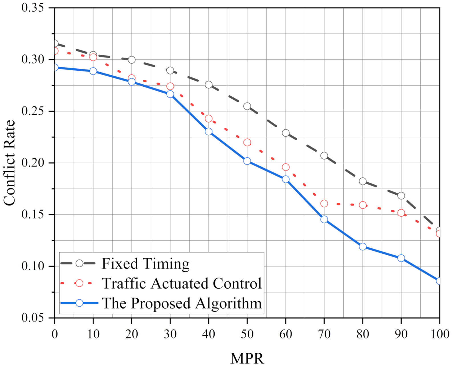
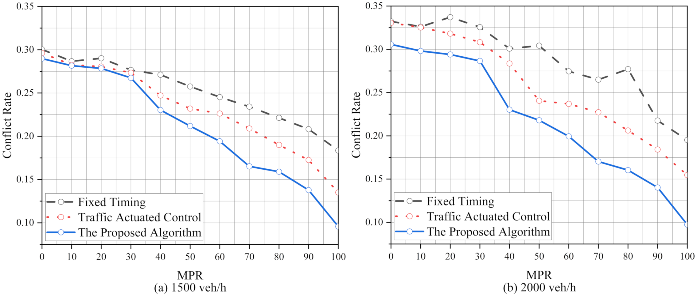
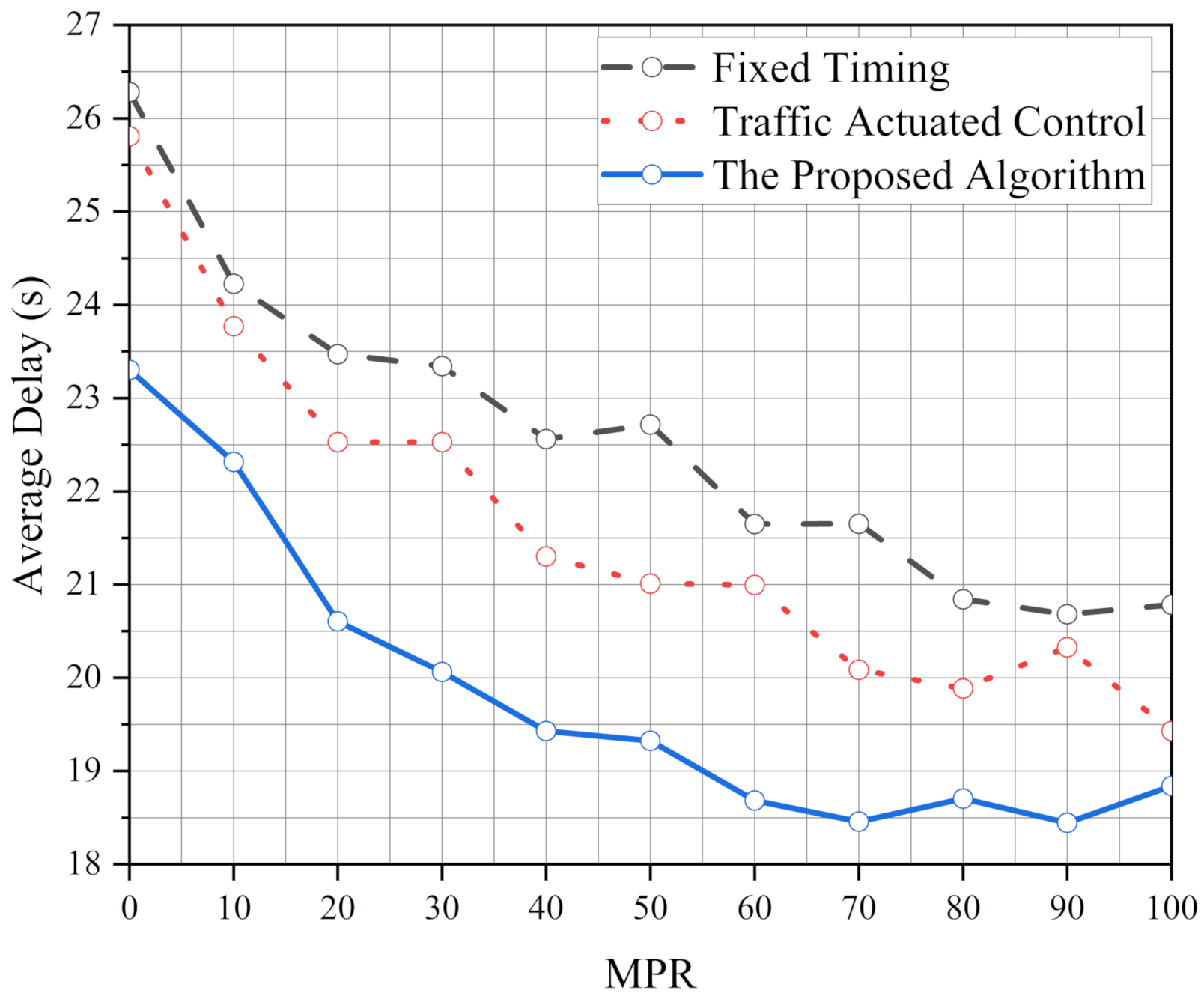
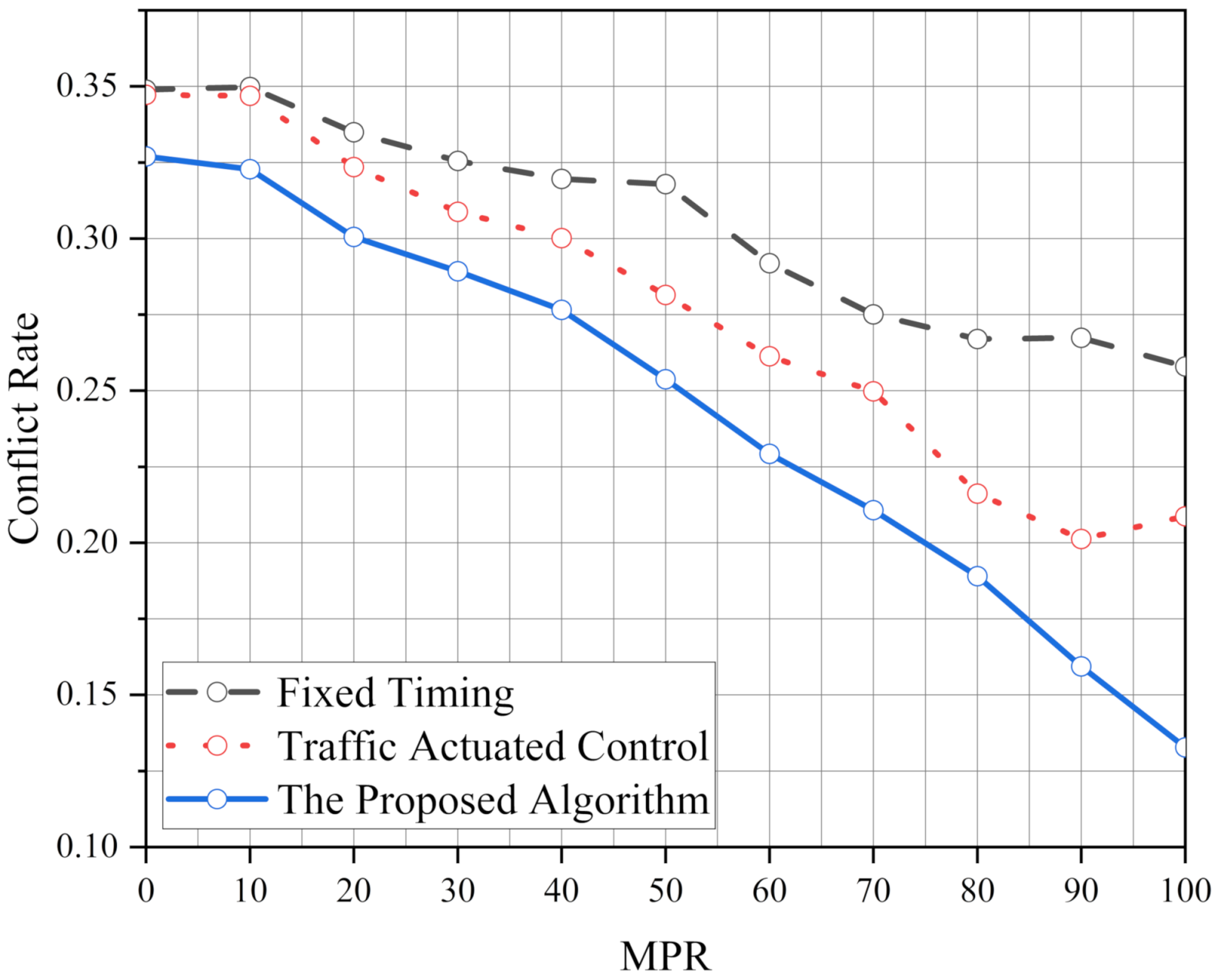
We proposed an ATSC based on the Q-learning algorithm to optimize the operational and safety performance of the intersection. The proposed algorithm has significant benefits for traffic control systems at isolated intersections. In addition, to meet the operational and safety performance of standard traffic demand, the robustness of the proposed algorithm is analyzed. The results show that the robustness of the proposed algorithm is better than FT and TAC. We also test the performance of the proposed algorithm in various traffic demands per approach (1000 veh/h, 1500 veh/h and 2000 veh/h) and its optimization ability increases with the increase in the traffic pressure. Moreover, it also shows excellent performance in an unbalanced traffic flow environment. After simulating, we find the operational and safety performance of our algorithm is more stable than FT and TAC. Finally, the effect of the intersection geometry is considered to verify the implementation of the proposed algorithm. It is found that the performance of the proposed algorithm is better than FT and TAC, and the ability of the proposed algorithm has been brought into full play under high MPRs.
The algorithm provides a new idea for the intelligent control of isolated intersections under the condition of mixed traffic flow. It also provides a research basis for collaborative control of multiple intersections.

Author Contributions

Conceptualization, Z.W. and S.W.; methodology, Z.W. and T.P.; software, T.P.; validation, Z.W., T.P. and S.W.; formal analysis, Z.W.; investigation, S.W.; resources, T.P.; data curation, T.P.; writing—original draft preparation, Z.W. and S.W.; writing—review and editing, T.P.; visualization, S.W.; supervision, T.P.; project administration, T.P. All authors have read and agreed to the published version of the manuscript.

Funding

This research received no external funding.

Institutional Review Board Statement

Not applicable.

Informed Consent Statement

Not applicable.

Data Availability Statement

Not applicable.

Acknowledgments

The authors would like to thank the medical staff fighting on the front line to combat the epidemic in Harbin, Heilongjiang Province.

Conflicts of Interest

The authors declare no conflict of interest.

Abbreviations

The following abbreviations are used in this manuscript:
ATSCAdaptive traffic signal control
HDVHuman-driving vehicle
CAVConnected and automated vehicle
IDMIntelligent driver model
CACCCooperative adaptive cruise control
MPRMarket penetration rate
FTFixed timing
TACTraffic actuated control
SUMOSimulation of urban mobility
TTCTime-to-collision

References

  1. Zhu, S.; Guo, K.; Guo, Y.; Tao, H.; Shi, Q. An adaptive signal control method with optimal detector locations. Sustainability 2019, 11, 727. [Google Scholar] [CrossRef] [Green Version]
  2. Lian, F.; Chen, B.; Zhang, K.; Miao, L.; Wu, J.; Luan, S. Adaptive traffic signal control algorithms based on probe vehicle data. J. Intell. Transp. Syst. 2021, 25, 41–57. [Google Scholar] [CrossRef]
  3. Chen, X.; Lu, J.; Zhao, J.; Qu, Z.; Yang, Y.; Xian, J. Traffic flow prediction at varied time scales via ensemble empirical mode decomposition and artificial neural network. Sustainability 2020, 12, 3678. [Google Scholar] [CrossRef]
  4. Al-Turki, M.; Ratrout, N.T.; Rahman, S.M.; Reza, I. Impacts of Autonomous Vehicles on Traffic Flow Characteristics under Mixed Traffic Environment: Future Perspectives. Sustainability 2021, 13, 11052. [Google Scholar] [CrossRef]
  5. Li, S.; Shu, K.; Chen, C.; Cao, D. Planning and Decision-making for Connected Autonomous Vehicles at Road Intersections: A Review. Chin. J. Mech. Eng. 2021, 34, 133. [Google Scholar] [CrossRef]
  6. Guo, Q.; Li, L.; Ban, X.J. Urban traffic signal control with connected and automated vehicles: A survey. Transp. Res. Part C Emerg. Technol. 2019, 101, 313–334. [Google Scholar] [CrossRef]
  7. Kuutti, S.; Fallah, S.; Katsaros, K.; Dianati, M.; Mccullough, F.; Mouzakitis, A. A survey of the state-of-the-art localization techniques and their potentials for autonomous vehicle applications. IEEE Internet Things J. 2018, 5, 829–846. [Google Scholar] [CrossRef]
  8. Tajalli, M.; Mehrabipour, M.; Hajbabaie, A. Network-level coordinated speed optimization and traffic light control for connected and automated vehicles. IEEE Trans. Intell. Transp. Syst. 2020, 22, 6748–6759. [Google Scholar] [CrossRef]
  9. Xu, B.; Ban, X.J.; Bian, Y.; Li, W.; Wang, J.; Li, S.E.; Li, K. Cooperative method of traffic signal optimization and speed control of connected vehicles at isolated intersections. IEEE Trans. Intell. Transp. Syst. 2018, 20, 1390–1403. [Google Scholar] [CrossRef]
  10. Gutesa, S.; Lee, J.; Besenski, D. Development and evaluation of cooperative intersection management algorithm under connected and automated vehicles environment. Transp. Res. Rec. 2021, 2675, 94–104. [Google Scholar] [CrossRef]
  11. Yang, K.; Guler, S.I.; Menendez, M. Isolated intersection control for various levels of vehicle technology: Conventional, connected, and automated vehicles. Transp. Res. Part C Emerg. Technol. 2016, 72, 109–129. [Google Scholar] [CrossRef]
  12. Wang, Y.; Yang, X.; Liang, H.; Liu, Y. A review of the self-adaptive traffic signal control system based on future traffic environment. J. Adv. Transp. 2018, 2018, 1096123. [Google Scholar] [CrossRef]
  13. Genders, W.; Razavi, S. Asynchronous n-step Q-learning adaptive traffic signal control. J. Intell. Transp. Syst. 2019, 23, 319–331. [Google Scholar] [CrossRef]
  14. Wang, H.; Yuan, Y.; Yang, X.T.; Zhao, T.; Liu, Y. Deep Q learning-based traffic signal control algorithms: Model development and evaluation with field data. J. Intell. Transp. Syst. 2021, 1–21. [Google Scholar] [CrossRef]
  15. Chu, T.; Wang, J.; Codecà, L.; Li, Z. Multi-agent deep reinforcement learning for large-scale traffic signal control. IEEE Trans. Intell. Transp. Syst. 2019, 21, 1086–1095. [Google Scholar] [CrossRef] [Green Version]
  16. Guo, J.; Harmati, I. Evaluating semi-cooperative Nash/Stackelberg Q-learning for traffic routes plan in a single intersection. Control Eng. Pract. 2020, 102, 104525. [Google Scholar] [CrossRef]
  17. Abdoos, M.; Mozayani, N.; Bazzan, A.L. Hierarchical control of traffic signals using Q-learning with tile coding. Appl. Intell. 2014, 40, 201–213. [Google Scholar] [CrossRef]
  18. Wang, X.; Ke, L.; Qiao, Z.; Chai, X. Large-scale traffic signal control using a novel multiagent reinforcement learning. IEEE Trans. Cybern. 2020, 51, 174–187. [Google Scholar] [CrossRef]
  19. Essa, M.; Sayed, T. Self-learning adaptive traffic signal control for real-time safety optimization. Accid. Anal. Prev. 2020, 146, 105713. [Google Scholar] [CrossRef]
  20. Abdoos, M. A Cooperative Multiagent System for Traffic Signal Control Using Game Theory and Reinforcement Learning. IEEE Intell. Transp. Syst. Mag. 2020, 13, 6–16. [Google Scholar] [CrossRef]
  21. Wang, L.; Li, H.; Guo, M.; Chen, Y. The Effects of Dynamic Complexity on Drivers’ Secondary Task Scanning Behavior under a Car-Following Scenario. Int. J. Environ. Res. Public Health 2022, 19, 1881. [Google Scholar] [CrossRef] [PubMed]
  22. Wang, L.; Li, H.; Li, S.; Bie, Y. Gradient illumination scheme design at the highway intersection entrance considering driver’s light adaption. Traffic Inj. Prev. 2022, 1–5. [Google Scholar] [CrossRef] [PubMed]
  23. Olayode, I.O.; Tartibu, L.K.; Okwu, M.O.; Severino, A. Comparative Traffic Flow Prediction of a Heuristic ANN Model and a Hybrid ANN-PSO Model in the Traffic Flow Modelling of Vehicles at a Four-Way Signalized Road Intersection. Sustainability 2021, 13, 10704. [Google Scholar] [CrossRef]
  24. Chen, K.; Zhao, J.; Knoop, V.L.; Gao, X. Robust signal control of exit lanes for left-turn intersections with the consideration of traffic fluctuation. IEEE Access 2020, 8, 42071–42081. [Google Scholar] [CrossRef]
  25. Chiou, S.W. A robust signal control system for equilibrium flow under uncertain travel demand and traffic delay. Automatica 2018, 96, 240–252. [Google Scholar] [CrossRef]
  26. Tobita, K.; Nagatani, T. Green-wave control of an unbalanced two-route traffic system with signals. Phys. A Stat. Mech. Its Appl. 2013, 392, 5422–5430. [Google Scholar] [CrossRef]
  27. Zhu, L.; Jia, B.; Yang, D.; Wu, Y.; Yang, G.; Gu, J.; Qiu, H.; Guo, Q. Modeling the traffic flow of the urban signalized intersection with a straddling work zone. J. Adv. Transp. 2020, 2020, 1496756. [Google Scholar] [CrossRef]
  28. Arvin, R.; Kamrani, M.; Khattak, A.J. The role of pre-crash driving instability in contributing to crash intensity using naturalistic driving data. Accid. Anal. Prev. 2019, 132, 105226. [Google Scholar] [CrossRef]
  29. Rahman, M.S.; Abdel-Aty, M.; Lee, J.; Rahman, M.H. Safety benefits of arterials’ crash risk under connected and automated vehicles. Transp. Res. Part C Emerg. Technol. 2019, 100, 354–371. [Google Scholar] [CrossRef]
  30. TRB. Highway Capacity Manual 2010; Transportation Research Board, National Research Council: Washington, DC, USA, 2010; Volume 1207. [Google Scholar]
  31. Lopez, P.A.; Behrisch, M.; Bieker-Walz, L.; Erdmann, J.; Flötteröd, Y.P.; Hilbrich, R.; Lücken, L.; Rummel, J.; Wagner, P.; Wießner, E. Microscopic traffic simulation using sumo. In Proceedings of the 2018 21st International Conference on Intelligent Transportation Systems (ITSC), Maui, HI, USA, 4–7 November 2018; pp. 2575–2582. [Google Scholar]
  32. Mousavi, S.M.; Osman, O.A.; Lord, D.; Dixon, K.K.; Dadashova, B. Investigating the safety and operational benefits of mixed traffic environments with different automated vehicle market penetration rates in the proximity of a driveway on an urban arterial. Accid. Anal. Prev. 2021, 152, 105982. [Google Scholar] [CrossRef]
Figure 1. The flow of the proposed algorithm.
Sustainability 14 05751 g001
Figure 2. The intersection builds in SUMO.
Sustainability 14 05751 g002
Figure 3. The average delay under various MPRs using the proposed algorithm, FT and TAC in 1000 veh/h.
Sustainability 14 05751 g003
Figure 4. The conflict rate under various MPRs using the proposed algorithm, FT and TAC in 1000 veh/h.
Sustainability 14 05751 g004
Figure 5. The average delay under various MPRs using the proposed algorithm, FT and TAC in 1500 veh/h and 2000 veh/h.
Sustainability 14 05751 g005
Figure 6. The conflict rate under various MPRs using the proposed algorithm, FT and TAC in 1500 veh/h and 2000 veh/h.
Sustainability 14 05751 g006
Figure 7. The average delay under various MPRs using the proposed algorithm, FT and TAC in unbalanced flow.
Sustainability 14 05751 g007
Figure 8. The conflict rate under various MPRs using the proposed algorithm, FT and TAC in unbalanced flow.
Sustainability 14 05751 g008
Figure 9. The irregular intersection builds in SUMO.
Sustainability 14 05751 g009
Figure 10. The average delay under various MPRs using the proposed algorithm, FT and TAC at the irregular intersection.
Sustainability 14 05751 g010
Figure 11. The conflict rate under various MPRs using the proposed algorithm, FT and TAC at the irregular intersection.
Sustainability 14 05751 g011
Table 1. The state set for the proposed algorithm.
StateLink OrderStateLink Order
S 1 q 1 q 2 q 3 q 4 S 13 q 2 q 3 q 1 q 4
S 2 q 1 q 2 q 4 q 3 S 14 q 2 q 4 q 1 q 3
S 3 q 1 q 3 q 2 q 4 S 15 q 3 q 2 q 1 q 4
S 4 q 1 q 4 q 2 q 3 S 16 q 4 q 2 q 1 q 3
S 5 q 1 q 3 q 4 q 2 S 17 q 3 q 4 q 1 q 2
S 6 q 1 q 4 q 3 q 2 S 18 q 4 q 3 q 1 q 2
S 7 q 2 q 1 q 3 q 4 S 19 q 2 q 3 q 4 q 1
S 8 q 2 q 1 q 4 q 3 S 20 q 2 q 4 q 3 q 1
S 9 q 3 q 1 q 2 q 4 S 21 q 3 q 2 q 4 q 1
S 10 q 4 q 1 q 2 q 3 S 22 q 4 q 2 q 3 q 1
S 11 q 3 q 1 q 4 q 2 S 23 q 3 q 4 q 2 q 1
S 12 q 4 q 1 q 3 q 2 S 24 q 4 q 3 q 2 q 1
Table 2. The differences in the average delay under various MPRs using the proposed algorithm compared with FT and TAC in 1000 veh/h.
MPR010%20%30%40%50%60%70%80%90%100%
FT 11.44 % 11.42 % 9.18 % 9.94 % 16.95 % 17.05 % −14.73% 14.54 % −15.44% 16.83 % 15.46 %
TAC 9.73 % 5.23 % −1.00%1.32%1.08% 0.50 % 5.56 % 3.69 % −7.59% 7.77 % 9.31 %
Table 3. The differences in the conflict rate under various MPRs using the proposed algorithm compared with FT and TAC in 1000 veh/h.
MPR010%20%30%40%50%60%70%80%90%100%
FT−7.35%−5.16%−7.11%−7.88%−16.45%−20.81% 19.56 % −29.82%−34.69%−35.97%−36.34%
TAC−5.16%−4.43%−1.23%−2.74%−5.15%−8.22%−5.99%−9.57%−25.25%−28.95%−34.82%
Table 4. The differences in the average delay under various MPRs using the proposed algorithm compared with FT and TAC in robust analysis.
Traffic Demand (veh/h)MPR010%20%30%40%50%60%70%80%90%100%
1500FT−25.23%−21.27%−24.70%−28.97%−24.91%−24.48%−23.29%−21.09%−24.45%−19.94%−23.70%
TAC−17.82%−15.17%−15.70%−23.24%−6.33%−9.46%−10.30%−8.81%−11.96%−5.26%−6.46%
2000FT−25.24%−25.21%−23.89%−27.58%−28.35%−31.92%−27.98%−29.13%−28.10%−25.15%−26.28%
TAC−11.05%−9.24%-8.53%−13.43%−4.54%−10.39%−8.28%−11.17%−9.77%−9.08%−11.57%
Table 5. The differences in the conflict rate under various MPRs using the proposed algorithm compared with FT and TAC in robust analysis.
Traffic Demand (veh/h)MPR010%20%30%40%50%60%70%80%90%100%
1500FT−3.51%−1.76%−4.05%−3.28%−15.02%−17.74%−20.80%−29.42%−28.15%−33.81%−47.84%
TAC−2.16%−0.31%−0.74%−2.15%−6.77%−8.68%−14.16%−20.90%−16.29%−20.14%−29.13%
2000FT−8.01%−8.60%−12.78%−12.00%−23.47%−28.33%−27.38%−35.73%−42.13%−35.54%−50.12%
TAC−7.53%−8.36%−7.57%−7.01%−18.83%−9.36%−15.83%−25.07%−22.23%−23.88%−37.04%
Table 6. The differences in the average delay under various MPRs using the proposed algorithm compared with FT and TAC in unbalanced flow.
MPR010%20%30%40%50%60%70%80%90%100%
FT−29.55%−30.06%−32.12%−28.68%−29.08%−31.35%−28.82%−25.35%−24.83%−27.40%−24.28%
TAC−28.04%−27.09%−30.06%−27.02%−22.07%−23.46%−18.85%−16.74%−17.54%−18.85%−17.06%
Table 7. The differences in the conflict rate under various MPRs using the proposed algorithm compared with FT and TAC in unbalanced flow.
MPR010%20%30%40%50%60%70%80%90%100%
FT−23.93%−23.67%−24.46%−23.02%−26.24%−27.24%−31.48%−30.65%−28.78%−36.92%−44.80%
TAC−20.32%−19.02%−21.90%−19.80%−10.39%−13.33%−9.47%−8.16%−3.24%−9.58%−19.52%
Table 8. The differences in the average delay under various MPRs using the proposed algorithm compared with FT and TAC at the irregular intersection.
MPR010%20%30%40%50%60%70%80%90%100%
FT−11.34%−7.89%−12.22%−14.05%−13.89%−14.93%−13.70%−14.74%−10.26%−10.81%−9.36%
TAC−9.71%−6.12%−8.54%−10.95%−8.79%−8.02%−11.00%−8.10%−5.93%−9.26%−3.04%
Table 9. The differences in the conflict rate under various MPRs using the proposed algorithm compared with FT and TAC at irregular intersection.
MPR010%20%30%40%50%60%70%80%90%100%
FT−6.27%−7.73%−10.26%−11.13%−13.48%−20.17%−21.45%−23.37%−29.20%−40.38%−48.53%
TAC−5.82%−6.97%−7.09%−6.33%−7.87%−9.82%−12.25%−15.64%−12.54%−20.79%−36.38%
Publisher’s Note: MDPI stays neutral with regard to jurisdictional claims in published maps and institutional affiliations.

