Statistical Study Based on the Kriging Method and Geographic Mapping in Rigid Pavement Defects in Southern Chile

Abstract

ASTM D6433 is used to assess the need for maintenance of pavement sections. Although the Pavement Condition Index (PCI) factor calculation method provides reliable values, this method analyzes sections and defects individually and indicates current maintenance needs, but it cannot be used to predict the occurrence of new defects. Therefore, it is necessary to complement this method by considering variables that influence the occurrence of faults, among which are the geospatial distribution and the specific characteristics of the slabs. This research focuses on the identification of multiple types of disturbances that exist in Portland Cement Pavements (PCC), located in a high traffic area in the city of Valdivia (Chile). A spatial geostatistical relationship is established through visual inspection using geographical maps, as well as distribution, using the kriging method. This technique makes use of variograms that allow quantifying the parameters used in this study, thus expressing the spatial autocorrelation of the faults analyzed. From the results obtained by spatial geostatistics and kriging, it is possible to generate a data correlation for the distribution and characteristics of the streets considered. In addition, a co-kriging method is established instead of an ordinary kriging method. The relationship between observed and predicted values improved from 0.3327 to 0.5770. The width of the slabs, as well as some streets, is shown in our analysis to be unimportant. For better model accuracy, the number of covariates associated with the type of vehicle traffic, the age and shape of the slabs, and the construction techniques used for the pavement needs to increase.

1. Introduction

Today, roads have gone from being rudimentary paths to modern streets and highways, conceived not only for foot traffic but also for motor vehicle transportation on a large scale [1,2]. The distresses present in highways, roads, and streets are directly related to the comfort and security of the users, who could be subjected to a traffic accident at any moment [3,4]. Consequently, there is a need to identify the distresses caused by the different parameters affecting roadways, with the goal of getting to the core of the problem and find a solution [5]. To this effect, relying on a method of evaluating the state of the pavement and the distresses presented therein is indispensable to an efficient identification of mitigation measures [6]. To carry out this analysis, according to the Pavement Condition Index (PCI) method indicated in the ASTM D6433-18 [7], visual inspections and measurements of distresses are made on the existing pavements, both flexible and rigid, generating a factor through which the priorities of action are established according to the severity of the damages observed in the different sections of the analyzed areas. The main values measured are related to the length, width, and depth of the crack or deterioration. However, the analysis carried out evaluates these zones individually, without considering the defects of nearby areas or the relationship between the types of defects and their distribution, to more accurately predict the future appearance of new damages in the same zone or nearby areas.

Gubler et al. published a study, focused on the analysis of the main urban roads in the USA, to find a strategy that could minimize the accumulated damage of the roads, since 28% of the pavements are in poor or deficient condition [8]. The unintended consequence of this decision for road users was an increased maintenance cost of their vehicles and the increased risk of traffic accidents. Roads in critical condition represent 53% of the total distance driven annually in the USA, making the evaluation of the dimensions of these pavement distresses paramount. The organization that carried out this study—TRIP—promotes transport policies that aid in alleviating traffic congestion and its impact on air quality, improving the conditions of roadway infrastructure, building safer roads, and bettering economic productivity [9].

The current situation in Chile is not very different from that in the USA. Chile has an approximate road network of 82,133.78 km, of which 40% is paved. However, the quality of the Portland Cement Concrete (PCC) pavement is not always adequate, due to the lack of maintenance and inspection and, in some cases, poor techniques used in construction [9]. Valdivia is a city located in the Chilean South macro-zone, where it is common to find pavements in poor condition, with potholes and cracks, especially in the city center, where there is a greater volume of traffic. It is important to identify the areas where the most distresses concentrate and to link their origin with local characteristics, thus seeking a mathematical relationship with the distresses in the adjacent slabs to predict their distribution and nature [10]. In so doing, preventive measures could be taken in a timely fashion, at the least minimizing the damages and extending the life of the pavements [11].

Other types of studies focusing on the optimization of the geometry of the slab have been carried out to reduce the thickness of the slab, minimize the devices of the mechanical transfer, and minimize the damage produced. In a theoretical study, Roesler, Cervantes, and Amirkhanian showed, through academic research, that a thinner size reduces load and induced tensile stresses, for large-scale testing [12].

In 2013, a study was published focusing on the revision of the methods used for predicting the performance of pavements (rigid and flexible), searching for solutions prior to breakage. Simulations were made from the data obtained on the pavement built on Route 50 in Ohio (USA). It was determined that the long-term performance of a pavement can be calculated from a small fraction of its design life and a set of purely statistical/empirical algorithms. However, the research mentions that the test pavement fails due to transverse cracking, and the progression of the crack does not depend on the type of sealing treatment used [13].

A more recent study has also used Bayesian modeling to identify the most influential variables and to quantify the uncertainty of linear regression models predicting the occurrence of deformation in flexible pavement structures [14]. It was possible to establish the variables with the most significant variability and those with the greatest uncertainty by using the best models developed in conjunction with the Bayesian technique. Therefore, the Bayesian model could also be used for rigid pavements when detailed information is available on the properties and conditions of the rigid pavements to be analyzed.

Urban road pavements can be classified through high-resolution spatial images, thus seeking options to help solve the progressive deterioration caused by increased vehicle traffic. Majore et al. conducted a study based on the use of orthoimages generated by geographical institutes with the intention of mapping roads in the Czech Republic that needed restoration. Characterization was done by observing the orthoimages and creating “interpretation keys” related to the class or type of road and its characteristics. The result provided the resources to supply, quickly and accurately, information on roads in poor condition [15].

As can be seen from the analysis of the state of the art, ASTM D6433 is used to assess the need for maintenance of pavement sections. Although the PCI factor calculation method provides reliable values, this method analyzes sections and defects individually and indicates current maintenance needs, but it cannot be used to predict the occurrence of new defects.

This research helps to simplify the analysis of pavement defects in large areas, where automated means are not available. The analysis focuses on identifying the main types of distresses present in the PCC pavements in the center of Valdivia (Chile) and the relation between them, using the Instructive for visual inspection of paved roads (National Directorate of Roads of Chile 2013), based on AASHTO-93 [16] and ASTM D6433-18 [7], and considering the characteristics and dimensions of the slabs and their distresses. The autocorrelation of defects will be estimated through kriging analysis, allowing for the interpolation of distresses beyond the sample slabs; in turn, this procedure will help analyze the relationship between the faults observed in different sections and estimate the best way to develop successive construction and repair processes of pavements.

The method used allows to establish the relationship in the occurrence of pavement defects from the geospatial distribution of the streets and, at the same time, adds variables specific to each of the streets.

2. Materials and Methods

A geographical information system (GIS) consists of an organized integration of hardware, software, and geographical data, designed to input, administer, manipulate, analyze, model, and plot data (results output) or spatially referenced objects [17,18]. A GIS is a computerized system capable of maintaining and using data with exact locations on the earth’s surface, representing real objects (roads, land use, altitudes, etc.) digitally in two types of formats: (1) raster or cellular, a model centered more on space properties than on location precision, and identified by the characteristic size of the cells that make up the mesh; the larger they are, the smaller the representation of the geographical space; and (2) vector, a model focused on the precision of location of elements over space, where the objects to be represented have defined limits [6,19,20].

2.1. Kriging

Kriging models are specially developed for spatial analysis. The error term is spatially autocorrelated, while independent in linear models. Caballero et al. explained that kriging is an interpolation method by which the best linear unbiased estimations of point values can be obtained, which permits the selection of the weighted average of the values of the samples that have minimal variance [21]. Hernandez et al. employed the kriging method to predict the average annual daily traffic on the road network of the Basque Autonomous Community and concluded that kriging interpolation methods area adequate to perform this type of analysis [22]. Supposing that information is known about a certain attribute Z in different positions of a domain D, the objective would be trying to predict the value of Z in a place where the data is not registered, considering the covariance structure of the random variables Z(s) defined in those places where measurements were registered [23]. The method employed is similar to a multiple linear regression applied in a spatial context, where the random variables Z(S) play the role of regressive variables, and the random variable at the point of interest “Z(S₀)” acts as a dependent variable. The precision depends upon a variety of factors, such as: (1) the number of samples and the quality of the information at each point; (2) the distance between the samples and the point to be assessed; and (3) the spatial continuity in consideration [21].

The kriging predictor depends on the model used for the random function Z(s). Generally, Z(s) is broken down into one trend component m(s) and one residual component ε(s), as expressed by the equation Equation (1):

$$Z\left(s\right)=m\left(s\right)+ϵ\left(s\right),$$

(1)

where the variogram or the covariogram of ε(s) is presumed to be known.

The expected value of Z in the s position represents the value of the trend in said position Equation (2):

$$E\left[Z\left(s\right)\right]=m\left(s\right).$$

(2)

In this article, the analysis begins with the ordinary kriging method. It proposes that the value of the variable of the unmeasured site can be estimated as a linear combination of the random variables using Equation (3):

$$Z^{*}\left(s_0\right)={\displaystyle \sum }_{i=1}^n{\lambda }_{i}Z\left(s_i\right),$$

(3)

where λ_i represents the weightings of the values of the variables in the sampled sites. They are calculated as a function of the distance between the sampled points and the point where the corresponding prediction will be conducted. Z*(S₀) is the best linear unbiased predictor obtained in such a way as to minimize the variance of the prediction error, subject to the sum of the weightings of values equaling one:

$$V\left(Z^{*}{}_{\left(s_0\right) }-Z_{\left(s_0\right)}\right), subject to {\displaystyle \sum }_{i=1}^n{\lambda }_i=1.$$

(4)

Moreover, the application of the Lagrange multipliers method [24] to solve Equation (4), in conjunction with the determination of the covariance matrix from the spatial autocorrelation structure, allows for the determination of the optimal λ_i weighting values.

The co-kriging method will also be employed; it uses j covariates in the ordinary kriging method to obtain a better estimator:

$$Z^{*}\left(s_0\right)={\displaystyle \sum }_{j=1}^m{\displaystyle \sum }_{i=1}^n{\lambda }_{j,i}{Z}_j\left(s_i\right).$$

(5)

2.2. Variogram

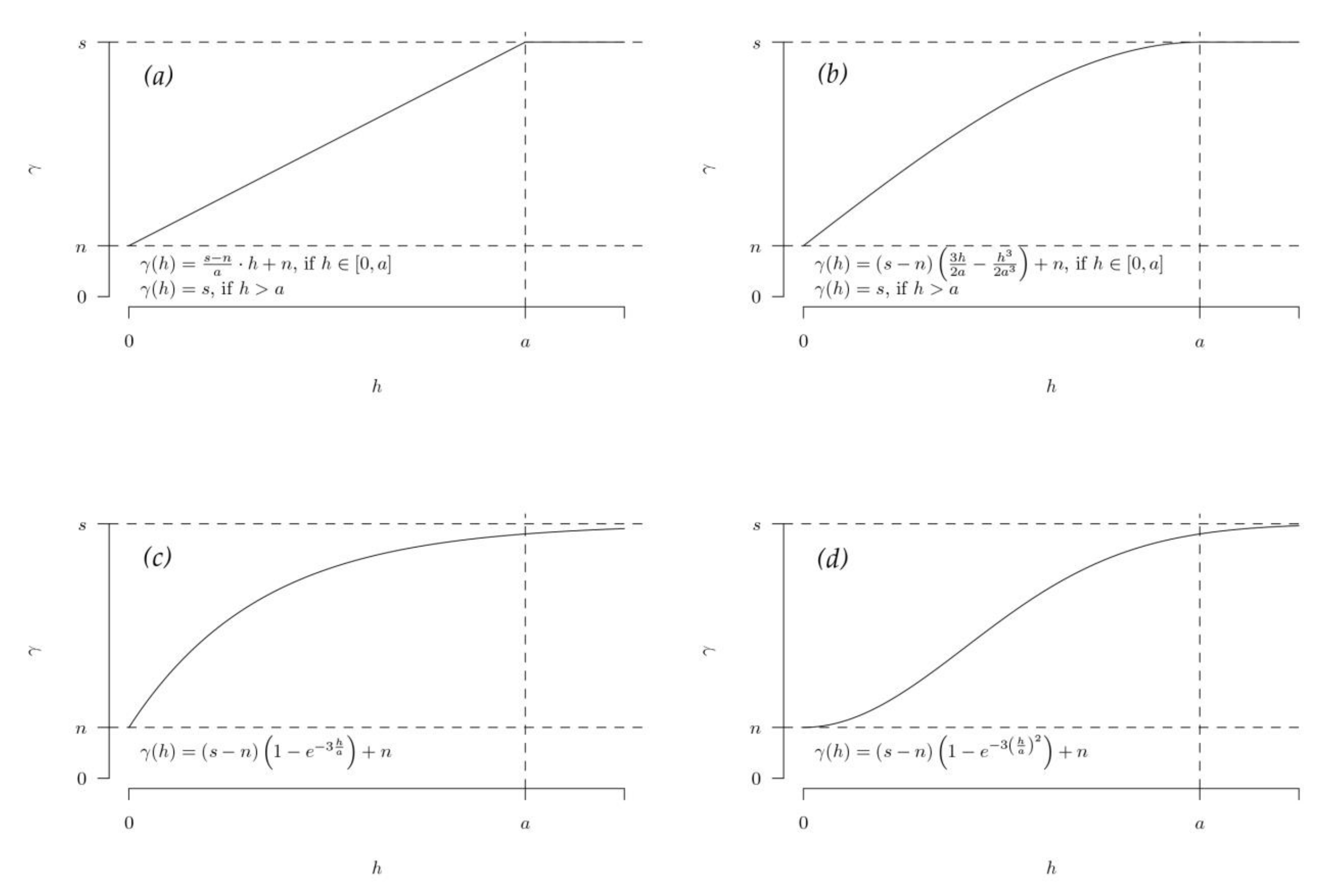
The variogram is an essential geostatistical tool that expresses the spatial correlation between sample values. Mathematically, it is defined as the average of the squares of differences between pairs of samples, separated by a distance h [25]. The spatial continuity is reflected in the growth rate of the variance following the distance from the sample [26]. The kriging method usually uses four types of variograms, as shown in Figure 1: (1) linear; (2) spherical; (3) exponential; and (4) Gaussian [27].

2.3. Data Collection and Registration

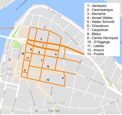
This study was carried out in the center of Valdivia (Chile), since it is the sector with the highest concentration of traffic. The concrete slabs analyzed correspond to the area between the intersections of Janequeo–O’Higgins, O’Higgins–Arauco, Arauco–Walter Schmidt, and Walter Schmidt–Carampangue streets (Figure 2).

A visual registration of the distresses in the slabs was carried out. The slabs were examined 10 m from the initial reference point and, subsequently, every 20 m, to evaluate the intermediate points. Upon reaching each measurement point, a mark was made to have a reference and track the required distance from the reference point. Subsequently, the dimensions of each slab (length and width) were measured at three points to obtain an average value. The cracks were inspected and their characteristics recorded (length, width, and depth), to be drawn. Eight types of distresses were recorded; the first four corresponded to longitudinal, transversal, corner, and oblique cracks (Instructive for visual inspection of paved roads, 2013). However, four additional categories were incorporated, since distresses were found that did not correspond to the categories mentioned above: (1) incomplete longitudinal; (2) incomplete transversal; (3) incomplete corner; and (4) incomplete oblique.

The record is shown in

Table 1. Statistic summary of the dimensions of the slabs.

Statistics	Width (m)	Length (m)
Average	8.58	5.31
Std. Dev.	1.91	1.91
Minimum	4.67	1.79
Maximum	13.55	11.44

and is based on the record used by the Chilean Ministry of Housing and Urban Planning for the visual inspection of urban pavements.

• In this paper: Abs corresponds to the abscissa, the distance at which the slab located from the initial reference point.
• Concrete Slab N° is the number of each slab observed, in each street, the numbering restarted.
• Runway refers to whether the slab belongs to the left or right side runway; however, there was the case of runway that consisted of 3 and 4 concrete slabs per abscissa, and, in the case of the 3 concrete slabs, we marked the central concrete slab with the letter C, while, in the case of the 4 concrete slabs, they entered as CD (center-right) or CI (center-left), as appropriate.
• Size of the concrete slab refers to the width and length of the concrete slabs, for both the values, recorded in 3 points, given the irregularity in the geometry of the slabs, to then obtain an average. The unit of measurement used was meters.
• Type of failure denotes the name of the failure; it can be one of the eight previously described, then the dimensions of these, registering length, width, and depth of the failure. The range is measured in meters, while the other two are measured in millimetres.

Moreover, all the previously registered points were geo-referenced in degrees, minutes, and seconds (geographic coordinate system WGS84 zone 18s) [28].

3. Results

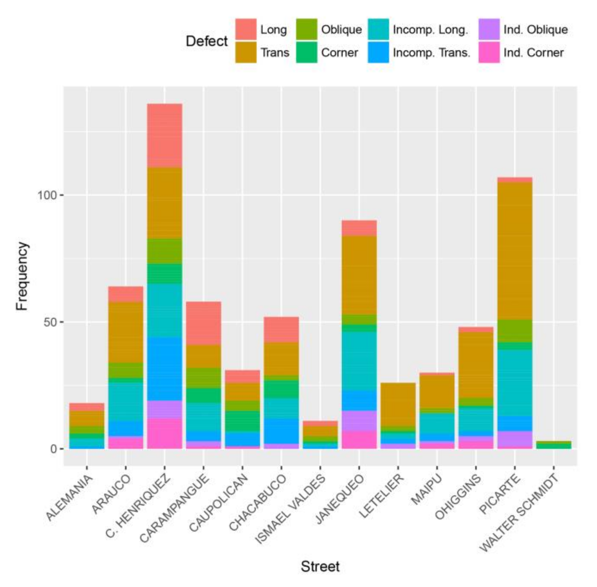
Figure 3 shows the distribution of defects per street. The streets with the most defects are Camilo Henríquez (136 in 500m, 20.18% of total defects) and Picarte (107 in 450m, 15.88% of total defects). The least compromised street was Walter Schmidt (3 defects in 251m, 0.45% of total defects). It is possible to observe that, while Camilo Henríquez street has a wide range of different defects in these streets, both Picarte and Janequeo streets have predominantly transverse and incomplete longitudinal defects. The most frequent defect type was transverse (34.42%), with incomplete longitudinal in second place (18.99%). Incomplete oblique and incomplete corner defects, the least frequent in our sample, accounted only for 4.59%, respectively. In relative terms, the streets with the highest number of defects per linear meter were Letelier (0.43) and Maipú (0.54). Only 60% of the detected defects could be cataloged using the Visual Inspection Instructions [29], which points to the necessary updating of this instrument.

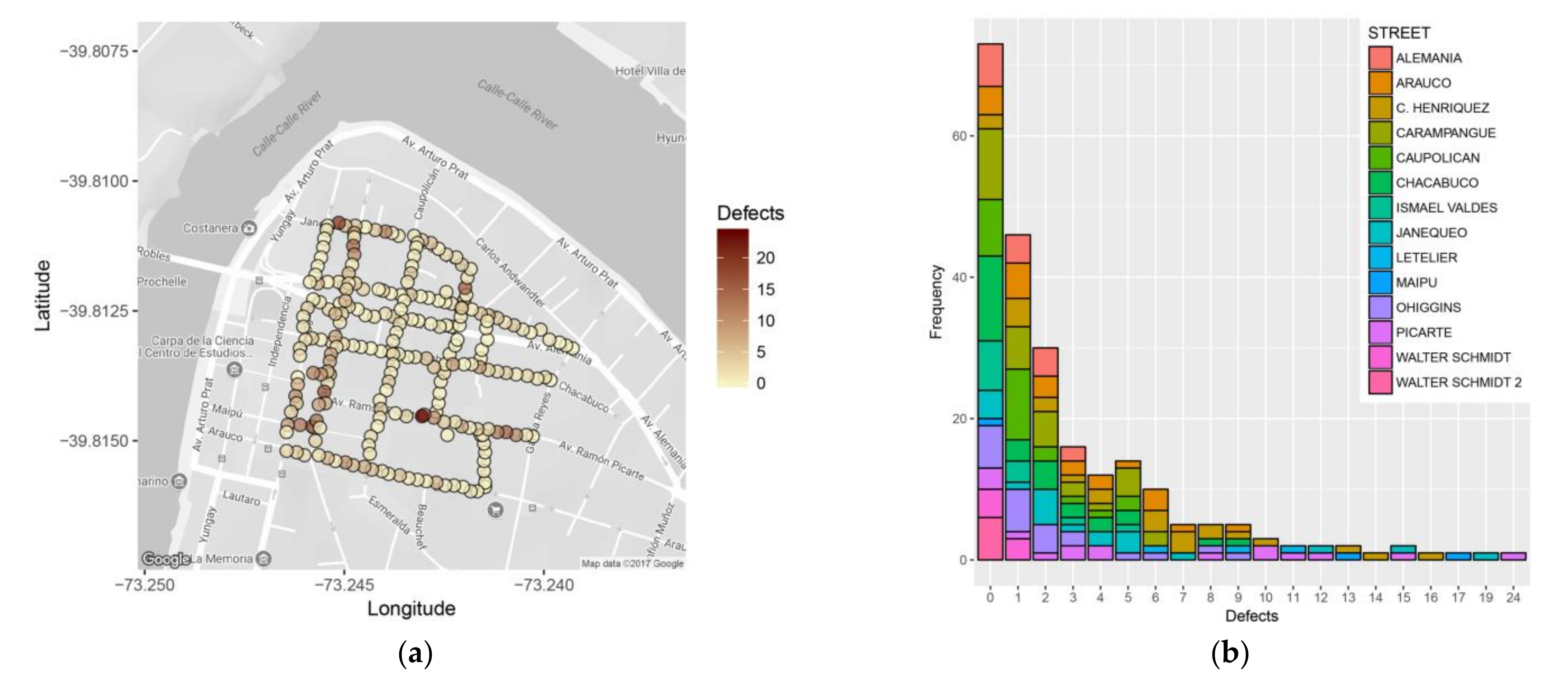
Figure 4a shows the number of defects at each sample point, while Figure 4b shows a histogram of the distribution of the number of points with a certain number of defects by street. The number of points with few or no defects is much greater than those with many defects. The sampling point with the highest number of defects (24) was found in Picarte street. The largest average of defects per point is reported in Maipú (10.00) and Letelier (8.67) streets, while the highest standard deviation is that of Maipú (8.88) and Janequeo (5.19) streets.

Although the city of Valdivia does not seem to follow a stable design regulation for slab construction, and the slabs in our sample are, on average, wider than than they are long (see

Table 2. Visual inspection of paved roads.

Abs	Concrete Slab	Runway		Size of the Concrete Slab								Type of Failure
				Length (m)				Breadth (m)				Name of the Failure	Dimensions of Failure (m)
	N°	Left	Right	L1	L2	L3	Lt	A1	A2	A3	At		L	Breadth	Depth
	1	x		4.9	4.8	6.2	5.53	8.6	8.4	8.6	8.5	transversal	1.03	8.67	5.58

), the standard deviation is the same in width as in length. Transverse defects are almost three times more frequent than longitudinal ones (232 versus 79), while almost twice as many slabs show transverse defects than longitudinal ones (94 versus 59). Skewness is more extreme for the length (1.03) than the width (0.67).

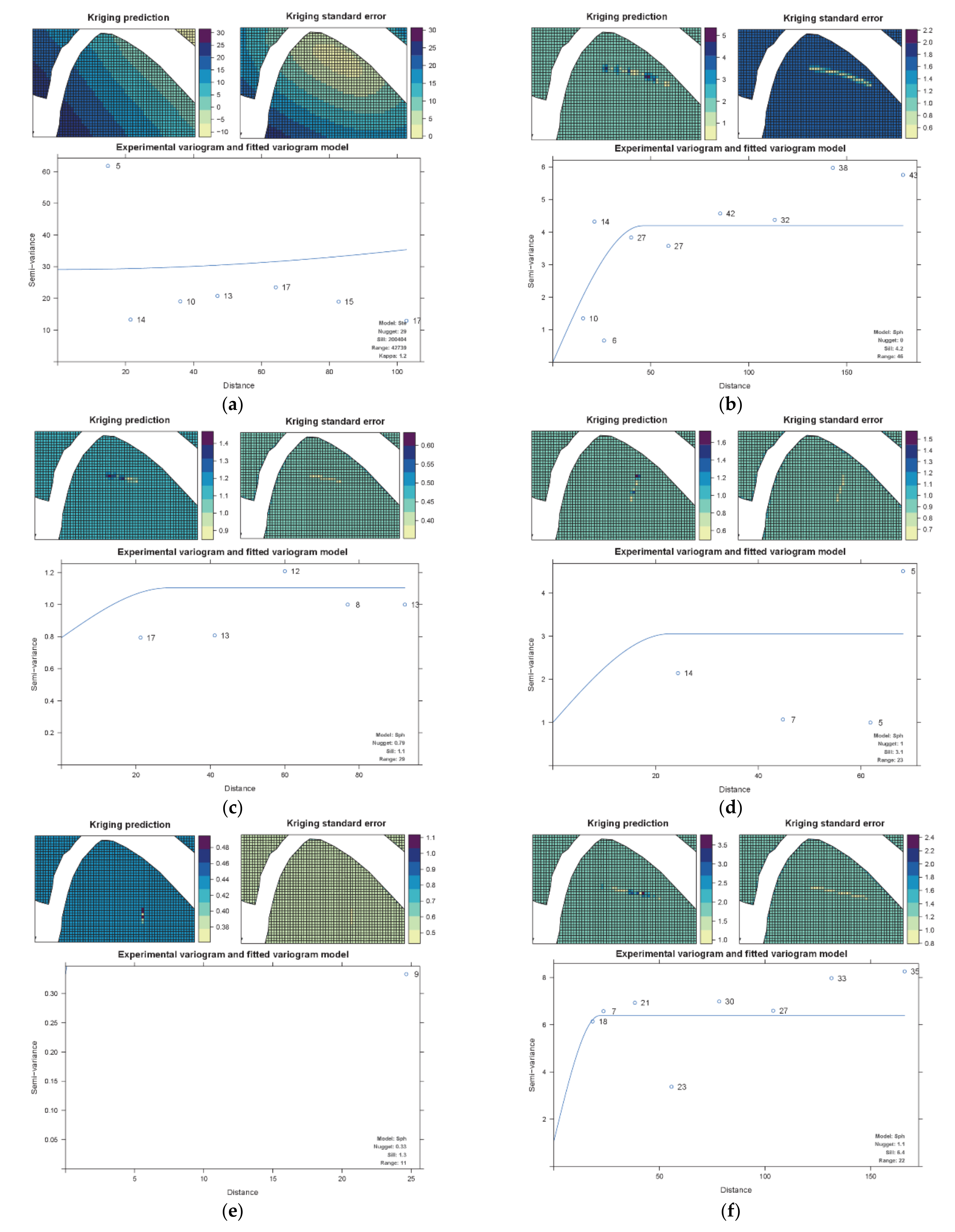
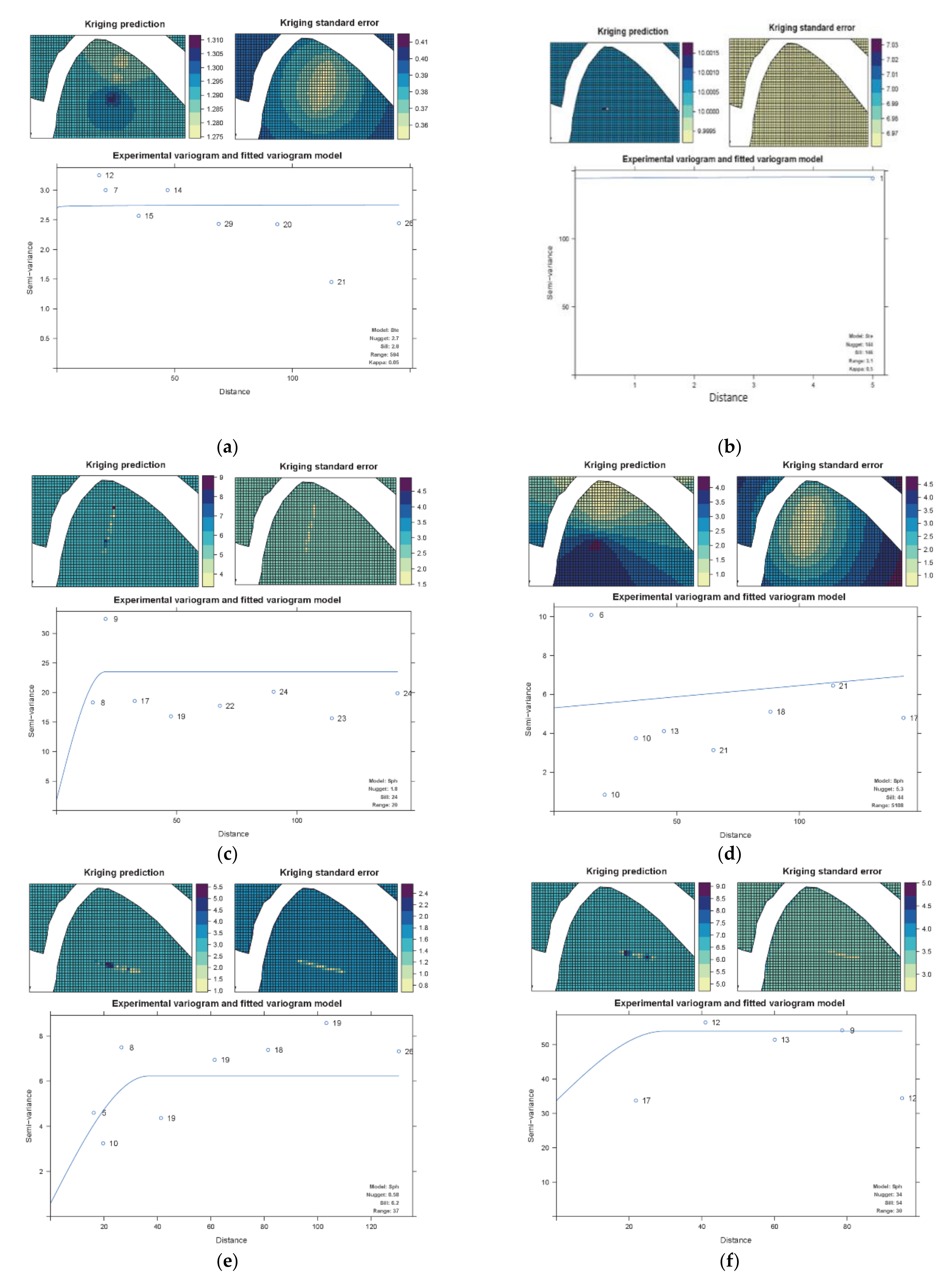
The pavement defect data of each street of the city center of Valdivia were modeled with an ordinary Kriging via the “autoKrige” function of GNU R’s “automap” package. This function automatically selects the best fitting from the variogram models shown in Figure 1. The results presented in Figure 5 and Figure 6 are separated into three plots per subfigure. First is the kriging prediction of the number of defects the model estimates in each grid point (40 rows by 60 columns). Given that a sample of slabs per street was gathered, the kriging method estimates the defects for the whole grid, i.e., for the sampled and non-sampled grid points. It is an interpolation with the variogram that best fits the data. The second plot is the standard error of the kriging prediction, i.e., the standard deviation of the sampling distribution. For most streets, it is possible to observe that the standard error is smaller in the grid points approximately belonging to the street than in those not. There is data for the former, not the latter. Hence, the predictability of defects decays with the distance to the street.

Nevertheless, the results of both the kriging prediction and its standard error show that the kriging model cannot make an adequate prediction in some streets, such as Janequeo (Figure 5a), O’Higgins (Figure 6d), and Caupolicán (Figure 6a). The prediction fails as there is no spatial autocorrelation in the defects of the streets. This result is expected for some streets as not all the variance is spatially explained. For example, some slabs might be replaced, or there are not enough data points for a good model fit. The algorithm in “autoKrige” still selects the “best” variogram for the street data, although it might not be a good one. Finally, the bottom plot is the variogram plot for the data points. This model is used to predict the defects in the prediction. The spherical model fits most streets better, which means that, while variance grows in a non-linear way, it does not have an asymptotic behavior. Nonetheless, it is possible to observe the lack of this asymptotic behavior in the streets where spatial autocorrelation is hard to identify. Table 2 Provides a statistic summary of the dimensions of the slabs.

Next, the possibility of evaluating the different variograms for a model that considers the entire area of the city studied was explored, employing the cross-validation method. Using the cross-validation method to evaluate the four variograms used by ordinary kriging, we observe in

Table 3. Model comparison using the cross-validation method.

	Linear	Spherical	Exponential	Gaussian
Correlation between Observed and predicted values	0.3128	0.3214	0.3327	0.1308
Correlation between Observed values and Residuals	−0.0075	0.018	0.0036	−0.0665
RMSE	3.7	3.689	3.6730	3.87

that the best model is the exponential since it maximizes the correlation between the observed and predicted values, while minimizing both the correlation between the observed values and residuals and the RMSE. However, the correlation between the observed and predicted values is somewhat low (0.3327).

Hence, a linear model was fitted, using the generalized least squares method (GLS) with exponential spatial correlation to improve the performance of the model, including, as covariates, the name of the street to which the slab belongs (Walter Schmidt street is cut between Chacabuco and Ramón Picarte streets; thus, we use it as two different street names) and its length and width. Walter Schmidt Street was subdivided due to the separation with Ramon Picarte and Chacabuco Streets.

Table 4. Summary of linear model with exponential spatial correlation.

	Value	Std. Error	t-Value	p-Value
(Intercept)	−2.065	2.390	−0.864	0.389
Arauco	2.118	1.043	2.031	0.043 *
C. Henriquez	3.177	1.160	2.740	0.007 **
Carampangue	1.529	0.988	1.548	0.123
Caupolican	0.519	1.275	0.407	0.684
Chacabuco	0.880	1.187	0.741	0.459
Ismael Valdes	0.723	1.468	0.493	0.623
Janequeo	2.180	1.287	1.694	0.092
Letelier	4.119	1.977	2.084	0.038 *
Maipu	7.975	1.923	4.148	0.000 ***
O’Higgins	0.513	1.089	0.471	0.638
Picarte	6.155	1.232	4.995	0.000 ***
Walter Schmidt	−0.107	1.417	−0.076	0.940
Walter Schmidt 2	−0.240	1.477	−0.162	0.871
Length	0.905	0.130	6.962	0.000 ***
Width	−0.183	0.234	−0.781	0.436

Significance: 0 ‘***’ 0.001 ‘**’ 0.01 ‘*’ 0.05.

shows that only five streets (Arauco, Camilo Henriquez, Letelier, Maipu, and Picarte) and the length of the slab are significant in the estimation of the number of distresses in a given slab. The Akaike Information Criterion [30], used as the goodness of fit of our model, is 1179.834.

Since the intercept is not significant in this model, it was removed and included the Avenida Alemania. The results presented in

Table 5. Summary of linear model with exponential spatial correl. Removing the intercept and the width of the slab.

Street	Value	Std. Error	t-Value	p-Value
Alemania	−3.753	1.02	−3.681	0.000 ***
Arauco	−1.415	0.885	−1.599	0.111
C. Henriquez	−0.105	1.015	−0.104	0.917
Carampangue	−2.017	0.782	−2.580	0.011 *
Caupolican	−2.609	0.825	−3.163	0.002 **
Chacabuco	−2.332	0.833	−2.799	0.006 **
Ismael Valdes	−2.353	0.989	−2.379	0.018 *
Janequeo	−0.966	1.021	−0.946	0.345
Letelier	0.320	2.106	0.152	0.879
Maipu	4.153	1.936	2.145	0.033 *
O’Higgins	−2.905	0.960	−3.025	0.003 **
Picarte	1.934	1.008	1.918	0.056
Walter Schmidt	−3.625	1.281	−2.830	0.005 **
Walter Schmidt 2	−3.848	1.353	−2.845	0.005 **
Length	0.868	0.121	7.184	0.000 ***

Significance: 0 ‘***’ 0.001 ‘**’ 0.01 ‘*’ 0.05.

show that now nine streets are significant in the model, and that only Arauco, Camilo Henríquez, Janequeo, Letelier, and Picarte are not. This model has a better AIC of 1177.375.

When testing this model with cross-validation, an increase to 0.577 was observed in the correlation between observed data and predictions. The question that might be asked is: Why is the street name so important as to account for twenty points in the correlation? There are dynamics that cannot be accounted for in this study, unobserved variables that may be accumulating in linear and non-linear relationships with the labeling of the streets. Some examples could be the vehicular flow and tonnage, the underlying soil in the street, the materials and construction methods of the slabs, their thickness, their age, or the construction activity in the area. Regarding the visual inspection of the slabs, several problems arose, among which the non-classification of all the cracks found according to the categories of the current Chilean regulations on visual inspection of paved roads stands out. Consequently, four new categories were implemented to reflect the information not considered by the standard, thus obtaining a total of eight types of variables, with which it was possible to classify all concrete slabs. From the results obtained, it determined that the new categories contain 39% of all identified defects, which demonstrates the need to add new types of disturbances to conventional pavement classification methods in Chile. The addition of these new categories will allow much more accurate characterization of pavement cracking, compared to the official standard currently in use.

It is essential to mention that, in some streets, the new pavements coexist with the old rigid pavements, presenting a different granulometric distribution, materials and even geometries. However, it is impossible to identify the age of the slabs only through a visual inspection, which would positively affect the performance of the co-kriging model, since the age of the slab may be a suitable covariate. As for the categories with the most defects present, they observed to be longitudinal (79), incomplete longitudinal (128), and transverse (232), the latter corresponding to more than 30% of the total. This result is consistent with the results obtained since the length of the slab is the most critical variable in the co-kriging model. It could be observed in-situ that the dimensions of the slabs do not comply with the AASHTO (1993) recommendations [14], as the lengths are almost three times the typical measurement of 4.5 m and the widths are twice the 3.6 m measurement. The use of the kriging geostatistical method for data estimation was beneficial in predicting the number of cracks in the pavement under study; applied to the engineered area, it is enough of a prediction method, provided the necessary data is available. Since the results of this study are not entirely favorable, it recommended that covariates, such as age, pavement thickness, traffic, seismic behavior of foundations, potentially influential surrounding constructions, underground rivers, and sewage systems, among others, be used.

4. Conclusions

The busiest areas in the center of Valdivia stand out for the dimensional inequality of the concrete slabs and their distribution. In addition, there is a difference in materials between the concrete slabs, generating pavements with different ages. There is no coherence among the observed repairs, given that they do not resemble each other in form, i.e., there are circular, rectangular, and irregularly shaped patches, and they do not have the same composition, presenting different combinations of asphalt mixture and asphalt cement. Moreover, the poor quality of the joints and, in some cases, their nonexistence, on top of the climatic conditions of the city, facilitate the infiltration of water that causes the erosion of the interior layers, seeping toward the surface and leaving the slabs without support, resulting in fracturing and cracking.

By using street names and slab length as covariates in our spatial analysis, a co-kriging method is established instead of an ordinary kriging method, which improves the correlation between observed and predicted values. The study shows that the width of the slabs is not essential. Through visual inspections, the actual conditions of the PCC pavements were evaluated and physically characterized by their measurements and defects. The roadways in the study area have a shallow and undesirable utility index, which affects not only the deterioration of the slabs but also the vehicles that travel on these roads. The high number of cracks and the poor condition of the pavements are visible to the naked eye, which means higher expenditure on the maintenance of the vehicles traveling on these roads and, on the most damaged sections, even higher risk of accidents.

Concerning the classification of the distresses found, it was impossible to classify all the identified cracks according to the categories defined by the norm (Tutorial of Instructive for visual inspection of paved roads). Even if the classification had been carried out according to the guidelines, the findings would not have accurately reflected the reality, since, upon creating four new categories, a complete and accurate compilation of the distresses present in the studied area was obtained.

Furthermore, the quantification of the type of cracks in concrete slabs generates only 60% for the Instructive for visual inspection of paved roads classification, which demonstrates the need to establish new criteria in the ranking of the type of cracks

Although the PCI factor calculation method proposed by ASTM D6433-18 provides constant values for the maintenance of pavement sections, individual sections and defects cannot be used to predict the occurrence of new defects based on the geo-location and type of defects already present. The geospatial variable is one of the most important variables in co-kriging. However, the model cannot be explained by this variable alone, as it is also affected by the other street variables, such as slab width and length. At the same time, other unobservable variables vary between the different streets and are included within each street, which causes the street name to accumulate these effects and their linear and non-linear interactions.

The use of kriging makes it possible to determine the relationship between existing defects and the characteristics associated with sections and groups, which helps to predict the appearance of new defects and allows better planning of the construction. Further work, planned to compare the methodology presented in this paper with experimental tests that will include different covariates, such as perceived age, slab shape, the type of materials, and techniques used in road construction, should be used as new avenues of investigation to improve the accuracy of the prediction.