Estimating Productivity, Detecting Biotic Disturbances, and Assessing the Health State of Traditional Olive Groves, Using Nondestructive Phenotypic Techniques

Abstract

Conservation of traditional olive groves through effective monitoring of their health state is crucial both at a tree and at a population level. In this study, we introduce a comprehensive methodological framework for estimating the traditional olive grove health state, by considering the fundamental phenotypic, spectral, and thermal traits of the olive trees. We obtained phenotypic information from olive trees on the Greek island of Lesvos by combining this with in situ measurement of spectral reflectance and thermal indices to investigate the effect of the olive tree traits on productivity, the presence of the olive leaf spot disease (OLS), and olive tree classification based on their health state. In this context, we identified a suite of important features, derived from linear and logistic regression models, which can explain productivity and accurately evaluate infected and noninfected trees. The results indicated that either specific traits or combinations of them are statistically significant predictors of productivity, while the occurrence of OLS symptoms can be identified by both the olives’ vitality traits and by the thermal variables. Finally, the classification of olive trees into different health states possibly offers significant information to explain traditional olive grove dynamics for their sustainable management.

1. Introduction

In agricultural landscapes, the continuous and complex coevolutionary process among natural and agricultural production systems has led to the formation of traditional agroecosystems [1]. These are considered essential sanctuaries of agrobiodiversity [2,3] of a high conservation value [4]. The values of traditional agroecosystems, along with the great variety of traditional practices implemented in these areas, are gradually recognized in the context of the European agroenvironmental policies; they are referred to as “High Nature Value farmland areas” (hereafter HNVf) [5,6], and have contributed to enhancing the implementation and effectiveness of conservation actions [7].

In the Mediterranean basin, a variety of traditional agroecosystems can be found, including traditional olive groves [8,9,10], which are considered a type of HNVf in Europe [11]. Traditional olive groves are characterized by the presence of old trees growing at low densities, absence of irrigation, nonregular pruning, grazing of seminatural vegetation under and between the olive trees, low or no input of fertilizers and biocides [12,13], and infrastructures such as terraces and dry stone walls [14] that contribute to preserving natural habitats and viable animal diversity populations of the highest conservation value [6,15], supporting conservation and/or creating a stable and high-value agricultural ecosystem. In parallel, the ineffective European Union regulations and policies towards the intensification of olive and olive oil production of the past [16,17,18] have changed and shifted towards sustainable practices, supporting traditional olive grove conservation and acknowledging the importance of traditional practices for alleviating biodiversity loss, soil erosion, and land degradation [19,20,21].

Despite these positive steps, traditional olive groves of the Mediterranean basin, especially terraced ones, are progressively deteriorating due to the continuous intensification of agriculture [22,23,24], as well as land depopulation and abandonment [20,25,26]. Land abandonment, in particular, exerts additional indirect abiotic (e.g., hydrogeological instability, water stress, loss of soil organic matter, soil erosion) [27,28] and pathogenic (fungi, bacteria, viruses) pressures on terraced olive trees. At the same time, gradual renaturalization processes are an added factor directly influencing the dynamics of these ecosystems and can lead to terrace collapse [29] and microclimate alterations (e.g., humidity), resulting in increased incidence of airborne fungi, such as the olive leaf spot [30], and a combined further degradation of these HNVf areas.

In order to sustain the conservation of terraced olive groves, European countries should (a) identify, characterize, and map the HNVf olive groves in their territory, (b) support their maintenance and their socioecological values, and (c) monitor the pressures and their overall state [31,32]. In this regard, despite the effort that has been made both through legal instruments and through targeted research, monitoring the state and pressures exerted on traditional olive groves is still a challenge.

Recent advances in monitoring methodologies combine field data and multispectral sensors of various spatial resolutions [33], enabling the rapid detection of land-use changes and ecosystem degradation [34,35]. This set of rapid and noninvasive plant phenotypic techniques [36] is mainly used towards agricultural productivity increase and disease detection [37,38,39], while it can also adequately support effective conservation strategies [40,41,42]. At individual tree level, a relevant nondestructive technique is infrared thermography (IRT) [43], a fast-growing type of aerial and/or ground optical remote sensing technique [44,45,46]. To date, IRT is widely used in various agroecological systems [44,47], in monitoring crop vegetation [48,49,50], in detecting water stress [51,52,53] and fungal infestation [54,55], and in assessing the health state of various woody vegetation species [56].

Along with IRT, plant phenotyping spectral reflectance indices related to plant photosynthetic status such as leaf and crown chlorophyll concentration [57,58,59,60], obtained in situ and noninvasively, can reflect the health state of plants. After all, chlorophyll as a pivotal photosynthetic pigment on which plant growth and productivity depend [60,61], is considered a hallmark index to plant health estimation [62,63,64]. Low chlorophyll content may mean exposure to biotic and/or abiotic stresses, diseases, and senescence [65,66,67], and provides significant information about plant photosynthetic potential and primary production.

The above noninvasive monitoring techniques can be further enhanced with the support of traditional methods of measuring plant structural and functional traits, such as height, diameter, leaf area and its related indices (e.g., leaf area index—LAI), and canopy architecture. Specifically, in terraced olive groves, as in any other agroecosystem, LAI is considered one of the fundamental biophysical traits and is directly associated, among others, with olive growth and productivity [68,69]. A combination of these traits can provide a variety of different composite indices and equations that describe the overall condition of trees in traditional olive groves.

Thus, the main aim of our research was to assess traditional olive grove health state, with the emphasis on estimating productivity, using nondestructive phenotypic techniques, in a typical Mediterranean environment. We obtained phenotypic information from olive trees on the Greek island of Lesvos by combining this with in situ measurement of spectral reflectance indices and collection of IRT images to investigate the following objectives: (a) to quantify the effect of the olive tree phenotypic traits and indices on productivity, (b) to examine if olive tree phenotypic parameters can explain the presence of one of the most common biotic stressors, the olive leaf spot disease (OLS), and (c) to examine whether olive trees can be classified into groups of different health state, based on the above information.

2. Materials and Methods

2.1. Study Area and Sites Selection

Lesvos, the third largest island of Greece in the NE Aegean Sea, with an area of 1632.8 km², encompasses geographical, biogeographical, and ecological features that promote the existence of traditional olive groves [8]. The climate of the island is typical Mediterranean with a mean monthly temperature of 10.4 °C in January and 26.1 °C in July at Mytilini Airport [70]. Lesvos is one of the main olive-growing parts of Greece. Its olive groves cover approximately a quarter of its total area, 415.7 km² and 87.4% of its agricultural area, according to the 2019 report of the Hellenic Statistical Authority, while the number of olive trees is estimated at between eight and eleven million [26], with most of them located on hilly or mountainous and lowland areas [71].

Study site selection was founded on two main criteria: (a) location within the officially delineated island’s HNVf area, and (b) the existence of terraces and dry stone walls, essential elements associated with this particular type of HNVf. To meet the first criterion, we combined spatial data derived from the following sources: (a) the 2008 European HNVf dataset for Greece [72], (b) the CORINE Land Cover (CLC) dataset [73], and (c) the tree type and density data available in the Tree Cover Density (TCD) subset of the COPERNICUS high-resolution layers [74,75]. To identify areas of HNVf olive groves, the olive groves cover was extracted, by intersecting the Broadleaves data of COPERNICUS with the agricultural areas layer of CLC, and then retaining the olive grove cells contained in the Lesvos HNVf dataset (Figure 1). Based on the above, we estimated that the total area of HNVf olive groves of the island is 130.06 km². The entire process was performed with ESRI ArcGIS software (v. 10.2). In order to meet the second criterion, we carried out an in situ inspection of HNVf sites extracted with the first criterion, focusing on the absence of cultivation practices such as severe pruning, irrigation, fertilization, ploughing of understory, chemical disease protection, and harvesting of understory grasses for at least five years.

Thus, we selected two terraced olive grove sites, one in the Pyrgi region (39°05′51.1″ N 26°30′48.2″ E, 10 m a.s.l.), with an area of 1.84 ha and an average slope of 18.6%, and one in the Agiasos region (39°06′28.9″ N 26°21′48.5″ E, 230 m a.s.l.), having an area of 1.41 ha and a slope of 31.7% (Figure 1). At these sites, the two main varieties of the island’s olive trees can be found, the variety “Kolovi” (Olea europaea var. pyriformis), which covers 85% of the two sites, while the remaining 15% is of the variety named “Adramytini” (Olea europaea var med. subrotunda). Tree density was 102 trees per ha at Pyrgi and 107 trees per ha at Agiasos.

2.2. Metrics of Olive Trees’ Architecture and Vitality Traits

The two study sites were monitored from 2017 to 2020 during four olive harvest seasons. At each site, we randomly selected 40 olive trees (80 in total); for uniformity, all were the commoner “Kolovi” variety, and we measured a set of typical phenotypic traits related to their architecture and vitality. In order to estimate annual crop productivity (Pr—kg), the most essential metric for our study, we collected the olives from each tree during the harvest period (November–December) of each year. We weighed the olives in situ, using a field precision scale. We calculated the mean productivity of each tree (Pr_mean) as the mean of productivity values for all four years.

During the first harvest season, we recorded traits directly related to the trees’ architecture: (a) height (H—m), (b) diameter at breast height (DBH—cm), and (c) crown area (CA—m²), using a clinometer, measuring tapes, and the vertical sighting method, respectively [76]. Regarding tree vitality, we recorded, by visual examination and an olive tree expert’s judgement, three additional phenotypic traits for each olive tree: (a) the number of productive shoots (medium-sized current year shoots, with high flowering and fruit set, about 25 cm long—PS), (b) the number of unproductive shoots (strong vertical branches in the inner part of the crown—US), and (c) the number of structural defects (external indications of rotten wood, missing bark, cavities, and hollows). We used the ration of this number to the tree’s estimated age (SDV) instead of the absolute number to avoid any bias, given that structural defects accumulate with age. SDV is a critical parameter for olive trees as they develop deep grooves and cavities; this affects their health state and their productivity as they age. From the first two vitality traits, we extracted the tree shoots ratio (SR) variable (SR = PS/(PS + US)) as another proxy of tree productivity, while we measured PS, US, and SR at each harvest season.

Another factor of great significance, directly related both to tree health and productivity, is ageing [77]. Olive tree senescence is associated with processes typical of tree ageing, such as a decrease in vegetative activity and the expansion of the root system, with a concomitant increase in susceptibility to diseases [78]. As olive tree age estimation by annual growth ring measurement is problematic, due to the inner part of the tree trunk having cavities and rotten tissues [79,80], we resorted to an allometric equation described by Arnan et al. [80] (Age = 2.11 × Diameter (cm) + 88.93; R² = 0.80), for its estimation.

Thereafter, we estimated the mean LAI (LAI_mean) of each olive tree using the SunScan plant canopy analyzer (Delta-T Devices, Cambridge, UK), by averaging five measurements taken from a height of 1.3 m from the ground, at equal distances below the crown of each tree. We also calculated the range of LAI values for each tree (LAI_range) from the same LAI measurements, as another indirect metric of tree health state; greater LAI_range shows greater nonuniformity of the tree crown indicative of lower productivity. LAI measurements were taken at the end of November when all shoot growth had stopped. Since our approach was to rely on fast and accurate field measurements, we did not include other ecophysiological parameters, such as stomatal conductance, that would require repeated measurements over a long time period.

Estimation of Olives’ Chlorophyll Concentration

As a further metric of tree vitality, we estimated chlorophyll concentration in olive tree leaves as an index of photosynthetic capacity, using a handheld chlorophyll meter (CCM—200 plus, OPTI-Sciences, Inc., Hudson, NH, USA). This optical device estimates chlorophyll concentration by extracting a spectral index, termed the chlorophyll content index (CCI), of leaf light absorbance and/or reflectance in the visible and near-infrared regions, as a ratio of transmittance percentages at 931 nm to 653 nm [65]. This index is strongly related to the actual amount of chlorophyll [81].

To measure CCI, we randomly selected fifty mature leaves from the parts of the crown used for the LAI measurements (10 leaves at each LAI measurement point). We calculated the CCI value for each leaf as the mean of three measurements of this leaf. We took all measurements in early hours so as to avoid metric fluctuations resulting from the movement of the chloroplasts [82]. In order to have an estimate of the mean chlorophyll content for each tree (MCL_L), we transformed CCI, which is a relative value, to chlorophyll concentration (μmol/m²), using the universal equation described by Parry et al. [81] (μmol m⁻² = −84.3 + 98.6 × (CCI) ^0.505); we then converted this value to mg/m² of leaf surface by multiplying with the weighted average mass of both types of chlorophyll (0.9 mg/μmol). Finally, we estimated the total chlorophyll of each tree (TCL_T), in g, using the formula TCL_T = MCL_L × CA × LAI_mean × 10⁻³. We used LAI_mean in the previous equation because when multiplied by CA, it gives the best possible estimation, in m², of the total foliage area of each tree. As adult olive trees have very slow growth rates [83], we measured the other phenotypic traits (H, DBH, CA, SDV, LAI, CCI) only in the first year.

2.3. Olive Leaf Spot Disease Detection

Among many different diseases affecting olive trees, one of the most widespread, both worldwide and in Lesvos, is the olive leaf spot (OLS) or Cycloconium leaf spot, a foliar disease caused by the fungus Spilocaea oleagina (Castagne) Hughes. The main symptoms of OLS can be detected visually and include dark green to black round spots surrounded by a yellow halo on leaves [84]. OLS causes defoliation and progressive death of shoots and branches, leading to degrowth and productivity reduction of up to 20% [85]. In trees, such as those found in traditional olive groves, the lack of management practices, and competition for resources, leads to the formation of a tall and dense crown, which, in combination with the renaturalization processes, increases humidity within the groves and raises the infection likelihood [86]. At the same time, chemical fungicides are avoided for obvious reasons, and thus, the infection remains in the trees.

To investigate the presence of the disease, we visually examined the leaves in which we measured CCI (50 leaves per tree) at the end of November. This is within the peak growth period of the fungus, when cool, humid conditions prevail [85]. We evaluated OLS severity by recording the percentage of infected leaves per tree (PIL), then estimating the total infected leaf area of each tree (TIA) by multiplying PIL with CA and LAI_mean (TIA = PIL × CA × LAI_mean). We further calculated OLS_PA to show the presence or absence of the disease for each tree.

2.4. Collection and Processing of Olive Trees’ Infrared Images

We photographed the trunks of the 80 sampled olive trees using a handheld thermal camera (Testo 875-1i, Testo SE & Co. KGaA, Lenzkirch, Germany), with a thermal resolution of < 0.08 °C and thermal sensitivity of <50 mK, which extracts infrared images with a spatial resolution of 160 × 120 pixels. To avoid errors resulting from (a) the effect of atmospheric composition (e.g., floating particles, soil dust) [87] and (b) temperature inaccuracies due to the entrance of solar radiation through the tree canopy, we set the orientation of the camera for each olive tree individually to avoid patches of direct solar radiation or shading, and we carried out IRT only on rainless and windless days and in the early morning hours, at a standard distance of 5.0 m from the trunk and at a height of 1.3 m, ensuring that the entire tree trunk was captured. We kept the emissivity value at the constant level of 0.95 suitable for tree trunks [88], and we calibrated the collected infrared images using meteorological data: ambient temperature (T_amb), relative humidity (RH), and solar irradiance (SI), which we obtained, under each olive tree canopy, with a portable weather station and a solar radiation meter (Amprobe SOLAR-100).

We initially processed the collected infrared images using the TESTO IRSoft^® (v. 4.3) software package and, afterward, we distinguished the areas of interest (tree trunks and lower part of main branches) from other objects in the background by using the ArcGIS Analysis toolbox (v. 10.2) (ESRI Inc., Redlands, CA, USA). Specifically, we exported the calibrated infrared images from the TESTO software, and then imported them into the ArcGIS software in a text file format (Figure 2). Thereafter, we converted each text file to a raster layer, and we selected the tree trunk and branches area and manually bounded them by a unique polygon in shapefile format. In this process and in order to avoid errors caused by leaf surfaces, we selected branches that had the least possible leaf cover. Finally, we extracted the temperature values within the tree trunk areas (Figure 3a,b) and organized them into a database for statistical analysis.

Estimation of Olive Trees’ Thermal Profile

In order to define the trees’ thermal profile, we derived a set of thermal variables describing the response of the tree trunk and branches to ambient temperature by analysis of the trunk temperature histograms. In correspondence with the canopy temperature depression index [89], we subtracted the trunk temperature value of each pixel (T_pixel) from T_amb (ΔT_pixel = T_pixel − T_amb) to obtain a unique pixel value in response to T_amb, thus creating a new histogram for each tree based on ΔT (Figure 3).

In order to assess the state of each olive tree as a whole, the effect of outliers and skewed data had to be avoided, hence, from each histogram, we calculated the interquartile range (IQR) instead of the range. However, assessing the state of individual characteristics that appear on the tree trunk and which are directly associated with the tree’s health, such as wounds or other external abnormal indications, requires the study of the extreme ΔT_pixel values. In any case, the trunk’s structural defect patches are expected to exhibit high dissimilarity of their ΔΤ distribution compared to the healthy part of the trunk, and therefore we used the interpercentile ranges of each trunk histogram (ΔΤ₀₅ − ΔΤ₂₅ (IPR₁) and ΔΤ₇₅ − ΔΤ₉₅ (IPR₂)) separately as the most appropriate statistical metric to assess trunks’ individuality. Furthermore, when these values are added together, they define the outer percentile range (OPR), which represents the required information regarding all the external or/and internal abnormalities of the trunk. Lastly, we calculated the extent of ΔΤ defect patches (ΕΔΤ) using the ratio of the actual number of pixels contained between the limits μ − 3σ ≤ np ≤ μ − 2σ and μ + 2σ ≤ np ≤ μ + 3σ to the total pixels of each tree trunk surface.

2.5. Statistical Analysis

We used SPSS software (v. 25.0. Armonk, NY: IBM Corp.) for all statistical analyses. All the assumptions required were met and statistical significance was assumed at the 5% level. Summary statistics are expressed as means ± standard deviation (SD).

Prior to further analysis, we tested for possible differences in microclimate between the two sites due to the existing small differences in topography and altitude. Using independent sample t-tests to compare microclimate variables recorded during infrared image collection, we did not find any statistically significant differences between the two sites (T_amb (t (40) = −0.169, p = 0.866); SI (t (40) = 0.730, p = 0.468)), with the exception of relative humidity (RH (t (40) = 8.252, p = 0.001)). Therefore, we decided that treating the two sites separately was not justified and, thus, we pooled the data for the two sites.

For modeling the relationship of tree productivity with tree architectural and vitality metrics, chlorophyll concentration, and OLS infected area, as well as tree thermal variables, we visually examined their associations in scatterplots and assessed their relationship using Pearson’s correlation coefficient (r). Next, we used multiple linear regression, with a backward elimination procedure for significant variable selection. To check for linear dependence, all independent variables were correlated to each other and we used the variance inflation factor (VIF), with a threshold value of <3 [90] as an indicator of multicollinearity. Variables with the highest VIF were sequentially dropped from the model. We implemented this analysis both separately for each set of variables (architectural and vitality set, OLS set, thermal variables set) and by combining them all together for (a) each year’s productivity and (b) for the mean productivity of all harvest years.

For examining the potential effect of OLS on tree vitality, we chose a generalized linear model. In correspondence with the previous procedure, we used architectural, vitality, and thermal metrics as predictor variables, both separately and in combination; final models were reached with backward stepwise elimination, while Nagelkerke’s R² was used as an indication of the amount of variation explained by the model, while the overall significance of the model was tested with the Hosmer and Lemeshow goodness of fit test. To assess the discrimination ability of the model, a classification table of observed and predicted values regarding the OLS was computed and evaluated by receiver operating characteristic (ROC) curve analysis.

Finally, we used hierarchical clustering to identify any homogeneous tree groups with an analysis of variance approach to assess intercluster distances (Ward’s method). To avoid problems caused by different measuring scales, we standardized the variables using Z-scores and we conducted one-way ANOVA, as well as Tukey’s post hoc, tests to determine which phenotypic traits and thermal variables of olive trees are significantly differentiated between cluster groups.

3. Results

3.1. Descriptive Statistics of Sample Olive Trees and Leaves

As recorded during data collection, mean T_amb was 13.63 ± 2.16 °C, mean RH was 67.72 ± 18.75%, and mean SI was 390.45 ± 136.77 W/m². The sampled olive trees had a mean height of 7.25 ± 2.74 m, mean DBH of 74.41 ± 35.45 cm, and mean CA of 51.78 ± 24.69 m². Descriptive statistics of olive tree architecture, vitality, and thermal profile traits are presented in

Table 1. Descriptive statistics for olive tree traits (N = 80).

Variables	Mean	SD	S.E.	Min	Max	CV
	Olive Tree Architecture
H (m)	7.25	2.74	0.30	2.60	17.20	37.79
DBH (cm)	74.41	35.45	3.96	21.66	192.99	47.64
CA (m2)	51.78	24.69	2.76	14.19	125.88	47.68
	Olive Tree Vitality
Pr (kg) (4 years mean)	39.60	16.49	1.84	5.00	77.50	41.64
PS (4 years mean)	5.91	2.14	0.24	1.00	12.00	36.20
US (4 years mean)	3.50	1.87	0.20	0.00	9.00	53.42
SR (4 years mean)	0.60	0.15	0.01	0.29	1.00	25.00
SDV	0.014	0.011	0.001	0.00	0.07	78.57
Age	245.94	74.80	8.36	134.62	496.15	30.41
LAImean	2.11	0.75	0.17	0.10	6.80	35.54
LAIrange	2.53	1.16	0.13	0.90	5.50	45.84
	Chlorophyll Concentration
CCI (n = 400)	105.37	34.67	3.87	39.29	159.45	32.90
MCLL (g/m2)	0.84	0.16	0.02	0.49	1.07	19.04
TCLT (g)	98.58	72.20	11.78	3.01	598.42	73.24
	OLS Parameters
PIL	0.24	0.28	0.03	0.00	0.80	116.66
TIA (m2)	20.36	32.36	3.61	0.00	190.00	158.93
	Thermal Variables
ΔT	−1.72	1.32	0.14	−4.77	1.98	−76.74
IQR	0.72	0.33	0.03	0.21	2.46	45.83
IPR1	0.51	0.21	0.02	0.15	1.14	41.17
IPR2	0.46	0.21	0.02	0.14	1.33	45.65
OPR	0.98	0.38	0.04	0.29	2.33	38.77
ETD	0.31	0.03	0.004	0.23	0.42	9.67

.

In terms of the total annual productivity, the sampled olive trees produced a total of 4335 kg, 3035 kg, 3050 kg, and 2259 kg in the 2017, 2018, 2019, and 2020 harvest years. The variation of productivity for each site is presented in Figure 4, while a detailed description of the productivity of both sites, as well as PS, US, and SR per harvest season, is presented in

Table A1. Descriptive statistics for olive tree productivity for all the examined harvest years (N = 80).

Year	Pyrgi Site				Agiasos Site				Both Sites
	Pr (kg)	PS	US	SR	Pr (kg)	PS	US	SR	Pr (kg)	PS	US	SR
2017	53.50 ± 21.72	4.92 ± 2.54	3.6 ± 2.14	0.56 ± 0.22	54.88 ± 21.59	4.87 ± 2.77	3.47 ± 1.58	0.55 ± 0.19	54.19 ± 21.53	4.9 ± 2.64	3.53 ± 1.87	0.55 ± 0.20
2018	37.12 ± 18.00	6.12 ± 2.72	3.6 ± 2.14	0.62 ± 0.19	38.75 ± 18.21	4.95 ± 2.70	3.47 ± 1.58	0.56 ± 0.18	37.93 ± 18.01	5.53 ± 2.76	3.53 ± 1.87	0.59 ± 0.19
2019	38.87 ± 16.23	6.72 ± 3.29	3.6 ± 2.14	0.64 ± 0.16	37.37 ± 21.72	7.62 ± 4.36	3.47 ± 1.58	0.65 ± 0.17	38.12 ± 19.06	7.17 ± 3.87	3.53 ± 1.87	0.64 ± 0.17
2020	25.32 ± 23.81	5.6 ± 4.51	3.6 ± 2.14	0.61 ± 0.22	31.15 ± 21.52	6.52 ± 3.74	3.47 ± 1.58	0.61 ± 0.17	28.23 ± 22.74	6.06 ± 4.14	3.53 ± 1.87	0.61 ± 0.20

in the Appendix A.

3.2. Relationships among the Olive Tree Traits

The analysis of tree trait variables revealed significant associations between them, both positive and negative (Figure 5). Productivity exhibited (a) significant positive correlations with SR (r = 0.34; p = 0.002), LAI_mean (r = 0.56; p < 0.001), MCL_L (r = 0.63; p < 0.001), and TCL_T (r = 0.36; p < 0.001), and (b) significant negative correlations with SDV (r = −0.51; p < 0.001), LAI_range (r = −0.58; p < 0.001),_, and PIL (r = −0.58; p < 0.001). Concerning the relationship between productivity and tree thermal profile variables, there were significant negative correlations with almost all of the thermal variables (IQR: r = −0.69, p < 0.001; IPR₁: r = −0.47, p < 0.001; IPR₂: r = −0.55, p < 0.001; OPR: r = −0.59, p < 0.001; ETD: r = −0.35, p = 0.002), except for ΔT.

The analyzed architecture and vitality traits showed different relationships among them, which are presented in detail in Figure 5. Focusing on individual relationships of thermal variables with architecture and vitality traits of the olive trees, the thermal variability measures (IQR, IPR₁, IPR₂, OPR) were positively correlated with SDV, LAI_range, and PIL, and negatively correlated with LAI_mean, MCL_L, and TCL_T (Figure 5). With regard to OLS variables, the percentage of infected leaves per tree (PIL) and the total infected area of each tree (TIA) followed the same pattern, showing positive correlation with DBH, age, and LAI_range, and negative correlations with MCL_L (Figure 5).

3.3. Effect of Tree Traits on Productivity

The above examination of traits is a generalized depiction of existing associations. However, to explain and predict the annual productivity of traditionally cultivated olive trees, it is necessary to form a network of variables that can provide the basis for sustainable agricultural practices, which may provide essential information on the resilience and health state of the traditional olive groves.

To obtain prediction models for productivity based on tree traits, we performed multiple linear regression analysis with backward elimination. We tested each set of variables separately, as well as all variables together. We also calculated the squared semipartial coefficient as a measure of the proportion of total variance uniquely explained by each trait. The analyses for productivity for each harvest season resulted in a total of 20 statistically significant models; four for each season (

Table A2. Final models obtained from multiple linear regression analyses for estimating productivity of 2017 harvest season. All multiple regression models were statistically significant (p < 0.05). The slope of the predictor variable for the response variable (B), the standard error for the slope (SE B), the standardized beta (β), the t-test statistic (t), the probability value (p), the squared semipartial coefficient (sr²), the regression-adjusted coefficient for the multiple regression model (R²), and the predictive capability of the models (F).

Variables Set	Response Variable	Predictor Variables	B	SE B	β	t	p	sr2	Adj. R2	F
Architecture and Vitality Traits	Pr2017	(constant)	66.19	6.03		10.97	0.00		0.418	19.93
		SDV	−490.30	182.26	−0.26	−2.69	0.00	0.053
		LAImean	4.21	1.24	0.31	3.40	0.00	0.085
		LAIrange	−6.11	1.75	−0.33	−3.48	0.00	0.089
OLS	Pr2017	(constant)	60.56	2.81		21.50	0.00		0.246	13.921
		PIL	−43.15	8.21	−0.58	−5.25	0.00	0.263
		TIA	0.21	0.07	0.32	2.92	0.00	0.081
Thermal	Pr2017	(constant)	79.87	4.73		16.88	.00		0.306	35.91
		IQR	−35.63	5.94	−0.56	−5.99	.00	.310
Combination	Pr2017	(constant)	89.66	5.83		15.37	0.00		0.447	13.76
		CA	−0.18	.08	−0.21	−2.39	0.02	0.040
		LAIrange	−4.06	1.95	−0.22	−2.08	0.04	0.030
		PIL	−24.66	8.77	−0.33	−2.81	0.00	0.055
		TIA	0.23	0.06	0.35	3.52	0.00	0.086
		IQR	−19.58	6.73	−0.31	−2.90	0.00	0.059

,

Table A3. Final models obtained from multiple linear regression analyses for estimating productivity of 2018 harvest season. All multiple regression models were statistically significant (p < 0.05). The slope of the predictor variable for the response variable (B), the standard error for the slope (SE B), the standardized beta (β), the t-test statistic (t), the probability value (p), the squared semipartial coefficient (sr²), the regression-adjusted coefficient for the multiple regression model (R²), and the predictive capability of the models (F).

Variables Set	Response Variable	Predictor Variables	B	SE B	β	t	p	sr2	Adj. R2	F
Architecture and Vitality Traits	Pr2018	(constant)	42.71	5.01		8.51	0.00		0.425	20.46
		SDV	−393.50	151.61	−0.25	−2.59	0.01	0.048
		LAImean	4.48	1.03	.39	4.34	0.00	0.137
		LAIrange	−4.07	1.46	−0.26	−2.78	0.00	0.056
OLS	Pr2018	(constant)	43.17	2.41		17.88	0.00		0.209	11.42
		PIL	−33.6	7.04	−0.54	−4.77	0.00	0.228
		TIA	0.15	0.06	0.28	2.45	0.01	0.060
Thermal	Pr2018	(constant)	60.97	3.82		15.96	0.00		0.354	44.31
		IQR	−31.96	4.80	−0.60	−6.65	0.00	0.362
Combination	Pr2018	(constant)	35.18	7.27		4.83	0.00		0.464	23.80
		SR	17.84	7.82	.19	2.28	0.02	0.035
		LAImean	3.64	1.00	.32	3.50	0.00	0.083
		IQR	−23.5	4.85	−0.44	−4.84	0.00	0.159

,

Table A4. Final models obtained from multiple linear regression analyses for estimating productivity of 2019 harvest season. All multiple regression models were statistically significant (p < 0.05). The slope of the predictor variable for the response variable (B), the standard error for the slope (SE B), the standardized beta (β), the t-test statistic (t), the probability value (p), the squared semipartial coefficient (sr²), the regression-adjusted coefficient for the multiple regression model (R²), and the predictive capability of the models (F).

Variables Set	Response Variable	Predictor Variables	B	SE B	β	t	p	sr2	Adj. R2	F
Architecture and Vitality Traits	Pr2019	(constant)	12.26	16.413		0.74	0.45		0.415	15.03
		DBH	0.18	0.06	0.34	3.07	0.00	0.070
		CA	−0.15	0.07	−0.20	−2.12	0.03	0.033
		LAIrange	−7.03	1.68	−0.43	−4.16	0.00	0.128
		MCLL	45.06	14.03	0.39	3.21	0.00	0.076
OLS	Pr2019	(constant)	43.33	2.63		16.42	0.00		0.157	8.34
		PIL	−31.46	7.7	−0.47	−4.08	0.00	0.178
		TIA	0.13	0.07	0.22	1.87	0.06	0.037
Thermal	Pr2019	(constant)	61.12	4.17		14.66	0.00		0.313	37.2
		IQR	−31.90	5.24	−0.57	−6.09	0.00	.322
Combination	Pr2019	(constant)	59.35	5.99		9.90	0.00		0.452	22.73
		LAImean	2.55	1.11	0.21	2.29	0.02	0.036
		LAIrange	−6.71	1.61	−0.41	−4.17	0.00	0.120
		IQR	−14.66	5.99	−0.26	−2.44	0.02	0.041

and

Table A5. Final models obtained from multiple linear regression analyses for estimating productivity of 2020 harvest season. All multiple regression models were statistically significant (p < 0.05). The slope of the predictor variable for the response variable (B), the standard error for the slope (SE B), the standardized beta (β), the t-test statistic (t), the probability value (p), the squared semipartial coefficient (sr²), the regression-adjusted coefficient for the multiple regression model (R²), and the predictive capability of the models (F).

Variables Set	Response Variable	Predictor Variables	B	SE B	β	t	p	sr2	Adj. R2	F
Architecture and Vitality Traits	Pr2020	(constant)	46.55	5.34		8.71	0.00		0.60.2	30.86
		DBH	−0.39	0.04	−0.61	−8.46	0.00	0.361
		SDV	−428.23	148.24	−0.22	−2.89	0.00	0.042
		LAImean	3.75	1.51	0.26	2.49	0.01	0.031
		TCLT	0.06	0.02	0.30	3.00	0.00	0.045
OLS	Pr2020	(constant)	40.84	2.59		15.77	0.00		0.407	55.26
		PIL	−50.56	6.80	−0.64	−7.43	0.00	0.414
Thermal	Pr2020	(constant)	52.62	5.21		10.09	0.00		0.245	26.65
		IQR	−33.83	6.55	−0.50	−5.16	0.00	0.255
Combination	Pr2020	(constant)	46.556	5.34		8.71	0.00		0.602	30.86
		DBH	−0.39	0.046	−0.61	−8.46	0.00	0.361
		SDV	−428.23	148.24	−0.22	−2.89	0.00	0.042
		LAImean	3.75	1.51	0.26	2.49	0.01	0.031
		TCLT	0.06	0.02	0.30	3.00	0.00	0.045

in the Appendix A), and another four concerning the average tree productivity of those harvest seasons (

Table 2. Final models obtained from multiple linear regression analyses for estimating Pr_mean. All multiple regression models were statistically significant (p < 0.05). The slope of the predictor variable for the response variable (B), the standard error for the slope (SE B), the standardized beta (β), the t-test statistic (t), the probability value (p), the squared semipartial coefficient (sr²), the regression-adjusted coefficient for the multiple regression model (R²), and the predictive capability of the models (F). The regression equations for each model are presented in italics.

Variables Set	Response Variable	Predictor Variables	B	SE B	β	t	p	sr2	Adj. R2	F
Architecture and Vitality Traits	Prmean	(constant)	21.50	8.84		2.43	0.01		0.610	31.85
		SDV	−282.49	114.39	−0.20	−2.47	0.01	0.030
		LAImean	3.42	0.83	0.32	4.08	0.00	0.082
		LAIrange	−4.04	1.23	−0.28	−3.27	0.00	0.053
		MCLL	28.36	8.72	0.28	3.25	0.00	0.052
Regression equation		Prmean = 21.50 − 282.49 × SDV + 3.42 ×LAImean −4.04 × LAIrange + 28.36 × MCLL
OLS	Prmean	(constant)	46.99	1.97		23.77	0.00		0.368	23.98
		PIL	−39.57	5.76	−0.69	−6.86	0.00	0.376
		TIA	0.12	0.05	0.24	2.37	0.02	0.044
Regression equation		Prmean = 46.99 − 39.57 × PIL + 0.12 × TIA
Thermal	Prmean	(constant)	63.65	3.19		19.95	0.00		0.463	69.12
		IQR	−33.33	4.00	−0.68	−8.31	0.00	0.469
Regression equation		Prmean = 63.65 − 33.33 × IQR
Combination	Prmean	(constant)	5.55	10.86		.51	0.61		0.702	31.98
		CA	−0.16	0.04	−0.25	−3.75	0.00	0.052
		SR	16.26	6.78	0.15	2.39	0.02	0.021
		LAIrange	−2.31	1.10	−0.16	−2.10	0.04	0.016
		MCLL	54.23	9.16	0.55	5.91	0.00	0.137
		TIA	0.18	0.04	0.36	4.58	0.00	0.072
		IQR	−14.81	3.91	−0.30	−3.78	0.00	0.054
Regression equation		Prmean = 5.55 − 0.16 × CA + 16.26 × SR − 2.31 ×LAIrange + 54.23 ×MCLL + 0.18 × TIA −14.81 × IQR

).

The results indicate that either specific traits or combinations of them, depending on each variable set, are statistically significant predictors of productivity. Specifically, for the mean annual olive tree productivity, the model for architecture and vitality traits was significant (F (4, 75) = 31.85, p < 0.001), with an adjusted R² of 61%.The final models for the OLS and thermal variables were also significant (F (2, 77) = 23.98, p < 0.001, R² = 0.368; F (1, 78) = 69.122, p < 0.001, R² = 0.463), as was the final model with all variables (F (6, 73) = 31.98, p < 0.001). This last model had the greatest explanatory power (R² = 0.702) of all final models. The predictors’ individual importance, evaluated by sr², showed that: (a) for the “architecture and vitality traits” model, LAI_mean—controlling for the effects of the other predictors—expressed 8.23% of the model’s total variance, (b) for the “OLS” model, PIL had a unique contribution of 37.6%, (c) for the “thermal” model, IQR contributed by 46.9%, and (d) for the “combination” model, MCL_L uniquely contributed by 13.7%.

3.4. Modeling the Incidence of OLS

To examine if olive tree phenotypic traits can explain the incidence of OLS disease, we used binary logistic regression models (BLR); we tested three distinct models to explain the presence of the disease, based on (a) architectural and vitality variables, (b) thermal variables, and (c) the combination of the significant traits and thermal variables, which had emerged from the first two models.

Regarding the olive tree architectural and vitality traits, a preliminary analysis suggested that the assumption of multicollinearity was met (tolerance = 0.741), while the inspection of standardized residuals values showed that there were no outliers. To correctly discriminate between trees with and without OLS symptoms, we selected the area under the ROC curve (AUC) as a measure of the average value of sensitivity for all possible values of specificity, with a threshold (0.513) resulting from Youden’s index [91]. The area under the ROC curve (AUC = 0.988; S.E. = 0.001; 95% CI 0.967–1.000; p = 0.0001; Figure A1a in the Appendix A) correctly classified trees with and without symptoms in 97.5% of cases. The BLR model identified MCL_L as the one important factor which best separates trees with OLS disease symptoms from those without symptoms (χ² (1, N = 80) = 89.04; p < 0.0001;

Table 3. Logistic regression models for the prediction of infected and noninfected olive trees. Β = logistic coefficient; S.E. = standard error of estimate; Wald = Wald chi-square; df = degree of freedom; p-value = significance.

Architecture and Vitality Traits
Predictor	Β	S.E.	Wald’s χ2	df	p-Value
MCLL	−112.33	39.62	8.03	1	0.005
Constant	105.37	37.43	7.92	1	0.005
Thermal Variables
Predictor	Β	S.E.	Wald’s χ2	df	p-Value
IQR	6.94	1.82	14.40	1	0.0001
Constant	−4.18	1.17	12.75	1	0.0001

), with a predicted classification accuracy of 95.7% for infected and 100% for noninfected olive trees. The Nagelkerke R² value indicated that the model could explain 90.5% of the total variance of MCL_L, while the Hosmer–Lemeshow test gave a chi-square value of 1.926 (p > 0.05), meaning that the model fits the data at an acceptable level.

Focusing on detecting the occurrence of OLS symptoms using the thermal variables, the BLR model identified IQR as the most significant among the six variables entered in classifying olive trees with or without symptoms (χ² (1, N = 80) = 27.37; p = 0.0001; Table 3). The model’s classification accuracy was 80%; 72.7% for noninfected and 85.1% for infected trees, as estimated by the area under the ROC curve (AUC = 0.833; S.E. = 0.046; 95% CI 0.743–0.923; p = 0.0001; Youden’s index = 0.506; Figure A1b in the Appendix A). The Nagelkerke R² showed that IQR can explain 39% of the total variance of the data, while the Hosmer–Lemeshow test showed that the model’s goodness-of-fit can be accepted (χ² = 16.685; p > 0.05).

Finally, considering the possibility of combining the variables from previous models, the BLR model identified only MCL_L as the factor which best classifies infected and noninfected trees, giving the same results as the first model.

3.5. Cluster Analysis of Olive Trees

With the aim of identifying homogeneous tree groups with similar phenotypic traits, we carried out hierarchical classification, using Ward’s hierarchical clustering method. In order to display the number of potential clusters, we initially chose variables that had the greatest impact both in estimating olive tree productivity and explaining the incidence of OLS disease. Thereafter, we separated each case (case = olive tree) into its own individual cluster (agglomerative approach), and we used a dendrogram plot based on the squared Euclidean distance for cluster visualization. The resulting dendrogram showed that the olive trees examined could be classified into three general groups with similar characteristics (Figure 6); Group 1 (G1) included 39 trees, Group 2 (G2), 21, and Group 3 (G3), 20.

The trees of G1 group exhibited greater height, crown area, LAI_mean, productivity, and chlorophyll concentration and low OLS parameters. On the contrary, trees in the G3 group displayed characteristics that describe a poor condition; high OLS parameters, greater age, and higher SDV, as well as low vitality metrics (LAI_mean, MCL_L, TCL_T) and lower productivity. The G2 group were intermediate between the other groups (

Table 4. Descriptive statistics for olive trees’ traits according to the three clustering groups.

	G1 (n = 39)		G2 (n = 20)		G3 (n = 21)
Variables	Mean	SD	Mean	SD	Mean	SD
Tree Architecture
H (m)	8.01	3.06	6.50	2.52	6.54	1.93
DBH (cm)	72.21	30.64	51.49	18.68	100.31	40.10
CA (m2)	54.52	24.63	48.99	30.87	49.36	17.91
Tree Vitality
Pr (kg)	45.01	12.52	44.85	15.17	24.63	15.44
PS	6.55	2.00	5.71	2.29	4.92	1.93
US	3.79	1.80	2.50	1.00	4.04	2.29
SR	0.60	0.15	0.65	0.16	0.55	0.14
SDV	0.012	0.009	0.012	0.010	0.019	0.015
Age	241.31	64.66	197.58	39.43	300.60	84.62
LAImean	3.61	1.11	1.82	1.10	1.23	1.19
LAIrange	2.29	1.09	2.11	.79	3.39	1.19
Tree and Leaf Chlorophyll Concentration
CCI (n = 400)	125.10	20.74	117.77	18.98	56.93	14.57
MCLL (g/m2)	0.93	0.088	0.90	0.08	0.60	0.08
TCLT (g)	190.76	103.11	51.04	19.77	37.90	42.73
OLS Parameters
PIL	0.06	0.09	0.16	0.16	0.67	0.13
TIA (m2)	15.28	25.76	8.69	9.48	40.89	46.48
Thermal Variables
ΔT	−1.77	1.15	−2.36	1.38	−1.00	1.28
IQR	0.59	0.18	0.66	0.20	1.00	0.47
IPR1	0.47	0.18	0.53	0.19	0.58	0.26
IPR2	0.40	0.13	0.37	0.08	0.66	0.29
OPR	0.88	0.26	0.90	0.23	1.25	0.53
ETD	0.30	0.03	0.31	0.03	0.32	0.05

). One-way ANOVA gave statistically significant differences among groups, concerning almost all the olives’ phenotypic traits (DBH, Pr_mean, PS, US, SDV, age, LAI_mean, LAI_range, CCI, MCL_L, TCL_T, PIL, TIA) (p < 0.05).

Furthermore, examining the effect of cluster groups on thermal variables, one-way analysis of variance showed significant relationships with ΔT (F (2, 77) = 6.18, p = 0.03), IQR (F (2, 77) = 13.82, p = 0.001), IPR₂ (F (2, 77) = 16.54, p = 0.001), and OPR (F (2, 77) = 8.30, p = 0.001). Tukey’s HSD test for multiple comparisons found that the mean value of (a) ΔT was significantly different between G2 and G3 (p = 0.002, 95% C.I. = −2.29, −0.43), (b) IQR differentiated between G1 and G3 (p = 0.001, 95% C.I. = −0.60, −0.22), as well as between G2 and G3 (p = 0.001, 95% C.I. = −0.56, −0.12), (c) IPR₂ was different among G1 and G3 (p = 0.001, 95% C.I. = −0.37, −0.13) and G2 and G3 (p = 0.001, 95% C.I. = −0.43, −0.15), and (d) OPR was also significant different between G1 and G3 (p = 0.001, 95% C.I. = −0.59, −0.14) and G2 and G3 (p = 0.006, 95% C.I. = −0.60, −0.08).

4. Discussion

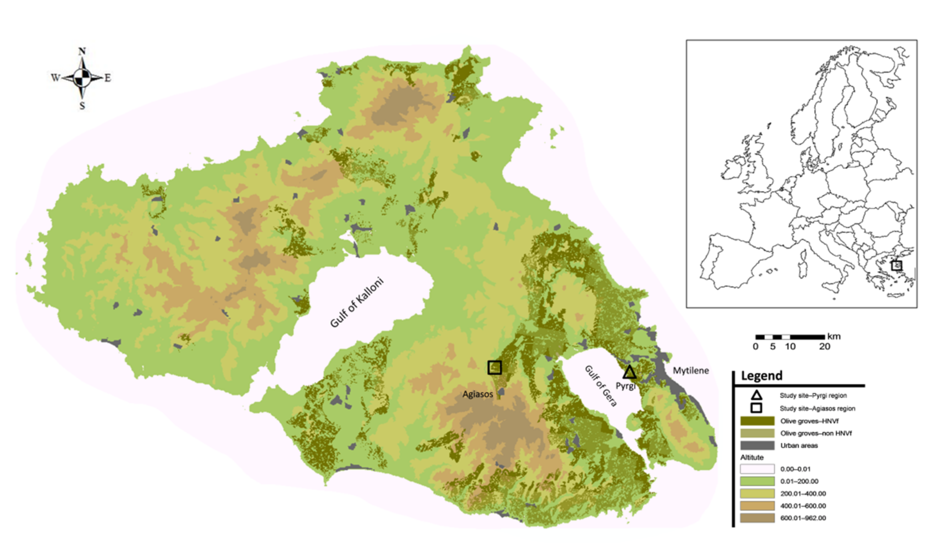
Our study represents the first attempt to monitor the pressures and the overall state of trees in traditional olive groves which are located on the island of Lesvos, within a part of the recognized European HNVf. For this, a crucial step was to separate the island’s extensive olive groves into traditional and nontraditional. However, their identification was challenging, as their exact boundaries were not mapped, and there was no accompanying information on the individual cultivation methods used at the grove level nor any information on criteria used to define each olive grove as a traditional one. Having determined the boundaries of the traditional olive groves, our analysis focused on areas with a clear long-term absence of cultivation practices so that we have the unequivocal image of the island’s traditionally grown olive tree state. After all, the agricultural landscape of the island of Lesvos has changed since the 1990s due to land abandonment [26] and, with it, cultivation practices have differentiated; nowadays, “cultivation” is often restricted to the mere harvest of olives. In some cases, pruning is also carried out, which abruptly modifies the vegetative–productive balance of the tree (pers. obs.). Therefore, an attempt was made to find traditional olive groves with clear features of cultivation practices of the past, obtaining a glimpse into the state of olive groves in the Mediterranean basin, as well as of Lesvos terraced groves, of previous decades [92]. These practices involved forming the trees’ shape to a great height and crown area, in order to overcome environmental stress and to produce larger biennial crops, by being able to accumulate water and nutrients in their large trunk and branches, and their extensive canopy and root system. Modern cultivation practices are substantially differentiated in terms of techniques (irrigation, fertilization, mechanical harvesting, pruning) [92] and shape of trees, aiming at low-growing irrigated trees, with a specific leaf area that produces a constant crop annually [30].

Having identified and located traditional olive groves, we introduced a comprehensive methodological framework for traditional olive grove productivity prediction, including both easily obtainable tree trait information, which can be recorded with simple tools even with the knowledge and experience of an average olive grower, and additional information obtained with more specialized, but noninvasive, tools and techniques. Contrary to intensive agricultural systems, assessing productivity in traditional olive groves is acceptable without continual monitoring of a large set of physiological and environmental variables because immediate interventions are not possible and, occasionally, even not desirable. It should be noted that traditional olive groves tend to be less easily accessible than more intensively grown olive groves, thus, minimizing the number of necessary field visits is important. We selected techniques that can be used to collect field data in one or a few sessions, at the correct time of year, to increase the applicability of our results by both growers and cooperatives as well as by land management and nature conservation authorities.

As the main concern of all those involved in olive growing is tree productivity, we placed particular emphasis on this parameter, bearing in mind that a typical olive tree in favorable environmental conditions and with the proper management practices (regular pruning, fertilization, soil management, pest and disease control) can be productively efficient for more than 100 years [93]. However, in traditional olive groves, in which the trees are much older, the absence of effective cultivation practices, in conjunction with biotic and abiotic pressures (e.g., phloem shoot-to-root flow depression due to wood decay), leads to inner crown leaf drop and retention of foliage on the outer part of the crown. Simultaneously, the inner branches start to be replaced by others on the outside and, thus, the available resources are invested in nonproductive structures [94,95], resulting in decreased productivity as trees trade reproductive for vegetative activity [30,95]. 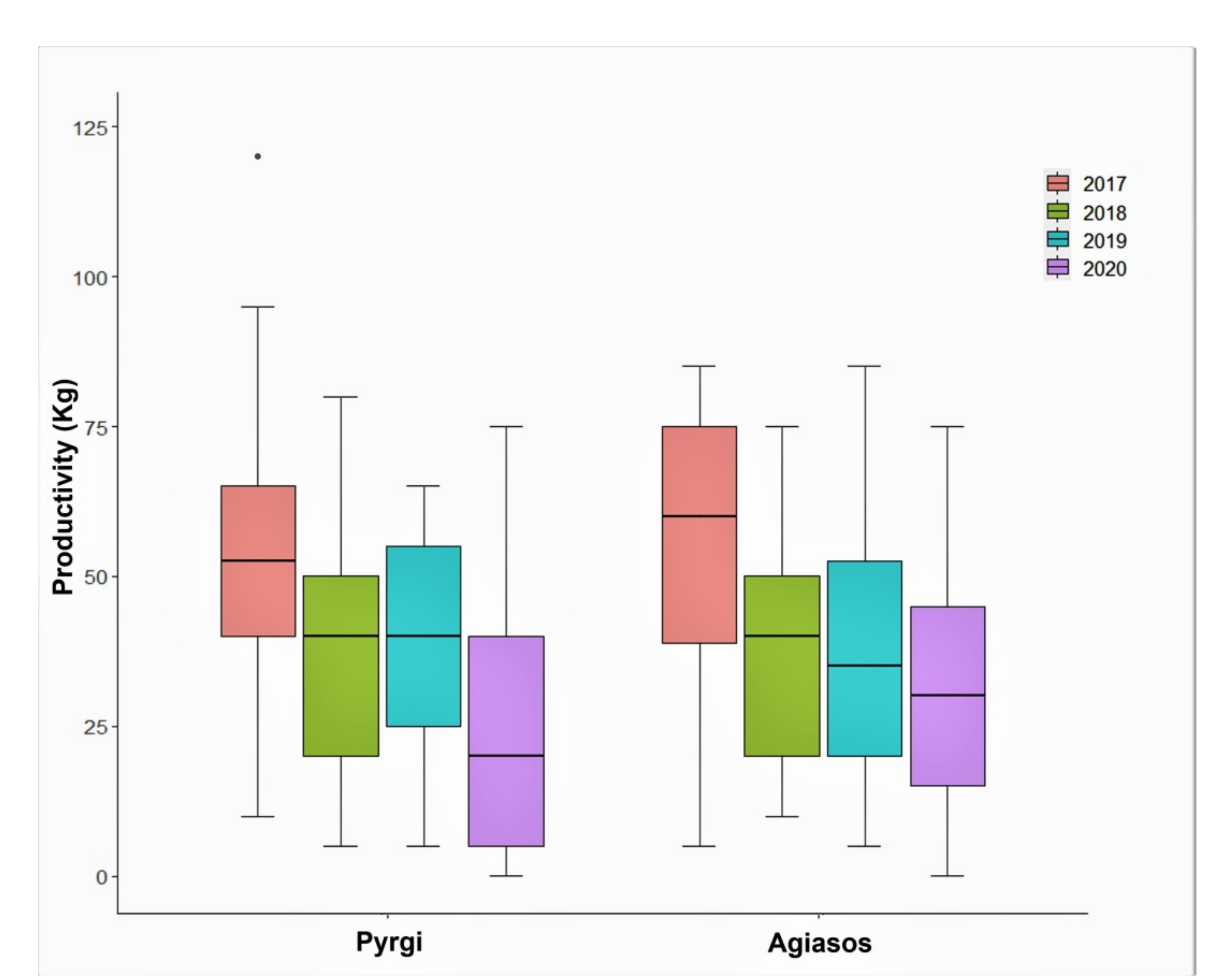Thus, in contrast with other studies [96,97], we took into account four consecutive years for estimating average annual productivity as well as the average renewal of productive shoots. Theoretically, we should be able to consider only two productivity years, due to biennial fruiting, but we noticed that, in our case, the alternate bearing was not very clear (Figure 4), so we chose to include all four years. Moreover, the activation of metabolic pathways related to the expression of alternate bearing is affected by a wide range of climatic events which influence the vegetative and reproductive development of olives [98], especially traditional ones, which we could not control.

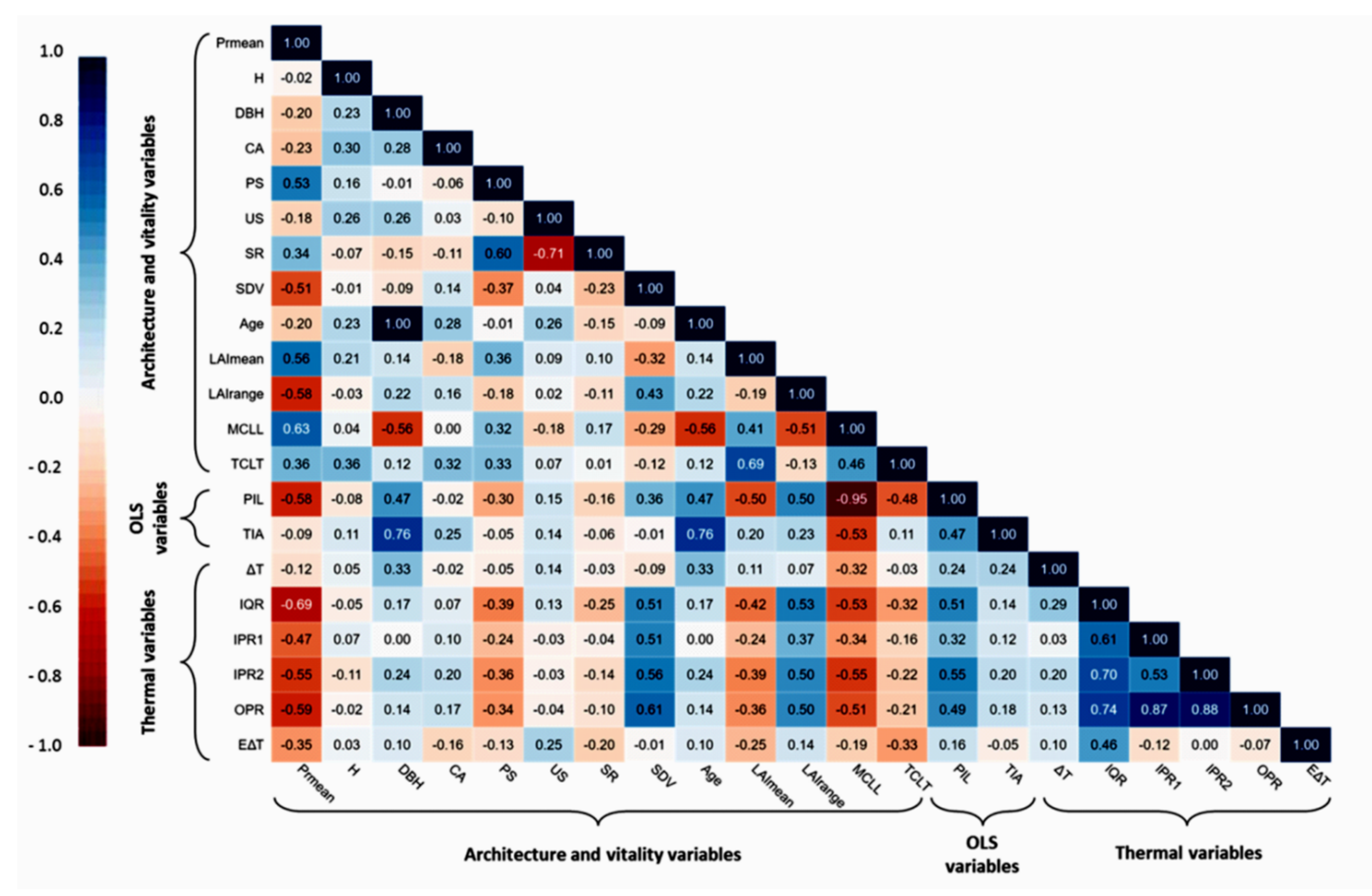
The investigation of the relationship between productivity and the architecture and vitality traits of the olive trees revealed significant evidence in linking these traits and with traditional olive grove functioning as a productive system. Of the twelve distinct traits that were either measured or calculated (e.g., MCL_L, TCL_T), five were found to be positively related (PS, SR, LAI_mean, MCL_L, TCL_T) and two negatively related (SDV, LAI_range) to productivity (Figure 5). Resistance mechanisms against biotic and abiotic stressors are reduced in aged olive trees [99], such as ours, and physiological adaptation mechanisms (e.g., high photosynthetic rate with low stomatal conductance) are affected by reduced vegetative activity [100,101]; these effects are compatible with the negative productivity relationships with OLS variables.

On the one hand, the highest positive correlations which were observed between productivity and MCL_L and LAI_mean confirmed the already established view that these traits are considered ideal biophysical indices for the description of these relationships [102]. Regarding MCL_L, it is well known that, despite being the essential driver of photosynthesis, and consequently olive productivity, it should be used in combination with LAI [103], which is an important criterion in evaluating olive trees’ state, as it shows the degree to which a tree can photosynthesize. In our case, the LAI_mean for the 80 olive trees was particularly low (2.11 ± 0.75), compared with the optimal value of 6 for achieving high olive yields [30]. Apart from this, we consider that the LAI values that we found are more representative of old, rather than young, olive groves, as similar studies for measuring LAI in an old olive grove in Italy found a value of 3.5 [104] and, in an intensive mature grove in Tunisia, a value of 2.8 [105].

On the other hand, the negative correlations between productivity and SDV and LAI_range, and both the relationship between them (r = 0.427; p < 0.0001) and their relationship with other significant traits (e.g., MCL_L, PIL), identify two very important parameters for estimating olive tree health. To the best of our knowledge, there is no other relevant study to use both of these traits as estimators of olive tree health. Nevertheless, we consider that it is of great importance, as LAI_range highlighted the deviation of olive trees from a healthy state, with extreme differences in LAI values taken into account, while SDV estimated the possible extent of the trees’ phloem shoot-to-root flow depression, by quantifying its structural abnormalities. In parallel, SDV is a crucial connecting link between olive tree vitality metrics and infrared thermography; it describes trunk growth patterns, which may exhibit cracks, wounds, detached bark, and cankers, and it shows a positive correlation with almost all the thermal statistical variables which describe the thermal profile of olive trees (Figure 5).

These relationships result from olive tree hydraulic physiology, as olive trees have developed different strategies to sustain a balance between water supply and water loss [106], by either adapting their leaf and root distribution [107] or by entire branch failure [108]. Regarding their trunks, the alteration of their hydraulic properties due to less plasticity leads to interrupting the water supply to all trunks’ neighboring segments [109]. 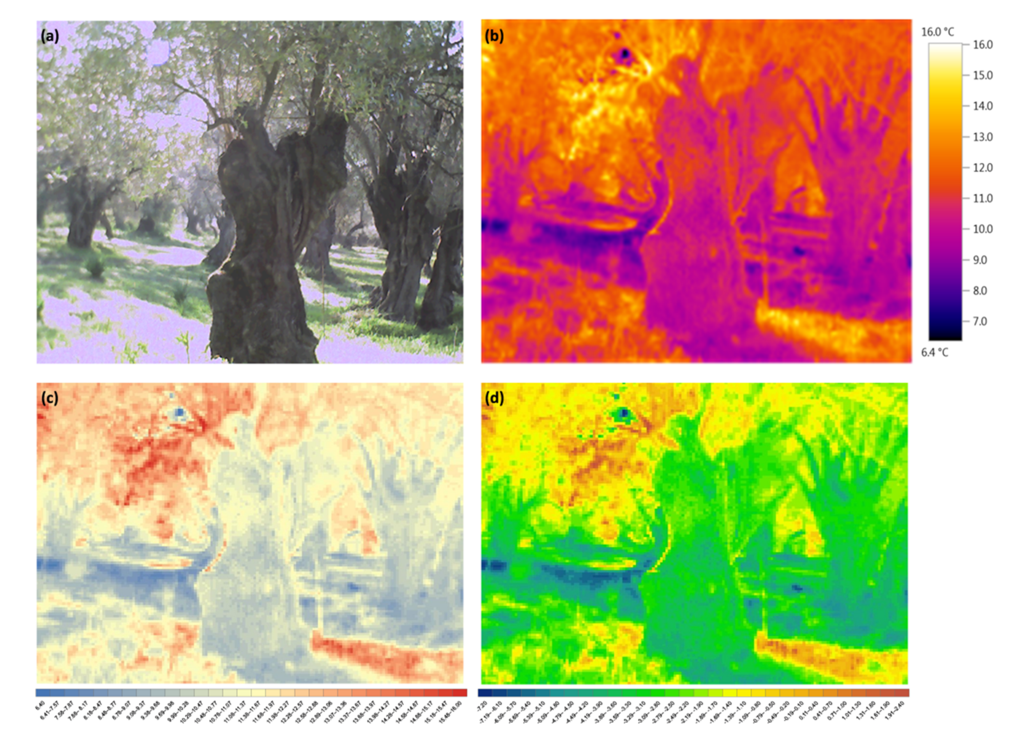Thus, possible hydraulic failure in conductive tissues, related to both water supply conditions and xylem anatomical characteristics [110], causes the surface temperature of the tree trunk to fluctuate [111] and reflects tree health. IRT can detect these fluctuations, indicating potential disturbances, when temperature distribution is uneven, or a healthy state when surface temperature is homogenous [56,112]. In our case, the exported thermal variables allowed the reliable detection of SDV, while their association with other significant phenotypic traits provided critical insights into the conservation state of traditional olive groves.

Given the prominence of traditional olive groves both on the island of Lesvos and in other parts of Greece [113], a detailed analysis regarding their productivity estimation based on both trees’ phenotypic traits and their thermal properties is required. However, for productivity assessment, it is important to take into account the possible susceptibility of traditionally grown olive trees to disease infestations. In this context, we have created a suite of important features, derived from the linear and the logistic models, which can satisfactorily explain traditional olive grove dynamics.

The high explanatory nature of the four linear models, using different predictor groups, showed that the four-year average productivity of the traditional olive trees can be explained to a very high degree. This high explanatory power, as indicated by the coefficient of determination values, especially in the “architecture and vitality traits” model (R² = 0.610) and in the “combination” model (R² = 0.702), showed that there are specific features of olive trees that can disclose the variation levels of their productivity (Table 2). We consider this to be extremely important if one considers that parameters that would potentially enhance our models, such as slope and aspect at individual tree level, slope and aspect of terraced sites, soil nutrient content, and trees’ competition levels, which were essential in other predictive models for olive tree productivity [97], were not taken into account. The separate examination of each harvest season, although with a lower explanatory power in three out of four years, followed a similar pattern: the “architecture and vitality traits” and the “combination” models showed an explanatory power ranging from 41.5% to 60.2% (Table A2, Table A3, Table A4 and Table A5).

It is noteworthy that, even though the model based on thermal variables showed moderate interpretive power in estimating of Pr_mean (R² = 0.463) (Table 2), lower still for individual years (24.5–35.4%) (Table A2, Table A3, Table A4 and Table A5), infrared thermography appears to be a valuable method for obtaining precise data for productivity estimation. Among the extracted thermal variables, only IQR had an important contribution to Pr_mean in the “thermal” model, while in the “combination” model, IQR showed the third-largest unique contribution (5.4%) out of the six predictive factors. Additionally, the negative coefficient of IQR demonstrates an inverse relationship of IQR with productivity, supporting the view that a uniform tree trunk surface temperature distribution is associated with a healthy tree state and higher productivity.

The dependence of productivity from OLS severity metrics indicated a moderate to low inverse effect (R² = 0.368; Table 2), which strengthens the argument, also reported by MacDonald et al. [114], that this fungal disease is probably responsible for the reported low productivity of the infected olive trees. Indeed, by repeating the multiple linear regression with the poor condition group of trees (G3), the explanatory power of the model rises to 46.5% (F (2, 19) = 18.41, p < 0.001, R² = 0.465), having TIA as the only statistically significant explanatory variable in the final model. Following the same procedure for the G1 and G2 groups did not yield any significant results. The age of the G3 olive trees (300.60 ± 84.62 years) also played an important role; controlling for the effect of age, the correlation of Pr_mean with PIL had a negative nonsignificant coefficient (r = −0.44; p = 0.053) and a positive nonsignificant coefficient with TIA (r = 0.26; p = 0.254).

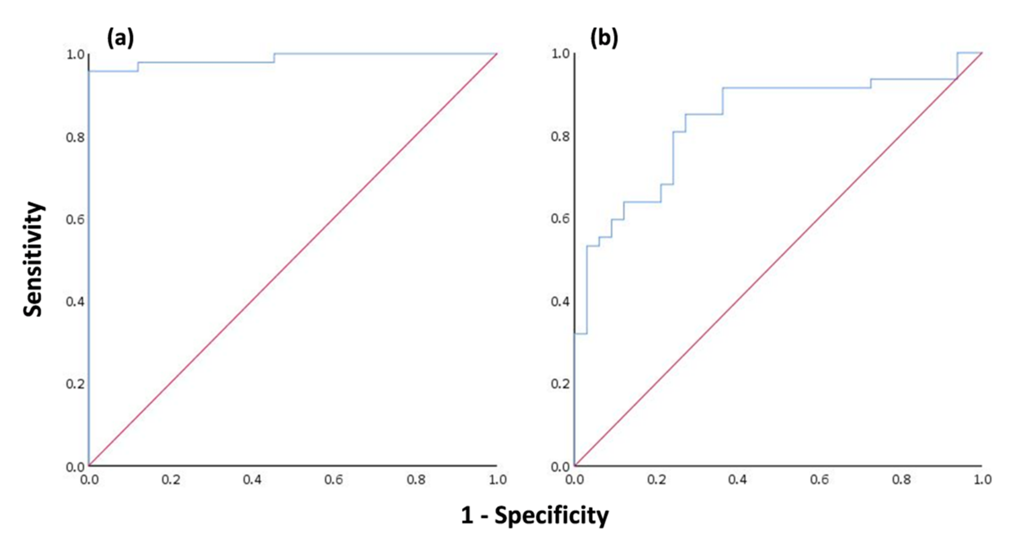
Assessing the olive tree infection by OLS indicated that 58.75% of the studied trees were infected. The presence of fungal pathogens is difficult to control as their populations show spatiotemporal and genetic variability, depending, to a large extent, on humidity and ambient temperature, while climate change increases the risk of infection in trees [115]. The logistic regression models had a high discriminatory performance and were quite informative regarding the predictors of both architecture and vitality traits and thermal variables groups, indicating that the probability of OLS infection could be predicted accurately by MCL_L and IQR. On the extremely high predicted classification accuracy of MCL_L (95.7%), trees with no symptoms presented a mean MCL_L of 0.98 ± 0.03 g/m², while those classified as infected had a much lower value of MCL_L (0.73 ± 0.14 g/m²). This differentiation occurs as the infected leaves undertake a gradual deterioration of their cytoplasmic contents, resulting in the degradation of chloroplasts and the progressive disappearance of chlorophyll [116]. From the standpoint of assessing OLS presence using thermal variables, it is understood that both the classification accuracy (80%) and the degree of explanatory power of the model (39%) are not ideal to suggest the use of IRT for detecting infection in olive trees. However, we must keep in mind that the examined thermal variables (IQR) (a) had a substantial difference between infected (0.85 ± 0.38) and noninfected trees (0.55 ± 0.13), and (b) were calculated from infrared images of the tree trunk and not from the leaves, which is the main organ that this disease affects. In addition, IRT has been proved to be a valuable method for identifying biotic stresses by analyzing temperature alterations in plant leaves [44].

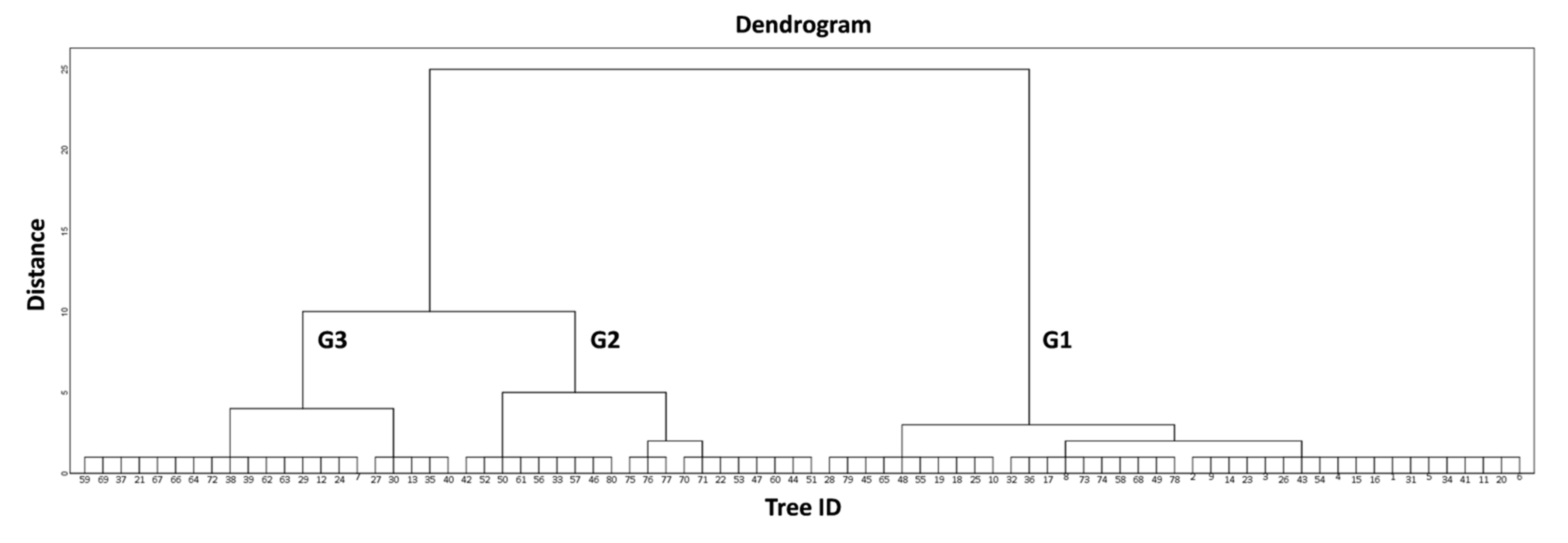
The classification of the 80 trees in three classes (G1, G2, G3) enabled tree health state categorization at a population level, as the group G1 includes olive trees that are in a good condition, G2 includes trees in an intermediate state, and group G3 contains trees which are in poor condition. Moreover, specific traits of the olive trees’ groups can be adequately described, to some extent, by the extracted thermal variables, as shown by the initial examination of the relationships between them (Figure 5). In particular, it is noted that G1 and G3 display the lowest and highest values in all thermal variables, respectively, while G2 lies somewhere in between, except for ΔT (Table 4).

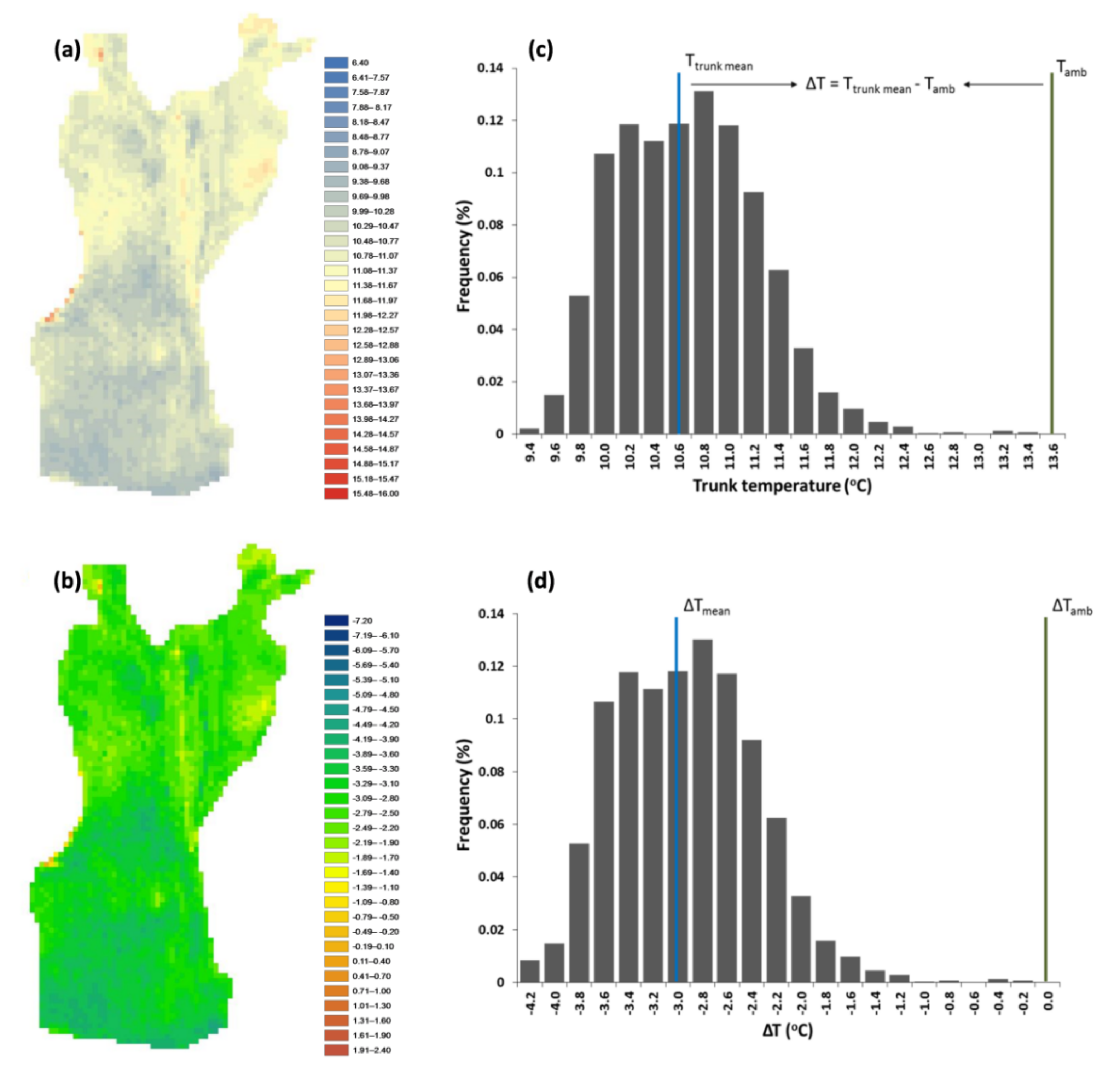
The high ΔT value of the G3 trees indicated their low temperature distance from T_amb; this means that the tree trunk has a faster response to ambient temperature indicative of hollows within the trunk where the air enters and heats the trunk surface faster. Paradoxically, regarding a particularly important thermal variable describing the actual extent of defect patches (ΕΔΤ), we did not find any statistically significant differences between the examined groups (F (2, 77) = 2.97, p = 0.057); this suggests that the area of any abnormalities is not as important, at least for traditional olive groves, as their intensity, described by the IQR for the whole tree and by the OPR for individual elements of the trunk. Hence, the three classes that describe the health state of olive trees (good, intermediate, poor) correspond to specific value ranges of these thermal variables. Poor condition corresponds to the highest values of the extracted thermal variables, while good condition corresponds to the lowest values.

Thus, combining the results of productivity assessment, infected trees’ identification, and hierarchical classification, we can conclude that mainly IQR and secondarily OPR can be considered as indicators of olive trees’ health state. The low value of these indices confirms the homogeneous temperature distribution on the tree trunk, as originally described by Catena and Catena [56], and identifies high values of vitality traits simultaneously with the absence of the OLS disease. Therefore, these indices are appropriate for measuring the thermal profile of each olive tree and for assessing its health state.

In conclusion, our results provide evidence for a combinatory methodological framework for traditional olive grove productivity prediction, taking into account typical phenotypic, spectral, and thermal tree traits. We further demonstrate that it is possible to detect the incidence of OLS in traditional olive groves and to classify olive trees into different health state categories using the same variables. Although infrared images did not provide the best prediction of tree productivity, nor the optimal classification for OLS incidence, nonetheless, they could give satisfactory information for a rapid first assessment of the health and productivity of a traditional olive grove noninvasively. Combined with long-established methods and tools of assessing health and productivity, such as LAI and chlorophyll concentration, they can further improve the predictive power to a very high level. Overall, this study establishes a foundation for the design and application of appropriate management measures of traditional olive groves using a relatively simple and time-saving, but sufficiently accurate, methodology.

References

1. Altieri, M.A. Linking Ecologists and Traditional Farmers in the Search for Sustainable Agriculture. Front. Ecol. Environ. 2004, 2, 35. [Google Scholar] [CrossRef]
2. Jarvis, D.; Brown, A.H.D.; Cuong, P.H.; Collado-Panduro, L. A global perspective of the richness and evenness. Proc. Natl. Acad. Sci. USA 2008, 105, 5326–5331. [Google Scholar] [CrossRef] [Green Version]
3. Achtak, H.; Ater, M.; Oukabli, A.; Santoni, S.; Kjellberg, F.; Khadari, B. Traditional agroecosystems as conservatories and incubators of cultivated plant varietal diversity: The case of fig (Ficus carica L.) in Morocco. BMC Plant Biol. 2010, 10, 28. [Google Scholar] [CrossRef] [Green Version]
4. Fischer, J.; Hartel, T.; Kuemmerle, T. Conservation policy in traditional farming landscapes. Conserv. Lett. 2012, 5, 167–175. [Google Scholar] [CrossRef] [Green Version]
5. Beaufoy, G.; Jones, G. HNV Farming in England and Wales–Findings from Three Local Projects; EFNCP: Portree, UK, 2012; ISBN 9781902855011. [Google Scholar]
6. Plieninger, T.; Bieling, C. Resilience-Based Perspectives to Guiding High-Nature-Value Farmland through Socioeconomic Change. Ecol. Soc. 2013, 18, 4. [Google Scholar] [CrossRef] [Green Version]
7. Lomba, A.; Guerra, C.; Alonso, J.; Honrado, J.P.; Jongman, R.; McCracken, D. Mapping and monitoring High Nature Value farmlands: Challenges in European landscapes. J. Environ. Manag. 2014, 143, 140–150. [Google Scholar] [CrossRef] [PubMed]
8. Loumou, A.; Giourga, C. Olive groves: The life and identity of the Mediterranean. Agric. Hum. Values 2003, 20, 87–95. [Google Scholar] [CrossRef]
9. Solomou, A.; Sfougaris, A. Comparing conventional and organic olive groves in central Greece: Plant and bird diversity and abundance. Renew. Agric. Food Syst. 2011, 26, 297–316. [Google Scholar] [CrossRef]
10. Price, M. High Nature Value Farming in Europe: 35 European Countries—Experiences and Perspectives. Mt. Res. Dev. 2013, 33, 480. [Google Scholar] [CrossRef]
11. Pointereau, P.; Paracchini, M.L.; Terres, J.-M.; Jiguet, F.; Bas, Y.; Biala, K. Identification of High Nature Value Farmland in France through Statistical Information and Farm Practice Surveys; Report EUR 22786 EN; Publications Office of the EU: Luxembourg, 2007; ISBN 9789279064753. [Google Scholar]
12. Poláková, J.; Tucker, G.; Hart, K.; Dwyer, J.; Rayment, M. Addressing Biodiversity and Habitat Preservation through Measures Applied under the Common Agricultural Policy; Report Prepared for DG Agriculture and Rural Development, Contract No. 30-CE-0388497/00-44; Institute for European Environmental Policy: London, UK, 2011. [Google Scholar]
13. Keenleyside, C.; Beaufoy, G.; Tucker, G.; Jones, G. High Nature Value Farming Throughout EU-27 and Its Financial Support under the CAP. 2014; Report Prepared for DG Environment, Contract No ENV B.1/ETU//0035; Institute for European Environmental Policy: London, UK, 2014. [Google Scholar]
14. Duarte, F.; Jones, N.; Fleskens, L. Traditional olive orchards on sloping land: Sustainability or abandonment? J. Environ. Manag. 2008, 89, 86–98. [Google Scholar] [CrossRef]
15. Henle, K.; Alard, D.; Clitherow, J.; Cobb, P.; Firbank, L.; Kull, T.; McCracken, D.; Moritz, R.F.A.; Niemelä, J.; Rebane, M.; et al. Identifying and managing the conflicts between agriculture and biodiversity conservation in Europe—A review. Agric. Ecosyst. Environ. 2008, 124, 60–71. [Google Scholar] [CrossRef]
16. De Graaff, J.; Duarte, F.; Fleskens, L.; de Figueiredo, T. The future of olive groves on sloping land and ex-ante assessment of cross compliance for erosion control. Land Use Policy 2010, 27, 33–41. [Google Scholar] [CrossRef]
17. De Graaff, J.; Kessler, A.; Duarte, F. Financial consequences of cross-compliance and flat-rate-per-ha subsidies: The case of olive farmers on sloping land. Land Use Policy 2011, 28, 388–394. [Google Scholar] [CrossRef]
18. Lefebvre, M.; Espinosa, M.; Gomez-y-Paloma, S. The Influence of the Common Agricultural Policy on Agricultural Landscapes; Publications Office of the European Union: Luxembourg, 2012. [Google Scholar] [CrossRef]
19. Brandolini, P. The Outstanding Terraced Landscape of the Terre Coastal Slopes (Eastern Liguria); Soldati, M.M.M., Ed.; Springer: Cham, Switzerland, 2017; ISBN 9783319261928. [Google Scholar]
20. Modica, G.; Praticò, S.; Di Fazio, S. Abandonment of traditional terraced landscape: A change detection approach (a case study in Costa Viola, Calabria, Italy). Land Degrad. Dev. 2017, 28, 2608–2622. [Google Scholar] [CrossRef]
21. Brunori, E.; Salvati, L.; Antogiovanni, A.; Biasi, R. Worrying about “vertical landscapes”: Terraced olive groves and ecosystem services in marginal land in central Italy. Sustainability 2018, 10, 1164. [Google Scholar] [CrossRef] [Green Version]
22. Benton, T.G.; Vickery, J.A.; Wilson, J.D. Farmland biodiversity: Is habitat heterogeneity the key? Trends Ecol. Evol. 2003, 18, 182–188. [Google Scholar] [CrossRef]
23. Hole, D.G.; Perkins, A.J.; Wilson, J.D.; Alexander, I.H.; Grice, P.V.; Evans, A.D. Does organic farming benefit biodiversity? Biol. Conserv. 2005, 122, 113–130. [Google Scholar] [CrossRef]
24. Fleskens, L. Conservation Scenarios for Olive Farming on Sloping Land in the Mediterranean. Ph.D. Thesis, Wageningen University, Wageningen, The Netherlands, 2007. [Google Scholar]
25. Caraveli, H. A comparative analysis on intensification and extensification in mediterranean agriculture: Dilemmas for LFAs policy. J. Rural Stud. 2000, 16, 231–242. [Google Scholar] [CrossRef]
26. Kizos, T.; Dalaka, A.; Petanidou, T. Farmers’ attitudes and landscape change: Evidence from the abandonment of terraced cultivations on Lesvos, Greece. Agric. Human Values 2010, 27, 199–212. [Google Scholar] [CrossRef]
27. Dunjó, G.; Pardini, G.; Gispert, M. Land use change effects on abandoned terraced soils in a Mediterranean catchment, NE Spain. Catena 2003, 52, 23–37. [Google Scholar] [CrossRef]
28. Salvati, L.; Ferrara, C. The local-scale impact of soil salinization on the socioeconomic context: An exploratory analysis in Italy. Catena 2015, 127, 312–322. [Google Scholar] [CrossRef]
29. Stanchi, S.; Freppaz, M.; Agnelli, A.; Reinsch, T.; Zanini, E. Properties, best management practices and conservation of terraced soils in Southern Europe (from Mediterranean areas to the Alps): A review. Quat. Int. 2012, 265, 90–100. [Google Scholar] [CrossRef] [Green Version]
30. International Olive Council. Production Techniques in Olive Growing; IOC: Madrid, Spain, 2007; ISBN 9788493166366. [Google Scholar]
31. Tartaglini, N.; Calabrese, G.J.; Servadei, L. Ancient olive orchards as high nature value farmland; A shared vision at euro-mediterranean level. In A Multi-Scale and Multi-Level Approach for Conservation of Ancient Olive Orchards in the Euro-Mediterranean Region; La Posta, A., Lacirignola, C., Mimiola, G., Eds.; CIHEAM Mediterranean Agronomic Institute: Bari, Italy, 2012; pp. 27–39. [Google Scholar]
32. Beaufoy, G. Olives Ecosystems and Biodiversity—Considerations for Action in the EU; IOC: Madrid, Spain, 2009; p. 26. [Google Scholar]
33. Zhang, J. Multi-source remote sensing data fusion: Status and trends. Int. J. Image Data Fusion 2010, 1, 5–24. [Google Scholar] [CrossRef] [Green Version]
34. Hansen, M.C.; Stehman, S.V.; Potapov, P.V.; Loveland, T.R.; Townshend, J.R.G.; DeFries, R.S.; Pittman, K.W.; Arunarwati, B.; Stolle, F.; Steininger, M.K.; et al. Humid tropical forest clearing from 2000 to 2005 quantified by using multitemporal and multiresolution remotely sensed data. Proc. Natl. Acad. Sci. USA 2008, 105, 9439–9444. [Google Scholar] [CrossRef] [PubMed] [Green Version]
35. Eva, H.; Carboni, S.; Achard, F.; Stach, N.; Durieux, L.; Faure, J.F.; Mollicone, D. Monitoring forest areas from continental to territorial levels using a sample of medium spatial resolution satellite imagery. ISPRS J. Photogramm. Remote Sens. 2010, 65, 191–197. [Google Scholar] [CrossRef]
36. Huang, Y.; Ren, Z.; Li, D.; Liu, X. Phenotypic techniques and applications in fruit trees: A review. Plant Methods 2020, 16, 1–22. [Google Scholar] [CrossRef]
37. Di Nisio, A.; Adamo, F.; Acciani, G.; Attivissimo, F. Fast detection of olive trees affected by xylella fastidiosa from uavs using multispectral imaging. Sensors 2020, 20, 4915. [Google Scholar] [CrossRef]
38. Castrignanò, A.; Belmonte, A.; Antelmi, I.; Quarto, R.; Quarto, F.; Shaddad, S.; Sion, V.; Muolo, M.R.; Ranieri, N.A.; Gadaleta, G.; et al. Semi-automatic method for early detection of xylella fastidiosa in olive trees using uav multispectral imagery and geostatistical-discriminant analysis. Remote Sens. 2021, 13, 14. [Google Scholar] [CrossRef]
39. Blekos, K.; Tsakas, A.; Xouris, C.; Evdokidis, I.; Alexandropoulos, D.; Alexakos, C.; Katakis, S.; Makedonas, A.; Theoharatos, C.; Lalos, A. Analysis, modeling and multi-spectral sensing for the predictive management of verticillium wilt in olive groves. J. Sens. Actuator Netw. 2021, 10, 15. [Google Scholar] [CrossRef]
40. Berry, J.K.; Delgado, J.A.; Khosla, R.; Pierce, F. Precision Conservation for Environmental Sustainability. J. Soil Water Conserv. 2003, 10, 1–26. [Google Scholar]
41. Berry, J.K.; Delgado, J.A.; Pierce, F.J.; Khosla, R. Applying spatial analysis for precision. J. Soil Water Conserv. 2005, 60, 363–370. [Google Scholar]
42. Delgado, J.A.; Berry, J.K. Advances in Precision Conservation. Adv. Agron. 2008, 98, 1–44. [Google Scholar] [CrossRef]
43. Ouis, D. Non Destructive Techniques for Detecting Decay in Standing Trees. Arboric. J. 2003, 27, 159–177. [Google Scholar] [CrossRef]
44. Ishimwe, R.; Abutaleb, K.; Ahmed, F. Applications of Thermal Imaging in Agriculture—A Review. Adv. Remote Sens. 2014, 3, 128–140. [Google Scholar] [CrossRef] [Green Version]
45. Dragavtsev, V.; Nartov, V.P. Application of Thermal Imaging in Agriculture and Forestry. Eur. Agrophys. J. 2015, 2, 15. [Google Scholar] [CrossRef] [Green Version]
46. Still, C.; Powell, R.; Aubrecht, D.; Kim, Y.; Helliker, B.; Roberts, D.; Richardson, A.D.; Goulden, M. Thermal imaging in plant and ecosystem ecology: Applications and challenges. Ecosphere 2019, 10, 6. [Google Scholar] [CrossRef] [Green Version]
47. Vadivambal, R.; Jayas, D.S. Applications of Thermal Imaging in Agriculture and Food Industry-A Review. Food Bioprocess Technol. 2011, 4, 186–199. [Google Scholar] [CrossRef]
48. Chaerle, L.; Van Caeneghem, W.; Messens, E.; Lambers, H.; Van Montagu, M.; Van Der Straeten, D. Presymptomatic visualization of plant-virus interactions by thermography. Nat. Biotechnol. 1999, 17, 813–816. [Google Scholar] [CrossRef] [PubMed]
49. Chaerle, L.; De Boever, F.; Van Montagu, M.; Van der Straeten, D. Thermographic visualization of cell death in tobacco and Arabidopsis. Plant Cell Environ. 2001, 24, 15–25. [Google Scholar] [CrossRef]
50. Lenthe, J.H.; Oerke, E.C.; Dehne, H.W. Digital infrared thermography for monitoring canopy health of wheat. Precis. Agric. 2007, 8, 15–26. [Google Scholar] [CrossRef]
51. Agam, N.; Cohen, Y.; Berni, J.A.J.; Alchanatis, V.; Kool, D.; Dag, A.; Yermiyahu, U.; Ben-Gal, A. An insight to the performance of crop water stress index for olive trees. Agric. Water Manag. 2013, 118, 79–86. [Google Scholar] [CrossRef]
52. Struthers, R.; Ivanova, A.; Tits, L.; Swennen, R.; Coppin, P. Thermal infrared imaging of the temporal variability in stomatal conductance for fruit trees. Int. J. Appl. Earth Obs. Geoinf. 2015, 39, 9–17. [Google Scholar] [CrossRef]
53. Egea, G.; Padilla-Díaz, C.M.; Martinez-Guanter, J.; Fernández, J.E.; Pérez-Ruiz, M. Assessing a crop water stress index derived from aerial thermal imaging and infrared thermometry in super-high density olive orchards. Agric. Water Manag. 2017, 187, 210–221. [Google Scholar] [CrossRef] [Green Version]
54. Oerke, E.C.; Fröhling, P.; Steiner, U. Thermographic assessment of scab disease on apple leaves. Precis. Agric. 2011, 12, 699–715. [Google Scholar] [CrossRef]
55. Ouledali, S.; Ennajeh, M.; Zrig, A.; Gianinazzi, S.; Khemira, H. Estimating the contribution of arbuscular mycorrhizal fungi to drought tolerance of potted olive trees (Olea europaea). Acta Physiol. Plant. 2018, 40, 1–13. [Google Scholar] [CrossRef]
56. Catena, A.; Catena, G. Overview of thermal imaging for tree assessment. Arboric. J. 2008, 30, 259–270. [Google Scholar] [CrossRef]
57. Guo, Y.Y.; Yu, H.Y.; Kong, D.S.; Yan, F.; Zhang, Y.J. Effects of drought stress on growth and chlorophyll fluorescence of Lycium ruthenicum Murr. seedlings. Photosynthetica 2016, 54, 524–531. [Google Scholar] [CrossRef]
58. Wang, J.; Wang, T.; Shi, T.; Wu, G.; Skidmore, A.K. A wavelet-based area parameter for indirectly estimating copper concentration in Carex leaves from canopy reflectance. Remote Sens. 2015, 7, 15340–15360. [Google Scholar] [CrossRef] [Green Version]
59. Obeidat, W.; Avila, L.; Earl, H.; Lukens, L. Leaf spectral reflectance of maize seedlings and its relationship to cold tolerance. Crop Sci. 2018, 58, 2569–2580. [Google Scholar] [CrossRef]
60. Li, W.; Sun, Z.; Lu, S.; Omasa, K. Estimation of the leaf chlorophyll content using multiangular spectral reflectance factor. Plant. Cell Environ. 2019, 42, 3152–3165. [Google Scholar] [CrossRef]
61. Ali, M.M.; Al-Ani, A.; Eamus, D.; Tan, D.K.Y. Leaf nitrogen determination using non-destructive techniques—A review. J. Plant Nutr. 2017, 40, 928–953. [Google Scholar] [CrossRef]
62. Steele, M.; Gitelson, A.A.; Rundquist, D. Nondestructive estimation of leaf chlorophyll content in grapes. Am. J. Enol. Vitic. 2008, 59, 299–305. [Google Scholar]
63. Pavlovic, D.; Nikolic, B.; Djurovic, S.; Waisi, H.; Andjelkovic, A.; Marisavljevic, D. Chlorophyll as a measure of plant health: Agroecological aspects. Pestic. Fitomed. 2014, 29, 21–34. [Google Scholar] [CrossRef]
64. Almansoori, T.; Salman, M.; Aljazeri, M. Rapid and nondestructive estimations of chlorophyll concentration in date palm (Phoenix dactylifera L.) leaflets using SPAD-502+ and CCM-200 portable chlorophyll meters. Emir. J. Food Agric. 2021, 33, 532–543. [Google Scholar] [CrossRef]
65. Richardson, A.D.; Duigan, S.P.; Berlyn, G.P. An evaluation of noninvasive methods to estimate foliar chlorophyll content. New Phytol. 2002, 153, 185–194. [Google Scholar] [CrossRef] [Green Version]
66. Mishra, K.B.; Mishra, A.; Klem, K. Govindjee Plant phenotyping: A perspective. Indian J. Plant Physiol. 2016, 21, 514–527. [Google Scholar] [CrossRef]
67. Sánchez-Reinoso, A.D.; Ligarreto-Moreno, G.A.; Restrepo-Díaz, H. Drought-tolerant common bush bean physiological parameters as indicators to identify susceptibility. HortScience 2019, 54, 2091–2098. [Google Scholar] [CrossRef] [Green Version]
68. Villalobos, F.J.; Testi, L.; Hidalgo, J.; Pastor, M.; Orgaz, F. Modelling potential growth and yield of olive (Olea europaea L.) canopies. Eur. J. Agron. 2006, 24, 296–303. [Google Scholar] [CrossRef]
69. Pelil, P.; Biradar, P.; Bhagawathi, A.U.; Hejjigar, I.S. Area Index of horticulture crops and its importance. Int. J. Curr. Microbiol. Appl. Sci. 2018, 7, 505–513. [Google Scholar]
70. Kosmas, C.; Danalatos, N.G.; Poesen, J.; Van Wesemael, B. The effect of water vapour adsorption on soil moisture content under Mediterranean climatic conditions. Agric. Water Manag. 1998, 36, 157–168. [Google Scholar] [CrossRef]
71. Marathianou, M.; Kosmas, C.; Gerontidis, S.; Detsis, V. Land-use evolution and degradation in Lesvos (Greece): A historical approach. Land Degrad. Dev. 2000, 11, 63–73. [Google Scholar] [CrossRef]
72. Paracchini, M.L.; Petersen, J.-E.; Hoogeveen, Y.; Bamps, C.; Burfield, I.; Van Swaay, C. High Nature Value Farmland in Europe—An Estimate of the Distribution Patterns on the Basis of Land Cover and Biodiversity Data; European Comission: Luxembourg, 2008; ISBN 9789279095689. [Google Scholar]
73. European Environment Agency (EEA). Corine Land Cover. Available online: https://land.copernicus.eu/pan-european/corine-land-cover/clc-2012 (accessed on 10 September 2017).
74. European Environment Agency (EEA). Tree Cover Density. Available online: https://land.copernicus.eu/pan-european/high-resolution-layers/forests/tree-cover-density (accessed on 10 September 2017).
75. European Environment Agency (EEA). Dominant Leaf Type. Available online: https://land.copernicus.eu/pan-european/high-resolution-layers/forests/dominant-leaf-type (accessed on 10 September 2017).
76. Pretzsch, H.; Biber, P.; Uhl, E.; Dahlhausen, J.; Rötzer, T.; Caldentey, J.; Koike, T.; van Con, T.; Chavanne, A.; Seifert, T.; et al. Crown size and growing space requirement of common tree species in urban centres, parks, and forests. Urban For. Urban Green. 2015, 14, 466–479. [Google Scholar] [CrossRef] [Green Version]
77. Ryan, M.G.; Binkley, D.; Fownes, J.H. Age-related decline in forest productivity: Pattern and process. Adv. Ecol. Res. 1997, 27, 213–262. [Google Scholar]
78. Fabbri, A.; Bartolini, G.; Lambardi, M.; Kailis, S.G. Olive Propagation Manual; CSIRO Publishing: Collingwood, VA, Australia, 2004; ISBN 0-643-06676-4. [Google Scholar]
79. Cherubini, P.; Gartner, B.L.; Tognetti, R.; Bräker, O.U.; Schoch, W.; Innes, J.L. Identification, measurement and interpretation of tree rings in woody species from mediterranean climates. Biol. Rev. Camb. Philos. Soc. 2003, 78, 119–148. [Google Scholar] [CrossRef] [Green Version]
80. Arnan, X.; López, B.C.; Martínez-Vilalta, J.; Estorach, M.; Poyatos, R. The age of monumental olive trees (Olea europaea) in northeastern Spain. Dendrochronologia 2012, 30, 11–14. [Google Scholar] [CrossRef]
81. Parry, C.; Blonquist, J.M.; Bugbee, B. In situ measurement of leaf chlorophyll concentration: Analysis of the optical/absolute relationship. Plant Cell Environ. 2014, 37, 2508–2520. [Google Scholar] [CrossRef]
82. Nauš, J.; Prokopová, J.; Řebíček, J.; Špundová, M. SPAD chlorophyll meter reading can be pronouncedly affected by chloroplast movement. Photosynth. Res. 2010, 105, 265–271. [Google Scholar] [CrossRef] [PubMed]
83. Masmoudi-Charfi, C.; Ben Mechlia, N. Characterization of young olive trees growth during the first six years of cultivation. Adv. Hortic. Sci. 2007, 21, 116–124. [Google Scholar] [CrossRef]
84. Salman, M. Biological control of Spilocaea oleagina, the causal agent of olive leaf spot disease, using antagonistic bacteria. J. Plant Pathol. 2017, 99, 741–744. [Google Scholar] [CrossRef]
85. Obanor, F.O.; Jaspers, M.V.; Jones, E.E.; Walter, M. Greenhouse and field evaluation of fungicides for control of olive leaf spot in New Zealand. Crop Prot. 2008, 27, 1335–1342. [Google Scholar] [CrossRef]
86. Sanei, S.J.; Razavi, S.E. Survey of Spilocaea oleagina, causal agent of olive leaf spot, in North of Iran. J. Yeast Fungal Res. 2011, 2, 33–38. [Google Scholar] [CrossRef]
87. Minkina, W.; Dudzik, S. Infrared Thermography: Errors and Uncertainties; John Wiley & Sons, Ltd.: Chichester, UK, 2009; ISBN 9780470747186. [Google Scholar]
88. Briscoe, N.J.; Handasyde, K.A.; Griffiths, S.R.; Porter, W.P.; Krockenberger, A.; Kearney, M.R. Tree-hugging koalas demonstrate a novel thermoregulatory mechanism for arboreal mammals. Biol. Lett. 2014, 10, 20140235. [Google Scholar] [CrossRef] [Green Version]
89. Idso, S.B.; Reginato, R.J.; Jackson, R.D.; Pinter, P.J. Measuring yield-reducing plant water potential depressions in wheat by infrared thermometry. Irrig. Sci. 1981, 2, 205–212. [Google Scholar] [CrossRef]
90. Zuur, A.F.; Ieno, E.N.; Elphick, C.S. A protocol for data exploration to avoid common statistical problems. Methods Ecol. Evol. 2010, 1, 3–14. [Google Scholar] [CrossRef]
91. Youden, W.J. Index for rating diagnostic tests. Cancer 1950, 3, 32–35. [Google Scholar] [CrossRef]
92. Lo Bianco, R.; Proietti, P.; Regni, L.; Caruso, T. Planting systems for modern olive growing: Strengths and weaknesses. Agric. 2021, 11, 494. [Google Scholar] [CrossRef]
93. Ozturk, M.; Altay, V.; Gönenç, T.M.; Unal, B.T.; Efe, R.; Akçiçek, E.; Bukhari, A. An overview of olive cultivation in Turkey: Botanical features, eco-physiology and phytochemical aspects. Agronomy 2021, 11, 295. [Google Scholar] [CrossRef]
94. Fernandez Escobar, R.; de la Rosa, R.; Leon, L.; Gomez, J.A.; Testi, F.; Orgaz, M.; Gil-Ribes, J.A.; Quesada-Moraga, E.; Trapero, A. Evolution and sustainability of the olive production systems. In Present and Future of the Mediterranean Olive Sector; Arcas, N., Arroyo López, F.N., Caballero, J., D’Andria, R., Fernández, M., Fernandez, E.R., Garrido, A., López-Miranda, J., Msallem, M., Parras, M., et al., Eds.; CIHEAM/IOC: Zaragoza, Spain, 2013; pp. 11–42. [Google Scholar]
95. Paoletti, A.; Rosati, A.; Famiani, F. Effects of cultivar, fruit presence and tree age on whole-plant dry matter partitioning in young olive trees. Heliyon 2021, 7, e06949. [Google Scholar] [CrossRef] [PubMed]
96. Sola-Guirado, R.R.; Castillo-Ruiz, F.J.; Jiménez-Jiménez, F.; Blanco-Roldan, G.L.; Castro-Garcia, S.; Gil-Ribes, J.A. Olive actual “on year” yield forecast tool based on the tree canopy geometry using UAS imagery. Sensors 2017, 17, 1743. [Google Scholar] [CrossRef] [Green Version]
97. Stateras, D.; Kalivas, D. Assessment of olive tree canopy characteristics and yield forecast model using high resolution uav imagery. Agriculture 2020, 10, 385. [Google Scholar] [CrossRef]
98. Lavee, S. Biennial bearing in olive (Olea europaea). Annales 2007, 17, 102–112. [Google Scholar]
99. Sofo, A.; Manfreda, S.; Fiorentino, M.; Dichio, B.; Xiloyannis, C. The olive tree: A paradigm for drought tolerance in Mediterranean climates. Hydrol. Earth Syst. Sci. 2008, 12, 293–301. [Google Scholar] [CrossRef] [Green Version]
100. Chartzoulakis, K.; Patakas, A.; Bosabalidis, A.M. Changes in water relations, photosynthesis and leaf anatomy induced by intermittent drought in two olive cultivars. Environ. Exp. Bot. 1999, 42, 113–120. [Google Scholar] [CrossRef]
101. Gargouri, K.; Bentaher, H.; Rhouma, A. A novel method to assess drought stress of olive tree. Agron. Sustain. Dev. 2012, 32, 735–745. [Google Scholar] [CrossRef] [Green Version]
102. Liu, Y.; Gong, W.; Xing, Y.; Hu, X.; Gong, J. Estimation of the forest stand mean height and aboveground biomass in Northeast China using SAR Sentinel-1B, multispectral Sentinel-2A, and DEM imagery. ISPRS J. Photogramm. Remote Sens. 2019, 151, 277–289. [Google Scholar] [CrossRef]
103. Heege, H.J. (Ed.) Precision in Crop Farming; Springer: Dordrecht, The Netherlands, 2013; ISBN 978-94-007-6759-1. [Google Scholar]
104. Čermák, J.; Gašpárek, J.; De Lorenzi, F.; Jones, H.G. Stand biometry and leaf area distribution in an old olive grove at Andria, southern Italy. Ann. For. Sci. 2007, 64, 491–501. [Google Scholar] [CrossRef]
105. Mezghani, M.A.; Hassouna, G.; Ibtissem, L.; Labidi, F. Leaf area index and light distribution in olive tree canopies (Olea europaea L.). Int. J. Agron. Agric. Res. 2016, 8, 60–65. [Google Scholar] [CrossRef]
106. Johnson, D.M.; Wortemann, R.; McCulloh, K.A.; Jordan-Meille, L.; Ward, E.; Warren, J.M.; Palmroth, S.; Domec, J.C. A test of the hydraulic vulnerability segmentation hypothesis in angiosperm and conifer tree species. Tree Physiol. 2016, 36, 983–993. [Google Scholar] [CrossRef] [Green Version]
107. Van Hees, A.F.M. Growth and morphology of pedunculate oak (Quercus robur L) and beech (Fagus sylvatica L) seedlings in relation to shading and drought. Ann. Sci. For. 1997, 54, 9–18. [Google Scholar] [CrossRef]
108. Rood, S.B.; Patiño, S.; Coombs, K.; Tyree, M.T. Branch sacrifice: Cavitation-associated drought adaptation of riparian cottonwoods. Trees Struct. Funct. 2000, 14, 248–257. [Google Scholar] [CrossRef]
109. Domec, J.C.; Lachenbruch, B.; Pruyn, M.L.; Spicer, R. Effects of age-related increases in sapwood area, leaf area, and xylem conductivity on height-related hydraulic costs in two contrasting coniferous species. Ann. For. Sci. 2012, 69, 17–27. [Google Scholar] [CrossRef] [Green Version]
110. López-Bernal, Á.; Alcántara, E.; Testi, L.; Villalobos, F.J. Spatial sap flow and xylem anatomical characteristics in olive trees under different irrigation regimes. Tree Physiol. 2010, 30, 1536–1544. [Google Scholar] [CrossRef] [Green Version]
111. Burcham, D.C.; Leong, E.C.; Fong, Y.K.; Tan, P.Y. An evaluation of internal defects and their effect on trunk surface temperature in Casuarina equisetifolia L. (Casuarinaceae). Arboric. Urban For. 2012, 38, 277–286. [Google Scholar] [CrossRef]
112. Omran, E.S.E. Early sensing of peanut leaf spot using spectroscopy and thermal imaging. Arch. Agron. Soil Sci. 2017, 63, 883–896. [Google Scholar] [CrossRef]
113. Giourga, C.; Loumou, A.; Tsevreni, I.; Vergou, A. Assessing the sustainability factors of traditional olive groves on Lesvos Island, Greece (Sustainability and traditional cultivation). GeoJournal 2008, 73, 149–159. [Google Scholar] [CrossRef]
114. MacDonald, A.J.; Walter, M.; Trought, M.C.; Frampton, C.M.; Burnip, G. Survey of olive leaf spot in New Zealand. N. Z. Plant Prot. 2000, 53, 126–132. [Google Scholar] [CrossRef] [Green Version]
115. Garrett, K.A.; Nita, M.; Wolf, E.D.D.; Gomez, L.; Sparks, A.H. Plant Pathogens as Indicators of Climate Change, 1st ed.; Elsevier: Amsterdam, The Netherlands, 2016; ISBN 9780444533012. [Google Scholar]
116. Lanza, B.; Ragnelli, A.M.; Priore, M.; Aimola, P. Morphological and histochemical investigation of the response of Olea europaea leaves to fungal attack by Spilocaea oleagina. Plant Pathol. 2017, 66, 1239–1247. [Google Scholar] [CrossRef]
Figure 1. Map of the island of Lesvos showing the two study sites and the distribution of olive groves within and outside the island’s HNVf.
Sustainability 14 00391 g001
Figure 2. Main methodological procedure of an individual olive tree sample for extracting the trunk temperature data: upper left is the RGB (visible) image (a); upper right is the infrared image after calibration using the TESTO software (b); lower left is the calibrated image after imported in ArcGIS, as a raster layer (c); lower right is the final infrared image (d), as a raster layer, after converting each pixel to correspond to the temperature difference of the tree trunk from the environment (ΔΤpixel).
Sustainability 14 00391 g002
Figure 3. Trunk of an individual olive tree sample which was exported with the use of ArcGIS Analysis toolbox, as well as the histogram of its pixel values; (a,c) refers to the actual trunk temperature along with its histogram, while (b,d) refers to the trunk ΔT along with its histogram distribution. The blue line in the two histograms corresponds to the mean trunk (c) and ΔT (d) temperature values. The green line corresponds to Tamb in both histograms.
Sustainability 14 00391 g003
Figure 4. Box plot showing the mean annual productivity for the four harvest seasons. Horizontal lines: medians; boxes: interquartile ranges (25–75%); whiskers: data ranges.
Sustainability 14 00391 g004
Figure 5. Pearson’s r correlation matrix showing the relationships between olive tree architectural, vitality, OLS, and thermal variables. For clarity, CCI, which refers to leaves, is omitted. Red and blue colors indicate positive and negative correlations, respectively, while intensity of color indicates the strength of the relationship. All correlation coefficients above 0.3 or below −0.3 are statistically significant (p < 0.05).
Sustainability 14 00391 g005
Figure 6. Dendrogram of the 80 olive trees that illustrates the dissimilarity as evaluated between Pyrgi and Agiasos sites. Numbers along branches indicated different groups.
Sustainability 14 00391 g006