Article

Hybrid Bayesian Network Models to Investigate the Impact of Built Environment Experience before Adulthood on Students’ Tolerable Travel Time to Campus: Towards Sustainable Commute Behavior

1
School of Architecture, Hunan University, Changsha 410012, China
2
School of Architecture and Urban Planning, Hunan City University, Yiyang 413002, China
3
Centre for Sustainable Urban Planning and Real Estate (SUPRE), Department of Urban and Regional Planning, Faculty of Built Environment, University of Malaya, Kuala Lumpur 50603, Malaysia
4
Department of Civil and Environmental Engineering, Universiti Teknologi Petronas, Seri Iskandar 32610, Malaysia
5
Department of Mechanical Equipment, Belgorod State Technological University Named after V.G. Shukhov, 308012 Belgorod, Russia
6
Department of Structural and Design Engineering, Kazan Federal University, 420008 Kazan, Russia
7
Department of Energy Supply of Enterprises, Construction of Buildings and Structures, Kazan State Power Engineering University, 420066 Kazan, Russia
8
Moscow State University of Technologies and Management (FCU), 109004 Moscow, Russia
9
Far Eastern Federal University, 690922 Vladivostok, Russia
10
Peter the Great St. Petersburg Polytechnic University, 195251 St. Petersburg, Russia
*
Authors to whom correspondence should be addressed.
Sustainability 2022, 14(1), 325; https://doi.org/10.3390/su14010325
Submission received: 24 November 2021 / Revised: 18 December 2021 / Accepted: 23 December 2021 / Published: 29 December 2021
(This article belongs to the Collection Urban Street Networks and Sustainable Transportation)

Abstract

:
This present study developed two predictive and associative Bayesian network models to forecast the tolerable travel time of university students to campus. This study considered the built environment experiences of university students during their early life-course as the main predictors of this study. The Bayesian network models were hybridized with the Pearson chi-square test to select the most relevant variables to predict the tolerable travel time. Two predictive models were developed. The first model was applied only to the variables of the built environment, while the second model was applied to all variables that were identified using the Pearson chi-square tests. The results showed that most students were inclined to choose the tolerable travel time of 0–20 min. Among the built environment predictors, the availability of residential buildings in the neighborhood in the age periods of 14–18 was the most important. Taking all the variables into account, distance from students’ homes to campuses was the most important. The findings of this research imply that the built environment experiences of people during their early life-course may affect their future travel behaviors and tolerance. Besides, the outcome of this study can help planners create more sustainable commute behaviors among people in the future by building more compact and mixed-use neighborhoods.

1. Introduction

Travel time (TT) is viewed as a necessary university-related activity and functions as a link between home and university campus. For each student, travel to campus differs in distance and complexity. This complexity may be increased if certain activities which link the travel and family are incorporated (e.g., the school operated or residential location decisions when spouses in households pursue careers) according to Wheatley [1]. This travel time spent can be regarded as both “productive” and a “waste of time”.
Several studies identified the associations between duration of travel and individuals’ well-being, including stress, comfort and satisfaction, and health [2,3,4,5]. In addition, several studies assessed the relationship between the TT and all daily activities and work duration [6,7]. Many factors, including sociodemographic, household characteristics, and travel mode, may influence TT [8]. In addition, many academic studies analyzed the reciprocity between built environment (BE) attributes and the TT [9,10,11,12,13,14].
As regards to the university students, there are some studies which considered TT as a function of students’ commute mode choice [15,16,17,18,19]. However, no available study has ever assessed the influence of BE factors on the students’ TT, and also, no study has ever considered the tolerable travel time (TTT) of university students considering the effects of BE variables. While a sizeable number of literature considered the effects of BE attributes on TT of the general population, studies on university students that exhibited different travel behaviors from the general population are still lacking [20,21,22].
The concept of TTT was developed by Milakis et al. [23]. This concept was established based on various theories related to commuting time, which include satisfaction [24,25], consideration sets [26], the travel time budget [27,28], and ideal travel time [29]. Milakis, Cervero, Van Wee, and Maat [23] employed semi-structured interviews to explore the primary characteristics of acceptable travel time (ATT). The study supported the validity of the concept of ATT through their findings and showed that the ATT may be varied for people with different sociodemographic attributes and travel modes. According to this concept, people presumably consider an ATT in their trips and decision-making processes regarding destinations. This concept views ATT as a behavioral threshold that is defined by the process of utilitarianism (i.e., intrinsic and derived utility). Intrinsic utility refers to the travel-related advantages (or disadvantages), while the advantages concerning activity at a journey destination are referred to as the derived utility. The concept splits the timeline of a one-way trip into three main periods in terms of total utility changes: (1) growth, (2) tolerance, and (3) decay. In the growth phase, both intrinsic and derived utility witnessed total utility increase. In the tolerance phase, the total utility yet increases, but slower than before until it touches the ATT (maximum level). Compared to the growth period, intrinsic utility is reduced and derived utility rises, but at a slower rate. Eventually, in the decay period, the total utility decreases because of the rapid decrease in intrinsic utility coupled with slow growth in derived utility.
The TTT, in fact, is the duration between the ideal travel time and ATT. In simple terms, TTT refers to the maximum amount of one-way TT that an individual tolerates [30]. If the actual TTs of a commuter reach or exceed the tolerance thresholds, the commuter is keen to decrease his/her travel time by making some changes, including, but not limited to, residential, job locations, or travel modes. The literature acknowledged the negative effects of exceeding the TTT thresholds. These impacts may be increasing stress levels, demanding excessive energy, and consuming time which may limit the time available for other daily activities [31,32,33,34,35,36,37].
There has been growing acknowledgement that travel behaviors are habitual [38,39,40] and these behaviors may become debilitated when disturbed by a contextual adjustment [39]. These contexts may comprise the environment where behavior occurs, such as social, physical, spatial, and time cues. Moreover, major life events (e.g., change in employment) may change the travel behaviors of individuals over time [41]. To date, several studies have examined the impacts of changes in life events and residential locations on the travel behavior of individuals [42,43,44,45,46,47]. However, many of these studies focused on predicting the travel mode choice, and many other aspects of travel outcomes, such as TTT, were overlooked. Furthermore, other phenomena that occurred to individuals in the past have received less attention. For example, no study has considered the associations between adults’ travel behavior outcomes and their living environments and BE experiences during childhood and adolescence. Several studies pointed out that previous living environments of people may influence their future behaviors that are related to commuting, such as their adaption and tolerance of crowding or their concern over the environment [48,49,50]. More importantly, lifetime habits, such as physically active lifestyle, can be developed during the early childhood years [51]. Thus, there may be a relationship between the BE experiences and the early life-course of people and their future travel behaviors, such as their TTT.
The aim of this study is to identify associations between the childhood BE experiences of university students and their current TTT to campus. This investigation extends the literature in two main ways. To begin with, it adds to the growing body of knowledge about tolerable travel time in developing countries. Second, this study evaluates the significance of different built environments (during childhood and now) and sociodemographic factors in determining students’ tolerable travel time to campus. It also shows that childhood built environment experiences have associations with the students’ tolerable travel time to campus, corroborating the sparse data in the literature.

2. Knowledge Gaps and Research Questions

While some non-academic reports on average commute time of employees to work are available in Malaysia [52], no academic study has considered the average or tolerable travel time of students living off-campus to the universities’ campus. Therefore, this present study endeavors to identify what factors of travel time resolutely affect the TTT of university students to their campuses.
Among university students, off-campus students typically experience various mobility challenges, including travel between home and campus, as well as trips linked to non-study activities [19]. For example, off-campus students may require more commute time for campus-related trips than their on-campus peers. Alternatively, these students can use this prolonged commute time to study and develop networks and social bonds. Moreover, these students usually face challenges in finding suitable travel alternatives (on the condition that their car/motorcycle is unavailable) for attending sessions programmed for the early hours of morning, late hours of night, or days other than working days. So far, only a few investigations have exclusively appraised the commute patterns of off-campus university students and examined difficulties connected to the transportation they encountered [19,53].
The literature review also provided evidence that people who experience life events are more inclined to travel behavior alterations. Past research on life events and travel behavior alternations have mostly focused on a particular or restricted variety of life experiences. Conversely, and to the best of the authors’ knowledge, no study has examined the influence of built environment experiences at the early life-course of the general population and specific populations (such as university students) on their future travel behaviors, particularly TTT. Therefore, the investigation conducted in the following sections attempted to discuss three principal research questions:
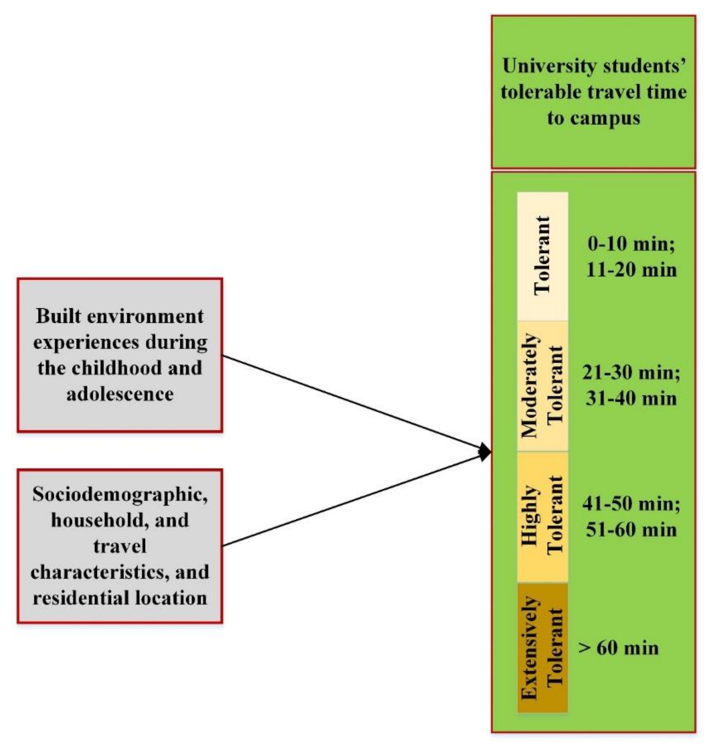
  • What is the most probable TTT of off-campus university students to the campus?
  • To what extent is off-campus university students’ TTT to the campus associated with BE experiences during their childhood and adolescence?
  • How are sociodemographic, household, residential, and travel mode characteristics associated with off-campus university students’ TTT to the campus?
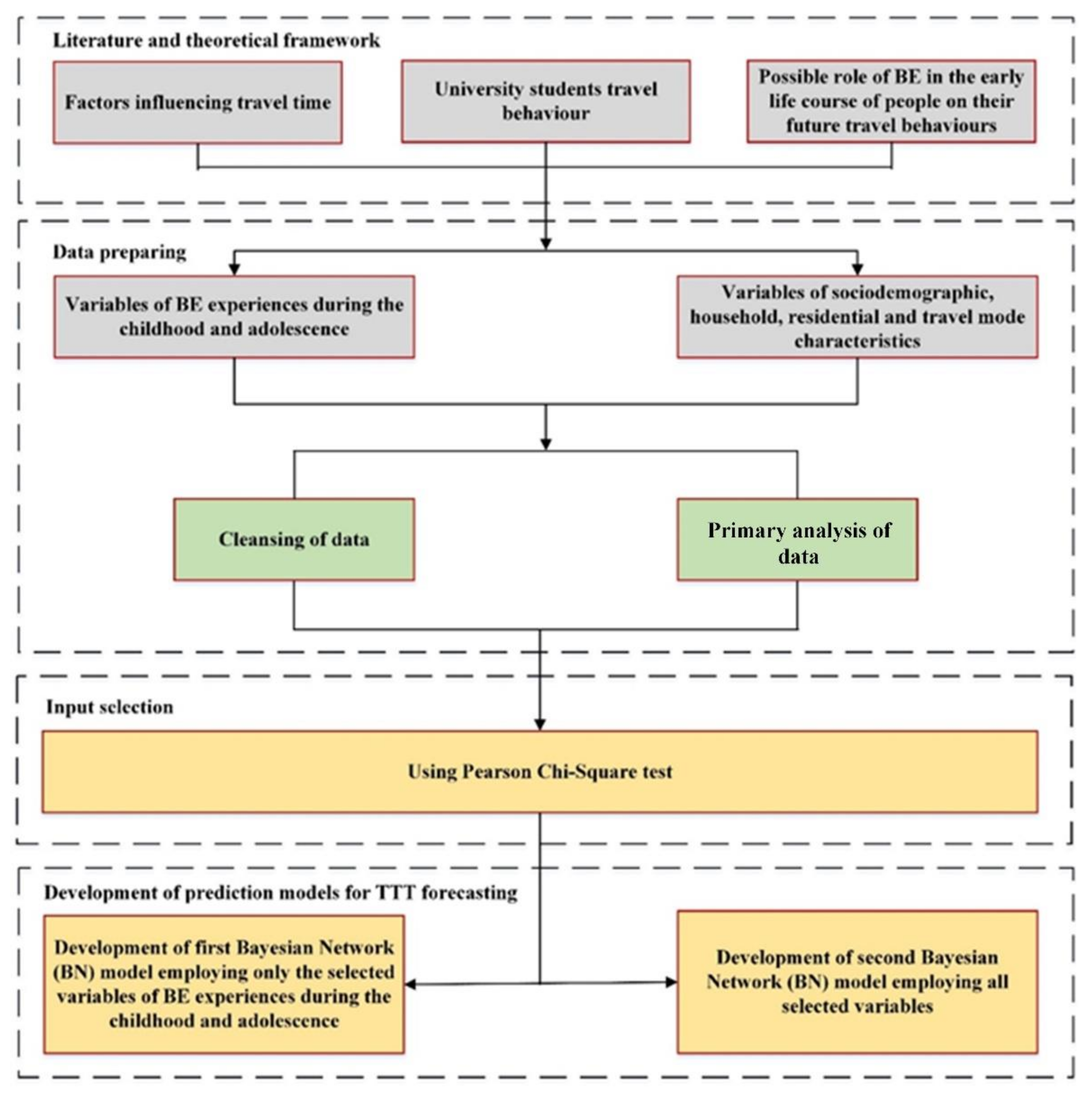
The collection of retrospective data from two universities in Malaysia is used in this study to address these questions using a two-step analysis structure. The details of data collection and analysis are discussed in the subsequent sections.

3. Research Design

This study adopted a retrospective research design. According to Behrens and Mistro [54], this design involves one-time surveys of people and asks participants to remember experiences or events that previously happened to them. The respondents for this present study are off-campus university students that were surveyed and asked to recall their living environments during the age periods of 1–6, 7–13, and 14–18. The retrospective surveys are suitable for observations over long time spans. The literature suggests that the respondents can remember main life-process experiences and can also describe any of their essential characteristics, which enables the assessment of general alternations over more prolonged periods.
This present study evaluated the influence of BE experiences during childhood and adolescence. Using this design, this study thus examined the impact of BE experiences during childhood and adolescence on university students’ TTT to campus. van de Coevering et al. [55] pointed out that the principal disadvantage of the retrospective design is that the examination of opinions and specification of everyday travel behavior are misleading. The authors thus adopted a comparably short time span and urged university students to show preferences for their tolerable travel time on a nominal measure. The survey particularly inquired about current inclinations and regarded these trends as steady throughout university time. The critical role of control variables on the study of BE and travel behavior is undeniable and these variables cannot be eliminated from the modelling procedure [55,56]. Therefore, this study has considered the effects of these variables in the second series of models to obtain a more rigorous research design. The possible effects of different influential factors on university students’ TTT to campus are presented in Figure 1.

3.1. Variables of Built Environment during the Early Life-Course of People

The impact of the built environment on university students’ TTT to campus was investigated through the "5Ds" model. Initially, Cervero and Kockelman [57] developed the "3Ds" model which included density, diversity, and design to express the urban structure. Subsequently, Ewing et al. [58] combined two more dimensions, including destination accessibility and distance to transit, with the previous model and developed the "5Ds" model. The magnitude of land use for residence, work, and other goals is regarded as density. Diversity relates to the level of heterogeneity of land use. The properties of the street network and the walking environment quality are viewed as the design. Distance to transit refers to the accessibility to public transportation facilities. Finally, the measurement of ease of access to trip attractions is referred to as destination accessibility.

3.2. Survey and Data Collection

This present study used an online questionnaire survey in March and May 2020 to collect data regarding the TTT of off-campus university students in Malaysia. In comparison with paper-based questionnaires, the online option is more comfortable to complete by the respondents, without any geographical restrictions. This advantage of the online survey makes it a suitable instrument for studies which try to collect data in multiple locations during times in which movements are restricted (e.g., lockdown and quarantine). The respondents of this study were mainly from two public universities in two renowned tertiary education cities. The universities are A and B (for the sake of the blind review process, the case studies are removed from this manuscript). An email was sent to the students’ email account in each university, which explained the aims of the study. Besides, the research team included the internet address of the questionnaire in the email. A reminder email was also sent to the students every two weeks to increase the response rate and balance the sample size.
The questionnaire comprised three main sections. The initial section examined the respondents’ sociodemographic and household characteristics. The second part involved some questions regarding current residential location and the usual travel mode to the campus. The third part asked students to recall their living environment during two periods of age, namely 7–13 and 14–18. This part also assessed the attitudes of respondents towards their living environment during the mentioned age periods in the form of Likert scale measurement. Once the questionnaire was designed, the research team sent a full version of the questionnaire to a panel of experts, which included urban planners and transport planners. The panel was urged to give their feedback regarding the suitability and communicability of the questionnaire. Likewise, the panel was deemed fit to modify, add, or remove any item from the questionnaire. Minor changes were made to the questionnaire as a result of the experts’ consultation. For instance, the time and distance scales for TTT and tolerable travel distance have become finer to avoid difficulties from the extremely large discretization of travel distance and TT.
Following the panel review, the research team conducted a pilot survey and collected 33 completed questionnaires. The research team also asked the respondents to express any difficulties or incommunicability they found in filling the questionnaire. This pilot survey resulted in some changes in the questionnaire. The main change was made to the age scale. Before the pilot study, the attitudes of the students towards their living environment were supposed to be assessed using three age periods, which are 1–6, 7–13, and 14–18. However, the respondents’ feedback indicated that it was difficult for them to recall their living environment during the age period of 1–6. Besides, the primary analysis result also showed that responses related to this age range were inconsistent. Thus, the age period of 1–6 was removed from the age scale for all survey items, except the question which asked the respondents to indicate the type of settlement (city, village, and suburb) in which they have lived. Age scale of this question has not been changed because it was easy for the respondents to recall general rather than specific characteristics of the living environment. Consequently, the final version of the questionnaire included 49 questions. The questionnaire items that were utilized in this present research are presented in Table 1.

3.3. Analysis Approaches and Techniques

Multiple traditional statistical methods, including the multinomial logit, binary logit, and mixed logit models were frequently employed in studies related to transport for analyzing predictors of the university students’ travel behaviors, particularly their mode choice [59,60,61,62]. The data related to travel behaviors are generally bulky and complicated, which makes the use of regression models challenging for studying predictors of the travel behaviors and patterns. These models typically assume that the associations between the variables are linear and consider the data without outliers [63,64,65]. However, these assumptions are hardly adequate for travel behavior data. Another daunting task, which can occur in regression models, is using the cross-product terms for distinguishing the predictors because of interaction that happens in complicated configurations [66]. Moreover, according to Karlaftis and Golias [67] and Yan, Richards, and Su [66], regression models are often unable to efficiently handle differing categorical variables.
To remedy the above shortcomings of regression models, this study employed non-parametric and machine learning (ML) techniques. These techniques refer to a procedure that makes use of preprocessing, input selection, and extraction and classification processes. The body of literature suggested that ML techniques such as Bayesian network (BN) are free of assumptions of variable distributions; thus, possessing prior probabilistic knowledge on university students’ travel behavior and their TTT is not needed. The ML techniques are also effective in dealing with outliers and many categorical variables. Finally, these techniques efficiently extract knowledge from massive data [68,69,70,71,72,73]. Pearson chi-square test and BN have been successfully applied in a limited number of studies related to transport [74]. However, to the best of the authors’ knowledge, no study has employed both Pearson chi-square test and BN in the study of the university students’ travel behaviors and their TTT.
This present study used a two-step approach to analyze the data collected. The first step was to examine the association between the input variables and the target variable through Pearson chi-square tests. The variables with a value greater than 0.75 were selected as the most associated variables with the target variable and were selected to be used as the inputs of prediction models. Next, two BN models were developed to predict the university students’ TTT to campus. While the first model was applied to those BE variables (during childhood and adolescence) that were selected in the input selection step, the second model was applied to all selected variables. Figure 2 shows the study process and framework.

3.4. Bayesian Network Model

BN is a probabilistic network model that employs the probability theory and the graph system concurrently. The theory behind the BN analysis is the Bayesian probability. The analysis employs joint distributions and preceding distributions of each variable to measure a subsequent distribution for each variable of concern. Two principal parts of BN are probabilistic and graphical structures. A graph K = (H, L) is defined by a collection of nodes H = {H1,…, Hp} and a collection of edges LH × H. In a BN, the nodes H denote the variables, and the edges L signify the directed arrows, showing the conditional dependencies amongst these variables. Equation (1) manifests the probabilistic relationships between the nodes defined by a function of joint probability density F(H).
F H 1 ,   ,   H k = i = 1 k F ( V i | P a r e n t H i ) .  
The conditional probability tables reflect the aforementioned joint likelihood density function, developing the probabilistic BN composition. The BN graphical arrangement necessity possesses an acyclic character. In particular, a BN follows a directed acyclic graph formation. To be precise, there must not be any edge redirecting, including H i   H i for any Hi and H. The edges reveal the mathematical dependencies among the nodes; however, the edge direction may not inevitably indicate a causality association. Between a pair of nodes linked together by an edge, the preceding and following nodes are named parent and child, subsequently. To build the Bayesian networks, this study utilized the Markov blanket, which finds all the variables in the network that are essential to forecast the target variable. A simple structure of BN based on directed acyclic graph formation is shown in Figure 3.
Generally, travel behavior datasets contain various parameters, and each parameter may have diverse classes. Besides, when new knowledge is accessible or needed, these datasets may remain constantly updated. Moreover, it is very common that travel behavior datasets are incomplete or possess missing values. Several studies acknowledged that the BN technique can deal with variables with various classes and undersampling data efficiently. Additionally, this technique can handle data that are deficient, fallacious, or dubious [75,76,77]. According to Tareeq and Inamura [78], the BN technique was considered proper to learn changeable behaviors (including the TTT under review) because it can effectively improve its network following the data specified or inserted into it.
The BN works excellently with a limited number of candidate variables [79]; thus, the Pearson chi-square tests were employed to reduce data dimensionality and select only the most relevant inputs. Pearson chi-square test is a non-parametric statistical test which is applied to sets of categorical data to assess how probable it was that any observed variation between the sets occurred by chance. This test is suitable for feature selection when the target variables of some inputs are categorical. Equation (2) shows the mathematical formulation of the Pearson chi-square test.
χ 2 = A r A e 2 A e
where the Ar and Ae are the real and expected frequencies of categories.

4. Results

This present study created a dataset that included 758 university students’ travel data from two public universities in Malaysia. The dataset contains only the off-campus participants. As previously mentioned, this study aims to predict the tolerable travel time of the university students to the campus considering their past built environment experiences. On the TTT frequencies, 68.35% of students were tolerant, 3.69% were moderately tolerant, 18.99% were highly tolerant, and 8.97% were extensively tolerant. The age range of the majority of students was 19–24 (73.88%). This overrepresentation was believed to have stemmed from the fact that younger students were more capable of and interested in participating in an online survey. Moreover, the older students might be involved in some family matters or might have had less free time, and thus, had much less time for filling in the online questionnaire. The study trends can be extrapolated to other university students because of the size and variety of this study. The sociodemographic characteristics and respondents’ profiles are presented in Appendix A.

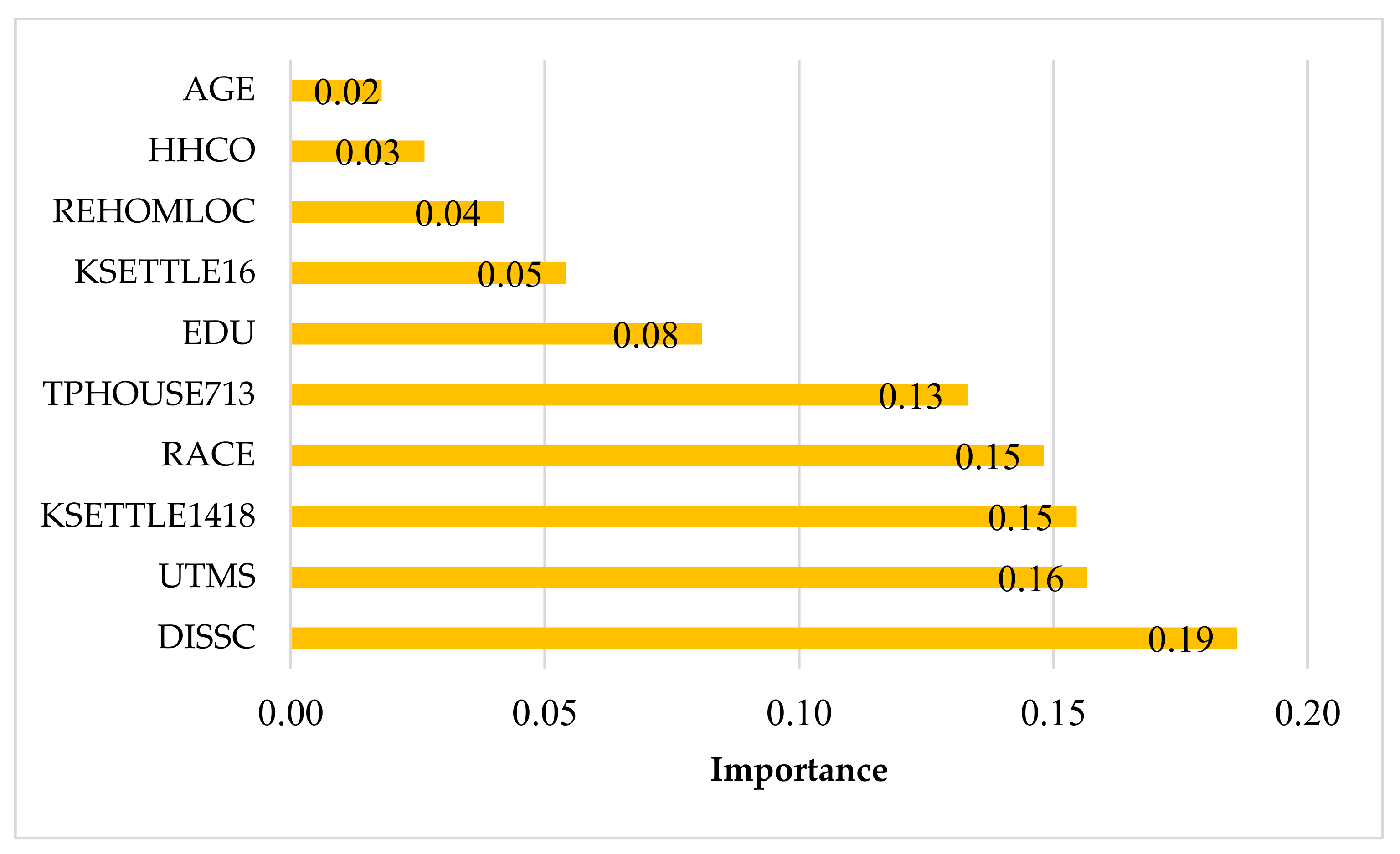
4.1. Input Selection

The associations of 74 input variables with the target variable (TTT to campus) were tested through the Pearson chi-square tests. This present study selected those variables with the value of 0.75 and above as the most associated and important inputs for predicting the students’ TTT to campus. Thus, 38 input variables were selected (Table 2). Furthermore, these variables will be used to develop two predictive BN models. Among the total variables, distance from home to campus (DISSC) was the most important variable, while for variables of BE during the childhood and adolescence of students, the ease of access to the primary/secondary school in the age range of 7–13 (3ACCESSIBILITY713) was the most important variable and was followed by the ease of access to local stores in the same age period (1ACCESSIBILITY713).

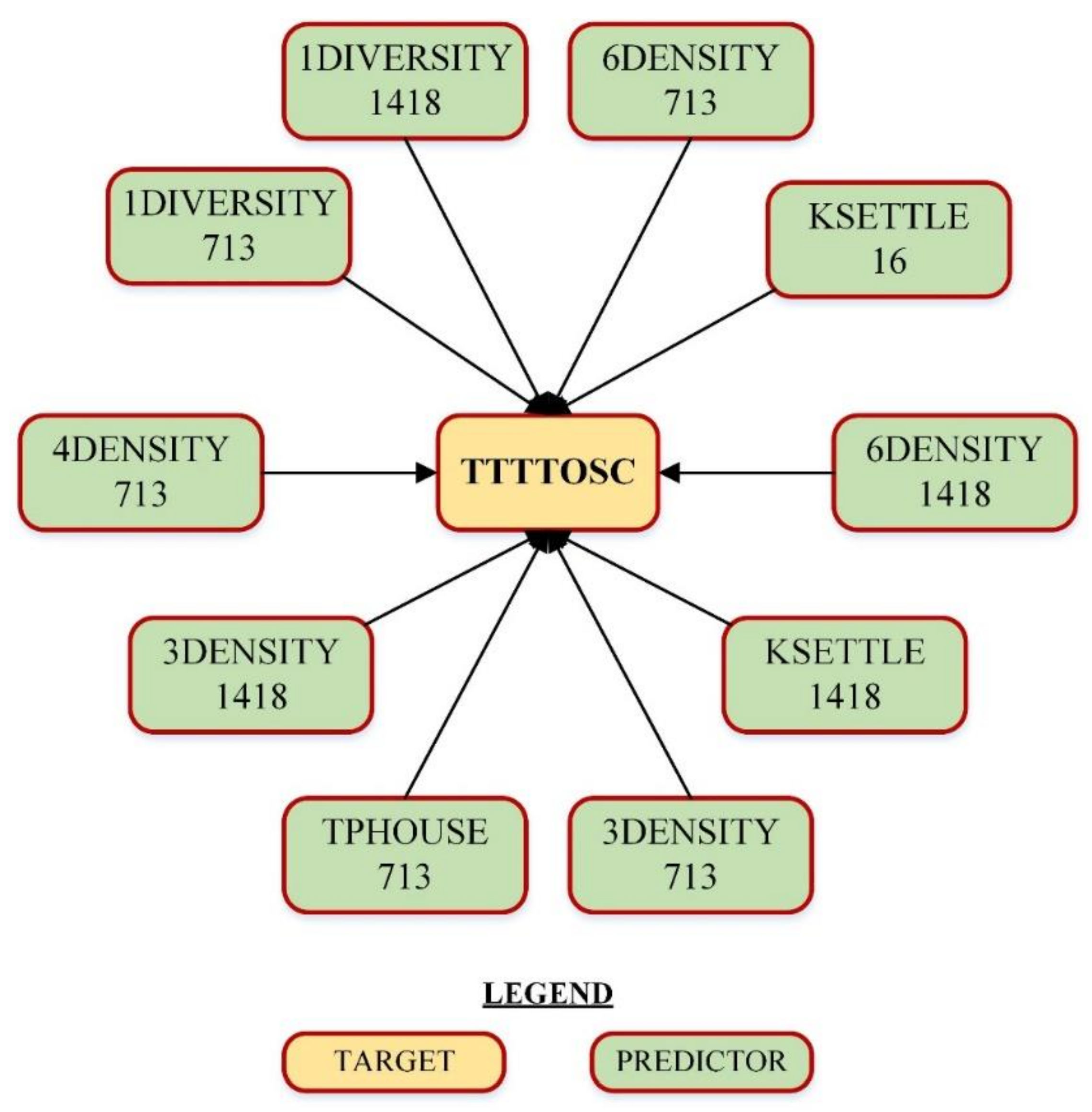
4.2. BN#1 Model Focusing on BE Attributes

The first BN model was developed using 27 BE variables that were chosen in the previous step. This model selected the 10 most important variables to predict the TTT of university students to campus. The training accuracy of this model was 97.47%. The BN#1 structure is presented in Figure 4. This diagram includes 11 variables, 10 predictors, and 1 target variable. The importance of each predictor is shown in Figure 5. As evidently shown, the availability of residential buildings in the neighborhood that respondents lived in, within the age period of 14–18, was the most critical predictor. This predictor was followed by the proximity of the house to shops in the age range of 14–18. The least essential predictor was the type of settlement in the age period of 14–18. As analytically revealed, settlement type in the age range of 1–6 was more critical than 14–18. From the age group perspective, settlement type was the only factor that was assessed by this study for the age range of 1–6. This predictor was selected as an essential predictor by the BN. For the age range of 7–13, four predictors were the most important, which are: (1) availability of residential buildings in the neighborhood, (2) availability of schools in the neighborhood, (3) availability of entertainment facilities in the neighborhood, and (4) proximity of the house to shops. For the age range of 14–18, four predictors were the most important, which are: (1) availability of residential buildings in the neighborhood, (2) availability of schools in the neighborhood, (3) proximity of the house to shops, and (4) settlement type.
The BN#1 identified 76 conditional probabilities for each category of TTT, except TTT of 21–30 min. No TTT of 21–30 min was predicted by BN#1. To simplify the interpretation of the probabilities, only high probable TTTs (probability ≥ 0.75) were reported for each category. The most frequent and influential value of each predictor that predicted each TTT is presented in Table 3.
Figure 6 summarizes the TTTs according to important variables identified by BN#1. This study also calculated the p-value to identify those BE variables that may cause a significant difference in TTTs. Based on the calculations, the significant difference in TTTs was found only in 1DIVERSITY1418 (p-value = 0.011). This means that attitudes of students regarding the availability of shops near their houses during the ages of 14–18 resulted in a significant difference in TTT to campus. Figure 6 shows that students who had shops near their house tended to choose shorter TTTs.

4.3. BN#2 Model Considering the Control Variables and BE Variables

The second BN model was developed using 38 variables. These variables included personal characteristics of the respondents, their household characteristics, variables related to the residential location, and travel mode choice. Eventually, the BN#2 selected 10 predictors as the most important and built the diagram based on these predictors (Figure 7 and Figure 8). The training accuracy of this model was 81.01%. Apparently, among the BE variables, settlement type during the age periods of 1–6 and 14–18, as well as residential/house type during the age period of 7–13 were selected as the most important. Among the controlled variables, age, education level, race, usual travel mode to campus, and distance to campus were chosen as the most important.
The BN#2 identified 53 conditional probabilities for each category of TTT, except TTT of 21–30 min. No TTT of 21–30 min was predicted by BN#2. To simplify the interpretation of the probabilities, only high probable TTTs (probability ≥ 0.75) were reported for each category. The most frequent and influential value of each predictor for predicting each TTT is presented in Table 4.
A summary of TTTs by important control variables is presented in Figure 9. This study assessed whether any significant difference among TTTs exists regarding race, gender, education level, usual travel mode to campus, and distance to campus. Calculations obtained showed that differences in age and distance to campus significantly resulted in different TTTs (p-value = 0.008 and 0.000, respectively). The results indicated that the majority of younger students prefer to choose shorter TTTs. On the other hand, older students were inclined to select longer TTTs, such as 41–50 min. While the majority of students who lived closer to their school chose shorter TTTs, the students who lived far from the school (more than 51 km) selected longer TTTs (more than 60 min). Figure 10 shows principal reasons for selecting the current houses by university students which provide a deeper insight into the factors that influenced university students’ residential choices.

5. Discussion

Cumulatively, 68.33% of university students possessed TTT below 20 min to campus. This finding is in line with those of previous studies that revealed that ideal travel times below 20 min to different destinations were desirable for most of their respondents [80,81,82]. On the other hand, TTT found in this study differ from those described in He, Zhao, and He [30], Milakis and Van Wee [83], and Ye et al. [84], which showed that their participants’ ideal commute time was mostly above 20 min. The possible reason for this contradiction could be the differences between the travel behavior and pattern of university students and other people [20,21].
The BE variables selected by the BN#1 model as the most important indicated that all variables related to the size, type, and composition of BEs may influence the TTT of university students to campus. These variables included those related to the settlement type, neighborhood density and diversity, and residential type. Till date, literature has confirmed the importance of current neighborhood attributes related to density and diversity in establishing the current travel behavior of commuters [85,86,87,88]. However, the results of this study are an immense and creative contribution to the body of literature that confirms that the past living environment experience of students in a diverse BE can affect their future travel behavior, particularly their TTT.
The first and second BN models showed that three BE attributes, including settlement type during the age period of 1–6, settlement type during the age period of 14–18, and apartment/house type during the age period of 7–13, are among the most influential factors of university students’ TTT to campus. By retaining these large-scale BE variables in the BN#2, it can be indicatively explained that size and type attributes of BE may have more impact on the TTT of university students compared to the composition attributes. Moreover, the Pearson correlation tests did not find significant relationships between house type during the age period of 14–18 and the settlement type through the age period of 7–13 and TTT. However, this does not mean that the settlement and house type within these age periods do not influence the TTT of university students. Again, these variables may have less impact compared to peers of other age periods. These findings are unique in the sense that they provide insights into the importance of the role of built environment experiences during childhood and adolescence for analyzing university students’ travel behavior. In addition, to the authors of this study’s best knowledge, this is the first time that the impact of these kinds of experiences on university students’ TTT to campus has been examined.
The BN#2 model did not adopt the BE variables related to diversity and density (which were selected as important variables by BN#1 model), to predict the TTT of university students to campus in the presence of control variables. This implies that a combination of sociodemographic attributes, trip characteristics, and non-composition BE attributes are more efficient variable sets for TTT forecasting of university students to campus. A possible explanation for this may emerge from the ability of people to recall larger characteristics of their living environment during their childhood and adolescence. Indeed, it is quite easy for people to remember the type of house and settlement in which they once lived.
The importance of BE variables for predicting the TTTs varied by age period. For example, for settlement type, the age periods of 1–6 and 14–18 were important while the age period of 7–13 was not. However, it is necessary to remark that this conclusion does not suggest that settlement type in the age period of 7–13 was not important at all but that it was less significant than other age periods for predicting the TTT of university students to campus. For those variables that were important in both the age periods of 7–13 and 14–18 (1DIVERSITY, 6DENSITY, and 3DENSITY), it could be argued that these variables would play a significant role in developing the future students’ travel behavior and constantly affected the development of their travel habits and preferences. Arguably, availability of shops near the respondents’ past houses and availability of residential buildings, entertainment facilities, and schools in the respondents’ past neighborhoods may influence other future travel behaviors of people.
With regards to the controlled variables, race, age, and education level of students were selected as the critical sociodemographic variables to predict the TTT of university students to campus. Additionally, this present study identified the usual travel mode and distance of the school from home as important predictors of TTT of university students. However, no previous studies have assessed the impacts of such variables on TTT of university students. He, Zhao, and He [30] found the significant impacts of age, education level, and travel mode on tolerance threshold of commuting time of the general population to be important variables. Besides, the contribution of sociodemographic factors and travel mode to the TTT of the general population was confirmed in Páez and Whalen [89] and Redmond and Mokhtarian [90].
It was evidently shown that younger students tend to select shorter TTTs to campus. One important reason for this issue is that most survey participants (73.88%) belonged to the age cluster of 19–24 years. This is also in line with the fact that most UM and UTM students are in this age spectrum. Generally, younger students possess a weaker socioeconomic status compared to their older peers. They cannot buy a car and mostly use other active travel modes [91,92]. However, in this study, a majority of the students (73.62%) used private vehicles (car and motorcycle) to travel to campus. This result may be rooted in the high rate of vehicle ownership in Malaysia [93]. At the same time, 7.65% of the students adopted walking and cycling to campus, and their TTTs were 0–10 and 11–20 min. This finding was different from that of Milakis, Cervero, Van Wee, and Maat [23], Milakis and Van Wee [83], and Le et al. [94], that declared that people who walk or cycle had longer ATT than car users. On the other hand, the findings of this study regarding the lower TTTs of car users were in line with the same findings in the literature [23,83,94].
The analytical findings showed that most students who lived closer to the university experienced a shorter TTT. As explained earlier, most respondents were in the age range of 19–24. In Malaysia, many young students study at universities that are far from their hometowns. Besides, the majority of young students in public universities come from families with low socioeconomic status. Thus, these young students cannot afford to buy a house due to its high price, and they consider travel costs and choose to rent homes close to their campuses.
Certain implications for transport researchers and policy makers may be made from this present study. Findings presented in this study showed that the majority of university students had tendencies to experience shorter TTT to campus. Shorter TTTs may lead students to live in residential areas that are close to their campuses. This proximity of housing to the university may be a good opportunity for decision makers to implement sustainable transport solutions and provide sufficient facilities which could encourage students to use the active transport to campuses, such as sidewalks, bike paths, and bus stops. On the other hand, longer TTTs may lead students to live in housing in suburbs. Consequently, the students have to possess cars or motorcycles for travelling between the campus and residential areas if sufficient public transports are not available. Thus, the university decision makers should consider provision of a sufficient number of cheap housing units near the university campuses to decrease the need for using the private vehicles.
The findings of this present study also indicate that there is substantial homogeneity in the intrinsic preference for different TTTs and past BE experiences may create reference points for future travel behaviors and TTT of individuals. The findings also confirmed the undeniable intervention of BE in people’s travel behaviors. Although using these factors for predicting future travel behaviors is still in its early stages, thus, urban and transport planners should include retrospective questions in their surveys to produce more accurate forecasts. Besides, researchers and policymakers should use longitudinal BE data and track the changes of BE over time and examine possible effects of these changes on individuals’ future travel behaviors.

Limitations

In this present study, reference should be made to several limitations. First, university students may not represent the travel behavior of the general population in Malaysia. Thus, future studies can apply the same approach to different population groups to identify the impacts of the BE experiences during childhood or adolescence on their current travel behaviors. Second, this paper did not capture the TTTs of university students for leisure and shopping trips. Third, the study oversampled participants that have accessed the internet during the lockdown of COVID-19. The fourth constraining point of this study is that our study utilized self-report data. Trip observations may complement the self-report data in future investigations. This study obtained acceptable precision for BN models. However, larger datasets can be employed by further investigations to achieve greater accuracy. Fifthly, the participants of this survey were university students in Malaysia. However, in this country, the rate of vehicle ownership is very high. In addition, the overall condition of infrastructure supporting active transportation is poor. Therefore, the results of this study should be applied with caution to developed countries. Sixthly, this study considered a wide range of BE and sociodemographic factors; however, variables related to perceptions and habits were not included in this study. Thus, future studies can design surveys that include more variables to predict the TTT. Finally, the authors did not assess the BE experiences during the ages of 1-6 because it was challenging for students to remember the BE experiences. Thus, future studies can also include parents in their survey and ask them about the BE conditions when their child was 1–6 years old.

6. Conclusions

This present study used the Pearson chi-square technique and Bayesian network analysis to: (1) determine the most probable TTT of the off-campus university students to the campus; (2) investigate the association between off-campus university students’ TTT to the campus and BE experiences during their childhood and teenage years; and (3) investigate the association between sociodemographic, household, residential, and travel mode characteristics of the off-campus university students’ TTT to the campus.
A retrospective approach was adopted, which considered BE variables in the childhood and adolescent age periods to accompany sociodemographic, household characteristics, and current travel mode choice and residential location. The Pearson chi-square analysis identified 34 variables out of 74 candidate inputs. These variables were involved as predictors of the target (i.e., university students’ TTT to campus) in BN analysis. Two BN models, including BN#1 and BN#2, were developed. The BN#1 applied only on BE variables. By developing this model, the availability of residential buildings in the neighborhoods that respondents lived in, during the age period of 14–18, was shown to be the most critical predictor of TTT of university students to campus. BN#2 was applied on all 34 variables. By running this second model, distance to campus was chosen as the most important. BE variables, including settlement type during the age period of 1–6 and 14–18 and house type in the age period of 7–13, were also identified as the most significant factors.
It is a challenging task to obtain information regarding the past living environment of university students and predict their future travel behavior based on these experiences. However, the results of this study can be instructive for urban and transport planners in the sense that built environment attributes can play an essential role during the whole life-course and the development of travel behaviors and patterns of individuals. To achieve more sustainable commute behavior in the future, planners and designers should consider more compact and mixed-use neighborhoods. In Malaysia, the rate of vehicle ownership is high. While several other factors, such as weather, low price of cars, and cheap parking are associated with this high vehicle ownership rate, advocating more sustainable behaviors may help the youths to minimize the usage of cars. Compact and dense living environments during the early life-course of people may be a desirable setting to shape their future habits. The authors of this study believe that the tendency of people to have shorter TTT could emerge from their experiences of previous living environments, especially during childhood and adolescence. Additionally, experiencing shorter trip distances before adulthood might mean habituation to the higher usage of alternative modes such as public transport, walking, and cycling. During adulthood, the habits of using these modes may result in less flexibility and prevent people from dwelling in suburbs, as well as prevention from sprawling.

Author Contributions

Conceptualization, M.A. (Mahdi Aghaabbasi); formal analysis, M.A. (Mahdi Aghaabbasi); funding acquisition, Y.C., S.A., L.S., S.C., K.N., E.S. and R.F.; investigation, M.A. (Mahdi Aghaabbasi); methodology, M.A. (Mahdi Aghaabbasi); resources, Y.C., M.A. (Mujahid Ali), S.A., L.S., S.C., K.N., E.S., R.F. and R.Z.; supervision, R.Z.; writing—original draft, M.A. (Mahdi Aghaabbasi) and M.A. (Mujahid Ali). All authors have read and agreed to the published version of the manuscript.

Funding

The research is partially funded by the Ministry of Science and Higher Education of the Russian Federation under the strategic academic leadership program “Priority 2030” (Agreement 075-15-2021-1333 dated 30 September 2021).

Acknowledgments

This research is also supported by the National Natural Science Foundation, an Empirical Study on the Protection and Development of Traditional Villages in Minority Areas and Its Modern Spatial Transformation (project approval No.: 51978250). Furthermore, the study was carried out using the equipment of interregional multispeciality and interdisciplinary center for the collective usage of promising and competitive technologies in the areas of development and aplication in industry/mechanical engineering of domestic achievements in the field of nanotechnology (Vladimir State University).

Conflicts of Interest

The authors declare no conflict of interest.

Appendix A

Table A1. Sociodemographic and household characteristics of respondents by their TTT.
Tolerability of Travel Time
TolerateModerate TolerateHighly TolerateExtensively Tolerate
N%N%N%N%
Age
19–2439275.7281008559.05580.9
25–30356.8 149.7
31–367213.9
37–42193.7 1319.1
43–48 2517.4
More than 48 2013.9
Gender
Male29556.9281005638.94160.3
Female22343.1 8861.12739.7
Education level
Primary
Secondary448.51450
Diploma224.2
Bachelor’s degree34867.214509968.85580.9
Master’s degree132.5 2517.41319.1
Doctorate degree9117.6 2013.9
Income
Less than MYR 10009718.7517.93524.31420.6
Between MYR 1000 and MYR 20005811.2414.32013.968.8
Between MYR 2000 and MYR 30007414.3621.41812.5913.2
Between MYR 3000 and MYR 60008917.2414.31812.51116.2
Between MYR 6000 and MYR 13,00014528.0517.94128.52232.4
More than MYR 13,0005510.6414.3128.368.8
Race
Malay26951.9281004833.35479.4
Chinese17333.4 3121.51420.6
Indian142.7 4531.3
Foreigner6212.0 2013.9
Vehicle ownership
Yes5479.41450.08055.6
No1420.61450.06444.468100
Vehicle count
091.713.621.434.4
112924.9621.43121.51420.6
214528.01035.74430.62130.9
>323547.11139.36746.63044.1
Number of children
035167.81760.79062.54769.1
17113.7725.02819.41014.7
25911.4310.7139.068.8
>3377.213.6139.057.4
Number of people in household
140.813.610.722.9
2428.127.1128.345.9
37213.9414.32718.81014.7
>440077.22175.110472.35276.4

References

  1. Wheatley, D. Travel-to-work and subjective well-being: A study of UK dual career households. J. Transp. Geogr. 2014, 39, 187–196. [Google Scholar] [CrossRef] [Green Version]
  2. Ye, R.; Titheridge, H. Impact of Individuals’ Commuting Trips on Subjective Well-Being-Evidence from Xi’an, China; University College London: London, UK, 2015. [Google Scholar]
  3. Oliveira, R.; Moura, K.; Viana, J.; Tigre, R.; Sampaio, B. Commute duration and health: Empirical evidence from Brazil. Transp. Res. Part A Policy Pract. 2015, 80, 62–75. [Google Scholar] [CrossRef]
  4. Ali, M.; Dharmowijoyo, D.B.E.; de Azevedo, A.R.G.; Fediuk, R.; Ahmad, H.; Salah, B. Time-Use and Spatio-Temporal Variables Influence on Physical Activity Intensity, Physical and Social Health of Travelers. Sustainability 2021, 13, 12226. [Google Scholar] [CrossRef]
  5. Ali, M.; Dharmowijoyo, D.B.; Harahap, I.S.; Puri, A.; Tanjung, L.E. Travel behaviour and health: Interaction of Activity-Travel Pattern, Travel Parameter and Physical Intensity. Solid State Technol. 2020, 63, 4026–4039. [Google Scholar]
  6. Dijst, M.; Vidakovic, V. Travel time ratio: The key factor of spatial reach. Transportation 2000, 27, 179–199. [Google Scholar] [CrossRef]
  7. Schwanen, T.; Dijst, M. Travel-time ratios for visits to the workplace: The relationship between commuting time and work duration. Transp. Res. Part A Policy Pract. 2002, 36, 573–592. [Google Scholar] [CrossRef]
  8. Deka, D. The living, moving and travel behaviour of the growing American solo: Implications for cities. Urban Stud. 2014, 51, 634–654. [Google Scholar] [CrossRef]
  9. Bolte, G.; Fromme, H.; Grp, G.M.E.S. Influence of Built Environment and Socioeconomic Position on Children’s Physical Activity During Leisure Time and due to Mode of Travel. Epidemiology 2009, 20, S53. [Google Scholar] [CrossRef]
  10. Ma, X.L.; Yang, J.; Ding, C.; Liu, J.F.; Zhu, Q. Joint Analysis of the Commuting Departure Time and Travel Mode Choice: Role of the Built Environment. J. Adv. Transp. 2018, 2018, 4540832. [Google Scholar] [CrossRef]
  11. Manville, M. Travel and the Built Environment: Time for Change. J. Am. Plan. Assoc. 2017, 83, 29–32. [Google Scholar] [CrossRef]
  12. Molina-Garcia, J.; Menescardi, C.; Estevan, I.; Martinez-Bello, V.; Queralt, A. Neighborhood Built Environment and Socioeconomic Status are Associated with Active Commuting and Sedentary Behavior, but not with Leisure-Time Physical Activity, in University Students. Int. J. Environ. Res. Public Health 2019, 16, 3176. [Google Scholar] [CrossRef] [Green Version]
  13. Mouratidis, K. Built environment and leisure satisfaction: The role of commute time, social interaction, and active travel. J. Transp. Geogr. 2019, 80, 102491. [Google Scholar] [CrossRef]
  14. Yu, L.; Xie, B.L.; Chan, E.H.W. Exploring impacts of the built environment on transit travel: Distance, time and mode choice, for urban villages in Shenzhen, China. Transp. Res. Part E-Logist. Transp. Rev. 2019, 132, 57–71. [Google Scholar] [CrossRef]
  15. Wang, D.; Liu, Y. Factors influencing public transport use: A study of university commuters’ travel and mode choice behaviours. In Proceedings of the State of Australian Cities Conference, Gold Coast, Australia, 9–11 December 2015. [Google Scholar]
  16. Abdul Sukora, N.S.; Hassan, S.A. En route to a sustainable campus–an analysis of university students’ travel patterns via 7 day travel diary. J. Teknol. 2014, 70, 9–16. [Google Scholar] [CrossRef] [Green Version]
  17. Lundberg, B.; Weber, J. Non-motorized transport and university populations: An analysis of connectivity and network perceptions. J. Transp. Geogr. 2014, 39, 165–178. [Google Scholar] [CrossRef]
  18. Whalen, K.E.; Páez, A.; Carrasco, J.A. Mode choice of university students commuting to school and the role of active travel. J. Transp. Geogr. 2013, 31, 132–142. [Google Scholar] [CrossRef]
  19. Aghaabbasi, M.; Shekari, Z.A.; Shah, M.Z.; Olakunle, O.; Armaghani, D.J.; Moeinaddini, M. Predicting the use frequency of ride-sourcing by off-campus university students through random forest and Bayesian network techniques. Transp. Res. Part A Policy Pract. 2020, 136, 262–281. [Google Scholar] [CrossRef]
  20. Garikapati, V.M.; You, D.; Pendyala, R.M.; Patel, T.; Kottommannil, J.; Sussman, A. Design, development, and implementation of a university travel demand modeling framework. J. Transp. Res. Board 2016, 2563, 105–113. [Google Scholar] [CrossRef]
  21. Khattak, A.; Wang, X.; Son, S.; Agnello, P. Travel by university students in Virginia. J. Transp. Res. Board 2011, 2255, 137–145. [Google Scholar] [CrossRef]
  22. Namgung, M.; Akar, G. Influences of neighborhood characteristics and personal attitudes on university commuters’ public transit use. J. Transp. Res. Board 2015, 2500, 93–101. [Google Scholar] [CrossRef]
  23. Milakis, D.; Cervero, R.; Van Wee, B.; Maat, K. Do people consider an acceptable travel time? Evidence from Berkeley, CA. J. Transp. Geogr. 2015, 44, 76–86. [Google Scholar] [CrossRef]
  24. Simon, H.A. Rational choice and the structure of the environment. Psychol. Rev. 1956, 63, 129. [Google Scholar] [CrossRef] [Green Version]
  25. Simon, H.A. A behavioral model of rational choice. Q. J. Econ. 1955, 69, 99–118. [Google Scholar] [CrossRef]
  26. Wright, P.; Barbour, F. Phased Decision Strategies: Sequels to an Initial Screening; Graduate School of Business, Stanford University: Stanford, CA, USA, 1977. [Google Scholar]
  27. Ryan, J.; Zahavi, Y. Stability of Travel Components Over Time. Transp. Res. Rec. 1980, 750, 19–26. [Google Scholar]
  28. Zahavi, Y.; Talvitie, A. Regularities in Travel Time and Money Expenditures. In Proceedings of the 59th Annual Meeting of the Transportation Research Board, Washington, DC, USA, 21–25 January 1980. [Google Scholar]
  29. Mokhtarian, P.L.; Salomon, I. How derived is the demand for travel? Some conceptual and measurement considerations. Transp. Res. Part A Policy Pract. 2001, 35, 695–719. [Google Scholar] [CrossRef] [Green Version]
  30. He, M.; Zhao, S.; He, M. Tolerance threshold of commuting time: Evidence from Kunming, China. J. Transp. Geogr. 2016, 57, 1–7. [Google Scholar] [CrossRef]
  31. Marchetti, C. Anthropological invariants in travel behavior. Technol. Forecast. Soc. Chang. 1994, 47, 75–88. [Google Scholar] [CrossRef] [Green Version]
  32. Wener, R.E.; Evans, G.W.; Phillips, D.; Nadler, N. Running for the 7: 45: The effects of public transit improvements on commuter stress. Transportation 2003, 30, 203–220. [Google Scholar] [CrossRef]
  33. Evans, G.W.; Wener, R.E. Rail commuting duration and passenger stress. Health Psychol. 2006, 25, 408. [Google Scholar] [CrossRef] [Green Version]
  34. Novaco, R.W.; Gonzalez, O.I. Commuting and well-being. In Technology and Psychological Well-Being; Amichai-Hamburger, Y., Ed.; Cambridge University Press: Cambridge, UK, 2009; pp. 174–205. [Google Scholar]
  35. Young, W.; Morris, J. Evaluation by individuals of their travel time to work. Econometrica 1978, 46, 403–426. [Google Scholar]
  36. Hupkes, G. The law of constant travel time and trip-rates. Futures 1982, 14, 38–46. [Google Scholar] [CrossRef]
  37. Ali, M.; de Azevedo, A.R.G.; Marvila, M.T.; Khan, M.I.; Memon, A.M.; Masood, F.; Almahbashi, N.M.; Shad, M.K.; Khan, M.A.; Fediuk, R.; et al. The Influence of COVID-19-Induced Daily Activities on Health Parameters—A Case Study in Malaysia. Sustainability 2021, 13, 7465. [Google Scholar] [CrossRef]
  38. Clark, B.; Chatterjee, K.; Melia, S. Changes to commute mode: The role of life events, spatial context and environmental attitude. Transp. Res. Part A Policy Pract. 2016, 89, 89–105. [Google Scholar] [CrossRef] [Green Version]
  39. Verplanken, B.; Walker, I.; Davis, A.; Jurasek, M. Context change and travel mode choice: Combining the habit discontinuity and self-activation hypotheses. J. Environ. Psychol. 2008, 28, 121–127. [Google Scholar] [CrossRef]
  40. Gao, K.; Yang, Y.; Sun, L.; Qu, X. Revealing psychological inertia in mode shift behavior and its quantitative influences on commuting trips. Transp. Res. Part F Traffic Psychol. Behav. 2020, 71, 272–287. [Google Scholar] [CrossRef]
  41. Lanzendorf, M. Mobility biographies: A new perspective for understanding travel behaviour. In Proceedings of the 10th International Conference on Travel Behaviour Research, Lucerne, Switzerland, 10–15 August 2003. [Google Scholar]
  42. Scheiner, J. Gendered key events in the life course: Effects on changes in travel mode choice over time. J. Transp. Geogr. 2014, 37, 47–60. [Google Scholar] [CrossRef]
  43. Lanzendorf, M. Key events and their effect on mobility biographies: The case of childbirth. Int. J. Sustain. Transp. 2010, 4, 272–292. [Google Scholar] [CrossRef]
  44. Van der Waerden, P. The influence of key events and critical incidents on transport mode choice switching behaviour: A descriptive analysis. In Proceedings of the Proceedings of 10th International Conference on Travel Behaviour Research, Lucerne, Switzerland, 10–15 August 2003. [Google Scholar]
  45. Clark, B.; Chatterjee, K.; Melia, S.; Knies, G.; Laurie, H. Life events and travel behavior: Exploring the interrelationship using UK household longitudinal study data. Transp. Res. Rec. 2014, 2413, 54–64. [Google Scholar] [CrossRef] [Green Version]
  46. Scheiner, J.; Holz-Rau, C. Changes in travel mode use after residential relocation: A contribution to mobility biographies. Transportation 2013, 40, 431–458. [Google Scholar] [CrossRef]
  47. González, R.M.; Marrero, Á.S.; Cherchi, E. Testing for inertia effect when a new tram is implemented. Transp. Res. Part A Policy Pract. 2017, 98, 150–159. [Google Scholar] [CrossRef] [Green Version]
  48. Yeh, A.G.; Yuen, B. Tall building living in high density cities: A comparison of Hong Kong and Singapore. In High-Rise Living in Asian Cities; Springer: Berlin/Heidelberg, Germany, 2011; pp. 9–23. [Google Scholar]
  49. Yeh, A.G.-O. The Planning and Management of a Better High Density Environment; Routledge: London, UK, 2000; p. 400. [Google Scholar]
  50. Takayama, N.; Petrova, E.; Matsushima, H.; Furuya, K.; Ueda, H.; Mironov, Y.; Petrova, A.; Aoki, Y. Values, Concerns, and Attitudes Toward the Environment in Japan and Russia. Urban Reg. Plan. Rev. 2015, 2, 43–67. [Google Scholar] [CrossRef] [Green Version]
  51. Deiner, P. Inclusive Early Childhood Education: Development, Resources, and Practice; Cengage Learning: Boston, MA, USA, 2012. [Google Scholar]
  52. Michael Page. How Long Is Your Commute to Work? Available online: https://www.michaelpage.com.my/content/how-long-is-your-commute-to-work/ (accessed on 1 January 2020).
  53. Mbara, T.C.; Celliers, C. Travel patterns and challenges experienced by University of Johannesburg off-campus students. J. Transp. Supply Chain. Manag. 2013, 7, 167700576. [Google Scholar] [CrossRef]
  54. Behrens, R.; Mistro, R.D. Shocking habits: Methodological issues in analyzing changing personal travel behavior over time. Int. J. Sustain. Transp. 2010, 4, 253–271. [Google Scholar] [CrossRef]
  55. van de Coevering, P.; Maat, K.; van Wee, B. Multi-period Research Designs for Identifying Causal Effects of Built Environment Characteristics on Travel Behaviour. Transp. Rev. 2015, 35, 512–532. [Google Scholar] [CrossRef]
  56. de Azevedo, A.R.G.; Marvila, M.T.; Ali, M.; Khan, M.I.; Masood, F.; Vieira, C.M.F. Effect of the addition and processing of glass polishing waste on the durability of geopolymeric mortars. Case Stud. Constr. Mater. 2021, 15, e00662. [Google Scholar] [CrossRef]
  57. Cervero, R.; Kockelman, K. Travel demand and the 3Ds: Density, diversity, and design. Transp. Research. Part D Transp. Environ. 1997, 2, 199–219. [Google Scholar] [CrossRef]
  58. Ewing, R.; Greenwald, M.; Zhang, M.; Walters, J.; Feldman, M.; Cervero, R.; Thomas, J. Measuring the Impact of Urban form and Transit Access on Mixed Use Site Trip Generation Rates—Portland Pilot Study; US Environmental Protection Agency: Washington, DC, USA, 2009.
  59. Rotaris, L.; Danielis, R.; Maltese, I. Carsharing use by college students: The case of Milan and Rome. Transp. Res. Part A Policy Pract. 2019, 120, 239–251. [Google Scholar] [CrossRef]
  60. Nguyen-Phuoc, D.Q.; Amoh-Gyimah, R.; Tran, A.T.P.; Phan, C.T. Mode choice among university students to school in Danang, Vietnam. Travel Behav. Soc. 2018, 13, 1–10. [Google Scholar] [CrossRef]
  61. Tezcan, H.O. Potential of carpooling among unfamiliar users: Case of undergraduate students at Istanbul Technical University. J. Urban Plan. Dev. 2016, 142, 04015006. [Google Scholar] [CrossRef]
  62. Zhou, J. Proactive sustainable university transportation: Marginal effects, intrinsic values, and university students’ mode choice. Int. J. Sustain. Transp. 2016, 10, 815–824. [Google Scholar] [CrossRef]
  63. Stylianou, K.; Dimitriou, L.; Abdel-Aty, M. Big data and road safety: A comprehensive review. In Mobility Patterns, Big Data and Transport Analytics; Elsevier: Amsterdam, The Netherlands, 2019; pp. 297–343. [Google Scholar]
  64. Ali, M.; Room, S.; Khan, M.I.; Masood, F.; Ali Memon, R.; Khan, R.; Memon, A.M. Assessment of local earthen bricks in perspective of physical and mechanical properties using Geographical Information System in Peshawar, Pakistan. Structures 2020, 28, 2549–2561. [Google Scholar] [CrossRef]
  65. Lv, Z.; Li, Y.; Feng, H.; Lv, H. Deep Learning for Security in Digital Twins of Cooperative Intelligent Transportation Systems. IEEE Trans. Intell. Transp. Syst. 2021, 22, 1–10. [Google Scholar] [CrossRef]
  66. Yan, X.; Richards, S.; Su, X. Using hierarchical tree-based regression model to predict train-vehicle crashes at passive highway-rail grade crossings. Accid. Anal. Prev. 2010, 42, 64–74. [Google Scholar] [CrossRef] [PubMed]
  67. Karlaftis, M.G.; Golias, I. Effects of road geometry and traffic volumes on rural roadway accident rates. Accid. Anal. Prev. 2002, 34, 357–365. [Google Scholar] [CrossRef]
  68. Ahmad, I.; Basheri, M.; Iqbal, M.J.; Rahim, A. Performance comparison of support vector machine, random forest, and extreme learning machine for intrusion detection. IEEE Access 2018, 6, 33789–33795. [Google Scholar] [CrossRef]
  69. Utkin, L.V.; Konstantinov, A.V.; Chukanov, V.S.; Kots, M.V.; Ryabinin, M.A.; Meldo, A.A. A weighted random survival forest. Knowl.-Based Syst. 2019, 177, 136–144. [Google Scholar] [CrossRef] [Green Version]
  70. Khatami, A.; Khosravi, A.; Nguyen, T.; Lim, C.P.; Nahavandi, S. Medical image analysis using wavelet transform and deep belief networks. Expert Syst. Appl. 2017, 86, 190–198. [Google Scholar] [CrossRef]
  71. Friedman, N.; Geiger, D.; Goldszmidt, M. Bayesian Network Classifiers. Mach. Learn. 1997, 29, 131–163. [Google Scholar] [CrossRef] [Green Version]
  72. Barreto, E.D.; Stafanato, K.V.; Marvila, M.T.; de Azevedo, A.R.; Ali, M.; Pereira, R.M.; Monteiro, S.N. Clay Ceramic Waste as Pozzolan Constituent in Cement for Structural Concrete. Materials 2021, 14, 2917. [Google Scholar] [CrossRef]
  73. Qian, Y.; Aghaabbasi, M.; Ali, M.; Alqurashi, M.; Salah, B.; Zainol, R.; Moeinaddini, M.; Hussein, E.E. Classification of Imbalanced Travel Mode Choice to Work Data Using Adjustable SVM Model. Appl. Sci. 2021, 11, 11916. [Google Scholar] [CrossRef]
  74. Leilabadi, S.H.; Schmidt, S. In-depth Analysis of Autonomous Vehicle Collisions in California. In Proceedings of the 2019 IEEE Intelligent Transportation Systems Conference (ITSC), Auckland, NZ, USA, 27–29 October 2019. [Google Scholar]
  75. Liu, T.; Zhang, Y.; Chen, J.; Shen, H. Discovery of Association Rule of Learning Action Based on Bayesian Network. In Proceedings of the 2018 9th International Conference on Information Technology in Medicine and Education (ITME), Hangzhou, China, 19–21 October 2018; pp. 466–470. [Google Scholar]
  76. Susanti, S.P.; Azizah, F.N. Imputation of missing value using dynamic Bayesian network for multivariate time series data. In Proceedings of the 2017 International Conference on Data and Software Engineering (ICoDSE), Buenos Aires, Argentina, 20–28 May 2017; pp. 1–5. [Google Scholar]
  77. Wu, Q.; Yang, C.; Gao, X.; He, P.; Chen, G. EPAB: Early Pattern Aware Bayesian Model for Social Content Popularity Prediction. In Proceedings of the 2018 IEEE International Conference on Data Mining (ICDM), Singapore, 17–20 November 2018; pp. 1296–1301. [Google Scholar]
  78. Tareeq, S.M.; Inamura, T. A sample discarding strategy for rapid adaptation to new situation based on Bayesian behavior learning. In Proceedings of the 2008 IEEE International Conference on Robotics and Biomimetics, Bangkok, Thailand, 14–17 December 2009; pp. 1950–1955. [Google Scholar]
  79. Prati, G.; Pietrantoni, L.; Fraboni, F. Using data mining techniques to predict the severity of bicycle crashes. Accid. Anal. Prev. 2017, 101, 44–54. [Google Scholar] [CrossRef] [PubMed]
  80. O’Fallon, C.; Wallis, I. A Wider Look at How Travellers Value the Quality and Quantity of Travel Time; NZ Transport Agency Research Report 469; NZ Transport Agency: Wellington, New Zealand, 2012; p. 128.
  81. Russell, M.L. Travel Time Use on Public Transport: What Passengers Do and How It Affects Their Wellbeing; University of Otago: Dunedin, New Zealand, 2012. [Google Scholar]
  82. Russell, M.; Mokhtarian, P. How real is a reported desire to travel for its own sake? Exploring the ‘teleportation’ concept in travel behaviour research. Transportation 2014, 42, 333–345. [Google Scholar] [CrossRef]
  83. Milakis, D.; Van Wee, B. “For me it is always like half an hour”: Exploring the acceptable travel time concept in the US and European contexts. Transp. Policy 2018, 64, 113–122. [Google Scholar] [CrossRef]
  84. Ye, R.; De Vos, J.; Ma, L. Analysing the association of dissonance between actual and ideal commute time and commute satisfaction. Transp. Res. Part A Policy Pract. 2020, 132, 47–60. [Google Scholar] [CrossRef]
  85. Ewing, R.; Cervero, R. Travel and the built environment. J. Am. Plan. Assoc. 2010, 76, 265–294. [Google Scholar] [CrossRef]
  86. Cervero, R. Built environments and mode choice: Toward a normative framework. Transp. Res. Part D Transp. Environ. 2002, 7, 265–284. [Google Scholar] [CrossRef]
  87. Cervero, R.; Duncan, M. Walking, bicycling, and urban landscapes: Evidence from the San Francisco Bay Area. Am. J. Public Health 2003, 93, 1478–1483. [Google Scholar] [CrossRef] [PubMed]
  88. Ewing, R.; Handy, S. Measuring the unmeasurable: Urban design qualities related to walkability. J. Urban Des. 2009, 14, 65–84. [Google Scholar] [CrossRef]
  89. Páez, A.; Whalen, K. Enjoyment of commute: A comparison of different transportation modes. Transp. Res. Part A Policy Pract. 2010, 44, 537–549. [Google Scholar] [CrossRef]
  90. Redmond, L.S.; Mokhtarian, P.L. The positive utility of the commute: Modeling ideal commute time and relative desired commute amount. Transportation 2001, 28, 179–205. [Google Scholar] [CrossRef]
  91. Habib, K.N.; Weiss, A.; Hasnine, S. On the heterogeneity and substitution patterns in mobility tool ownership choices of post-secondary students: The case of Toronto. Transp. Res. Part A Policy Pract. 2018, 116, 650–665. [Google Scholar] [CrossRef]
  92. Mitra, R.; Nash, S. Can the built environment explain gender gap in cycling? An exploration of university students’ travel behavior in Toronto, Canada. Int. J. Sustain. Transp. 2018, 13, 138–147. [Google Scholar] [CrossRef]
  93. Govindaraju, V.C. Greening the economy with low carbon energy system: Developments, policy initiatives and lessons from Malaysia. In Investing on Low-Carbon Energy Systems; Springer: Berlin/Heidelberg, Germany, 2016; pp. 111–129. [Google Scholar]
  94. Le, H.T.K.; Buehler, R.; Fan, Y.; Hankey, S. Expanding the positive utility of travel through weeklong tracking: Within-person and multi-environment variability of ideal travel time. J. Transp. Geogr. 2020, 84, 102679. [Google Scholar] [CrossRef]
Figure 1. Schematic diagram of possible factors influencing university students’ tolerable travel time to campus and the classifications of tolerable travel time used in this study.
Sustainability 14 00325 g001
Figure 2. The framework of this study.
Sustainability 14 00325 g002
Figure 3. Simple BN network.
Sustainability 14 00325 g003
Figure 4. BN diagram to predict the TTT of university students to campus considering only the effects of BE variables.
Sustainability 14 00325 g004
Figure 5. Importance of 14 variables to predict the TTT of students to campus considering only the BE features.
Sustainability 14 00325 g005
Figure 6. Histograms of TTT to school by important predictors of BN#1.
Sustainability 14 00325 g006aSustainability 14 00325 g006b
Figure 7. BN#2 diagram to predict the TTT of university students to campus considering the effects of control variables and the BE variables.
Sustainability 14 00325 g007
Figure 8. Importance of variables to predict the TTT of students to campus considering the effects of control variables and BE variables.
Sustainability 14 00325 g008
Figure 9. Histograms of TTT to campus by important control predictors of BN#2.
Sustainability 14 00325 g009
Figure 10. Top reasons to choose the residential location by the university students.
Sustainability 14 00325 g010
Table 1. Variables employed in this study.
VariableDescriptionValue
Sociodemographic and household characteristics
AGERespondent’s age(1) 19–24; (2) 25–30; (3) 31–36; (4) 37–42; (5) 43–48; (6) more than 48
GENRespondent’s gender(1) male; (2) female
EDUHighest education level of respondent(1) primary; (2) secondary; (3) diploma; (4) bachelor’s degree; (5) master’s degree; (6) doctorate degree
HHCOCount of household members1–9
CHCONumber of children in household0–4
INCHousehold income(1) less than MYR 1000; (2) between MYR 1000 and MYR 2000; (3) between MYR 2000 and MYR 3000; (4) between MYR 3000 and MYR 6000; (5) between MYR 6000 and MYR 13,000: (6) more than MYR 13,000
RACERespondent’s race(1) Malay; (2) Chinese; (3) Indian; (4) foreigner
PRVEVehicle ownership(1) yes; (2) no
VECOCount of household vehicles0–7
Residential and travel mode characteristics
NETYCHDescription of the neighborhood in terms of type and characteristic(1) residential only; (2) residential with some commercial buildings; (3) residential with some industrial facilities; (4) a commercial area with some residential; (5) an industrial area with some residential; (6) mixed residential and commercial
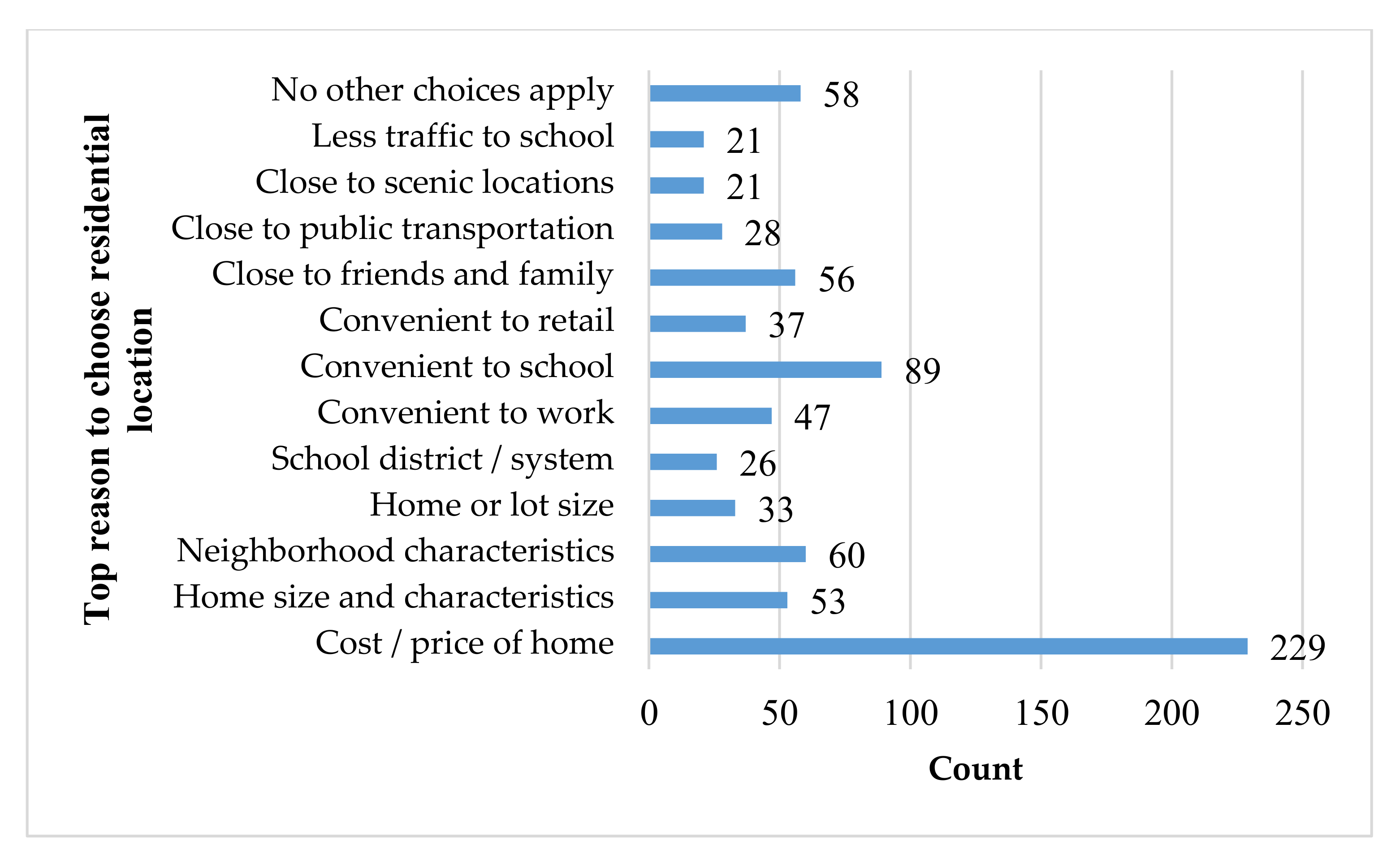
REHOMELOCTop first reason for choosing current home location(1) Cost/price of home; (2) home size and characteristics; (3) neighborhood characteristics; (4) home or lot size; (5) school district/system; (6) convenient for work; (7) convenient for school; (8) convenient for retail (shopping, entertainment, restaurants); (9) close to friends and family; (10) close to public transportation; (11) close to scenic locations (beach, lake, golf courses); (12) less traffic to school; (13) no other choices apply
UTMSUsual travel mode to campus(1) Private car; (2) private motorcycle; (3) public transportation; (4) walking/cycling; (5) metered taxi; (6) ride-sourcing
DISSCDistance from home to campus(1) 0–10 km; (2) 11–20 km; (3) 21–30 km; (4) 31–40 km; (5) 41–50 km; (6) 51–60 km; (7) more than 60 km
ADISSCAcceptable distance from home to campus(1) 0–10 km; (2) 11–20 km; (3) 21–30 km; (4) 31–40 km; (5) 41–50 km; (6) 51–60 km; (7) more than 60 km
Living environment during childhood and adolescence
KSETTLESettlement type during the age periods of 1–6, 7–13, and 14–18(1) city; (2) village; (3) suburb
PCIVILRSPerception towards the size of settlement during the age periods of 7–13 and 14–18(1) very small; (2) small; (3) medium; (4) large; (5) very large
TPHOUSEType of house during the age periods of 7–13 and 14–18(1) bungalow; (2) detached/semi-detached; (3) shop houses; (4) flat (non-gated); (5) apartment (gated); (6) condominium (high rises)
Living environment during childhood and adolescence—density
1DENSITYThe neighborhood I lived in had many shop lots in the age ranges of 7–13 and 14–18(1) strongly disagree; (2) disagree; (3) neutral; (4) agree; (5) strongly agree
2DENSITYThe neighborhood I lived in had many offices in the age ranges of 7–13 and 14–18(1) strongly disagree; (2) disagree; (3) neutral; (4) agree; (5) strongly agree
3DENSITYThe neighborhood I lived in had many residential buildings in the age ranges of 7–13 and 14–18(1) strongly disagree; (2) disagree; (3) neutral; (4) agree; (5) strongly agree
4DENSITYThe neighborhood I lived in had many entertainment facilities in the age ranges of 7–13 and 14–18(1) strongly disagree; (2) disagree; (3) neutral; (4) agree; (5) strongly agree
5DENSITYThe neighborhood I lived in had many industrial facilities in the age ranges of 7–13 and 14–18(1) strongly disagree; (2) disagree; (3) neutral; (4) agree; (5) strongly agree
6DENSITYThe neighborhood I lived in had some schools in the age ranges of 7–13 and 14–18(1) strongly disagree; (2) disagree; (3) neutral; (4) agree; (5) strongly agree
Living environment during childhood and adolescence—diversity
1DIVERSITYMy house was close to the shops in the age ranges of 7–13 and 14–18(1) strongly disagree; (2) disagree; (3) neutral; (4) agree; (5) strongly agree
2DIVERSITYMy house was close to public offices in the age ranges of 7–13 and 14–18(1) strongly disagree; (2) disagree; (3) neutral; (4) agree; (5) strongly agree
3DIVERSITYMy house was close to entertainment facilities in the age ranges of 7–13 and 14–18(1) strongly disagree; (2) disagree; (3) neutral; (4) agree; (5) strongly agree
4DIVERSITYMy house was close to other residential buildings in the age ranges of 7–13 and 14–18(1) strongly disagree; (2) disagree; (3) neutral; (4) agree; (5) strongly agree
5DIVERSITYThe school I attended was within walking distance of my house in the age ranges of 7–13 and 14–18(1) strongly disagree; (2) disagree; (3) neutral; (4) agree; (5) strongly agree
Living environment during childhood and adolescence—design
1DESIGNThe neighborhood I lived in had large block sizes in the age ranges of 7–13 and 14–18(1) strongly disagree; (2) disagree; (3) neutral; (4) agree; (5) strongly agree
2DESIGNThe neighborhood I lived in had many intersections in the age ranges of 7–13 and 14–18(1) strongly disagree; (2) disagree; (3) neutral; (4) agree; (5) strongly agree
3DESIGNThe neighborhood I lived in had a full sidewalk coverage along the street in the age ranges of 7–13 and 14–18(1) strongly disagree; (2) disagree; (3) neutral; (4) agree; (5) strongly agree
4DESIGNThe neighborhood I lived in had many buildings that were set back from the sidewalks with an appropriate distance (there was a good distance between buildings and the sidewalks) in the age ranges of 7–13 and 14–18(1) strongly disagree; (2) disagree; (3) neutral; (4) agree; (5) strongly agree
5DESIGNThe neighborhood I lived in had wide sidewalks in the age ranges of 7–13 and 14–18(1) strongly disagree; (2) disagree; (3) neutral; (4) agree; (5) strongly agree
6DESIGNThe neighborhood I lived in had several pedestrian crossings in the age ranges of 7–13 and 14–18(1) strongly disagree; (2) disagree; (3) neutral; (4) agree; (5) strongly agree
7DESIGNThe neighborhood I lived in had many trees and landscapes in the age ranges of 7–13 and 14–18(1) strongly disagree; (2) disagree; (3) neutral; (4) agree; (5) strongly agree
8DESIGNThe neighborhood I lived in had many pedestrian-related facilities (e.g., water fountains and benches) in the age ranges of 7–13 and 14–18(1) strongly disagree; (2) disagree; (3) neutral; (4) agree; (5) strongly agree
Living environment during childhood and adolescence—destination accessibility
1ACCESSIBILITYIn the neighborhood I lived in, it was easy for me to access local stores in the age ranges of 7–13 and 14–18(1) strongly disagree; (2) disagree; (3) neutral; (4) agree; (5) strongly agree
2ACCESSIBILITYIn the neighborhood I lived in, it was easy for me to access business districts in the age ranges of 7–13 and 14–18(1) strongly disagree; (2) disagree; (3) neutral; (4) agree; (5) strongly agree
3ACCESSIBILITYIn the neighborhood I lived in, it was easy for me to access the primary/secondary school in the age ranges of 7–13 and 14–18(1) strongly disagree; (2) disagree; (3) neutral; (4) agree; (5) strongly agree
4ACCESSIBILITYIn the neighborhood I lived in, it was easy for me to access the recreation facilities in the age ranges of 7–13 and 14–18(1) strongly disagree; (2) disagree; (3) neutral; (4) agree; (5) strongly agree
Living environment during childhood and adolescence—distance to transit
1DISTANCETOTRANIn the neighborhood I lived in, my house was close to the bus stops in the age ranges of 7–13 and 14–18(1) strongly disagree; (2) disagree; (3) neutral; (4) agree; (5) strongly agree
2DISTANCETOTRANIn the neighborhood I lived in, my house was close to the taxi stops in the age ranges of 7–13 and 14–18(1) strongly disagree; (2) disagree; (3) neutral; (4) agree; (5) strongly agree
3DISTANCETOTRANMy school was close to the taxi/bus stops in the age ranges of 7–13 and 14–18(1) strongly disagree; (2) disagree; (3) neutral; (4) agree; (5) strongly agree
Target variable
TTTTOSCTolerable travel time to campus(1) 0–10 min; (2) 11–20 min; (3) 21–30 min; (4) 31–40 min; (5) 41–50 min; (6) 51–60 min; (7) more than 60 min
Table 2. Input variables selected by the Pearson chi-square tests.
RankVariableValueRankVariableValue
1DISSC1.00202DISTANCETOTRAN7130.91
23ACCESSIBILITY7131.0021HHCO0.90
31ACCESSIBILITY7130.99221DIVERSITY7130.89
44DIVERSITY7130.9923PRVE0.87
5RACE0.98245DESIGN14180.87
67DESIGN7130.98254DIVERSITY14180.86
7UTMWS0.98267DESIGN14180.85
83ACCESSIBILITY14180.98274DENSITY7130.85
93DENSITY14180.98282DIVERSITY14180.85
103DENSITY7130.9829KSETTLE160.85
111DIVERSITY14180.97305DESIGN7130.84
12AGE0.96314ACCESSIBILITY7130.81
136DESIGN7130.9432UTMTOSC14180.81
14GEN0.9433UTMTOSC7130.80
152DISTANCETOTRAN14180.93341ACCESSIBILITY14180.80
164ACCESSIBILITY14180.9335REHOMLOC0.79
176DENSITY7130.9336KSETTLE14180.79
18TPHOUSE7130.92372DIVERSITY7130.78
196DENSITY14180.9138EDU0.77
Table 3. Conditional probabilities of high probable TTTs to campus derived from BN#1.
Variable/ValueFrequency (%)
0–1011–2031–4041–5051–60More than 60
TPHOUSE713
110.340.7016.740.040
275.933.35050.060.060
30 0000
43.414.8033.300
510.311.150000
3DENSITY713
110.37.40040.020.0
210.37.4016.740.020.0
337.914.8033.300
431.037.010050.020.00
510.333.300060.0
3DENSITY1418
110.37.4002020
26.911.100600
327.611.1033.300
441.444.410066.7020
513.825.90020.060
4DENSITY713
113.818.5016.700
244.825.9083.340.060.0
331.025.950020.040.0
410.329.650040.00
5000000
6DENSITY713
100016.70
26.93.75016.720.020.0
320.722.250000
462.140.7066.740.040.0
510.333.30040.040.0
6DENSITY1418
1005016.700
26.93.7016.720.020.0
317.218.550000
462.151.905040.040.0
513.825.9016.740.040.0
1DIVERSITY713
103.700040.0
213.814.8033.300
317.214.85033.320.00
455.248.15033.340.040.0
513.818.50040.020.0
1DIVERSITY1418
10100040.0
217.211.1016.700
313.811.1016.720.00
455.263.010050.060.040.0
513.814.8016.720.020.0
Table 4. Conditional probabilities of high probable TTTs to campus derived from BN#2.
Variable/ValueFrequency (%)
0–1011–2031–4041–5051–60More than 60
AGE
178.353.310010050.0100
28.720.00050.00
313.026.70000
4000000
5000000
6000000
EDU
1000000
28.76.733.3000
38.7033.3000
469.666.733.3100.0100.0100.0
5000000
61326.70000
RACE
152.253.366.70075.0
230.426.733.333.3025.0
34.30033.3100.00
413.020.0033.300
UTMS
152.253.366.7100.0100.050.0
226.100000
313.020.033.30050.0
48.726.70000
5000000
6000000
DISSC
187.033.30000
213.046.733.366.750.050.0
3000000
40066.733.350.00
5000000
6000000
7020.000050.0
KSETTLE16
139.166.7100.0050.025.0
239.113.3066.7025.0
321.720.0033.350.050.0
KSETTLE1418
156.560.0100.00100.025.0
234.813.3033.3050.0
38.726.7066.7025.0
TPHOUSE713
18.740.000025.0
278.326.766.733.3100.075.0
3000000
44.313.3066.700
58.720.033.3000
6000000
Publisher’s Note: MDPI stays neutral with regard to jurisdictional claims in published maps and institutional affiliations.

