Hardware-in-the-Loop to Test an MPPT Technique of Solar Photovoltaic System: A Support Vector Machine Approach

Abstract

This paper proposes a new method for maximum power point tracking (MPPT) of the photovoltaic (PV) system while using a DC-DC boost converter. The conventional perturb and observe (P&O) method has a fast tracking response, but it presents oscillation around the maximum power point (MPP) in steady state. Therefore, to satisfy transient and steady-state responses, this paper presents a MPPT method using support vector machines (SVMs). The use of SVM will help to improve the tracking speed of maximum power point of the PV system without oscillations near MPP. A boost converter is used to implement the MPPT method, where the input voltage of the DC-DC converter is regulated using a double loop where the inner loop is a current control that is based on passivity. The MPPT structure is validated by hardware in the loop, a real time and high-speed simulator (PLECS RT Box 1), and a digital signal controller (DSC) are used to model the PV system and implement the control strategies, respectively. The proposed strategy presents low complexity and it is implemented in a commercial low-cost DSC (TI 28069M). The performance of the MPPT proposed is presented under challenging experimental profiles with solar irradiance and temperature variations across the panel. In addition, the performance of the proposed method is compared with the P&O method, which is traditionally most often used in MPPT under demanding tests, in order to demonstrate the superiority of the strategy presented.

1. Introduction

Photovoltaic power generation is a renewable energy source with numerous advantages. Its characteristics in solar energy are recognized by good dynamics that are easy to incorporate into residential microgrids. The low energy conversion efficiency of PV systems is a significant disadvantage in PV systems, notwithstanding, there are important improvements, such as cost reduction, cell efficiency increment, and enhancement in the structural integration of buildings. On the other hand, the surrounding environment, which includes solar irradiance and ambient temperature, affects the amount of energy that is generated by PV systems [1]. Therefore, a control that is associated with maximum power point tracking (MPPT) should provide an appropriate duty cycle, so that DC–DC converters can obtain the maximum level of energy from PV modules [2,3,4]. Several studies for MPPT methods have been developed, with the best-known methods being perturb and observe (P&O) [5], extremum seeking control methods (ESC) [6], and incremental conductance algorithm (INC) [7]. Usually, these methods take the instantaneous values of output voltage of PV module or current to generate the control signals, using a reference voltage, reference current, or duty ratio for maximum power point tracking. The P&O method has the advantages of simple structure and low computational cost. The literature also presents algorithms that are based on estimating the MPP through data with previous values of radiation or temperature. Among them are those based on fuzzy logic (FL) and artificial intelligence (AI) [8]. In order to improve the PV system efficiency, an appropriate DC-DC converter and a MPPT algorithm must be integrated and configured, and the following conditions must be satisfied [9]:

• Fast tracking response (transient response).
• No oscillations around the MPP (steady-state response).
• Response performance against solar irradiance and temperature changes.
• Simple structure with a low computational cost.

Several papers have been published that are related to MPPT algorithms using support vector machines (SVMs). The SVM is a supervised machine learning algorithm that is used for linear regression and problem classification. In [10], the SVM was used as a classifier to generate a large amount of training data that were used to train an artificial neural network. However, this method exhibits power oscillations near the MPP and the used training data set is not satisfactory for generating an accurate learning. In [11], a conventional support vector regression was used to estimate the irradiance levels from PV electrical characteristics, using input features that are not identically and independently distributed (i.i.d), which makes the proposed method complex for implementing on a low-cost microprocessor. In [12], the P&O method has been utilized, where the sized perturbation step was computed using an identification model of solar irradiance based on SVM, for two different locations. However, the selection of the perturb step size is realized off-line for a specific location, updated monthly or seasonally, so that the effects of partial shading is not considered. This paper proposes a novel MPPT algorithm that is based on SVM. The SVM is used to estimate the unknown transfer function of the multivariable non-linear P-V characteristics of a PV module. In machine learning, this problem is known as regression estimation for multiple variables. The main motivations to use the SVM based method are advantages, such as: the ability to estimate the parameters with limited data, robust predictions when nonlinearities and noise appear in the system, and considering all of the inputs and outputs together to construct each regressor [13]. The main contributions of this paper are the following:

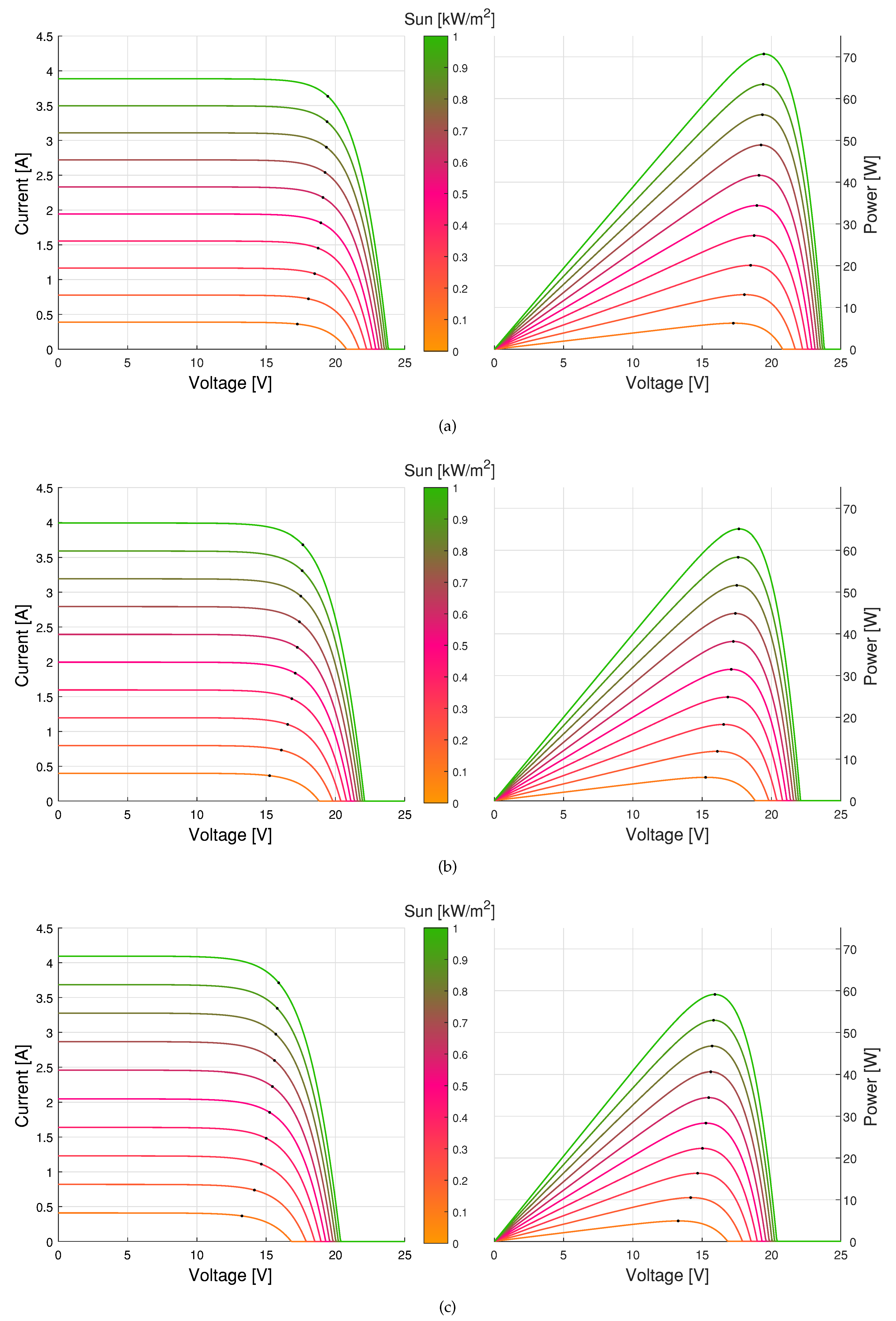
• Provide a new method to determine the MPP of the PV module based on multiple-input multiple-output SVM, without oscillations around the MPP in steady state. The training phase of the SVM only requieres the 10% of the data of the P-V characteristic curves (at different levels of irradiation and temperature) that are given by the manufacturer of the PV module.
• The proposed MPPT algorithm and the double loop control of the DC-DC boost converter can be implemented in a commercial low-cost DSC.
• The performance of the proposed method has been verified through simulations and hardware-in-the loop experiments, showing good accuraccy and reproducibility.

The remaining of this paper is structured, as follows: Section 2 presents the structure of the MPPT control using a DC-DC boost converter. Section 3 describes the proposed MPPT approach. Section 4 presents the simulated and hardware in the loop results. Finally, Section 5 draws the concluding remarks.

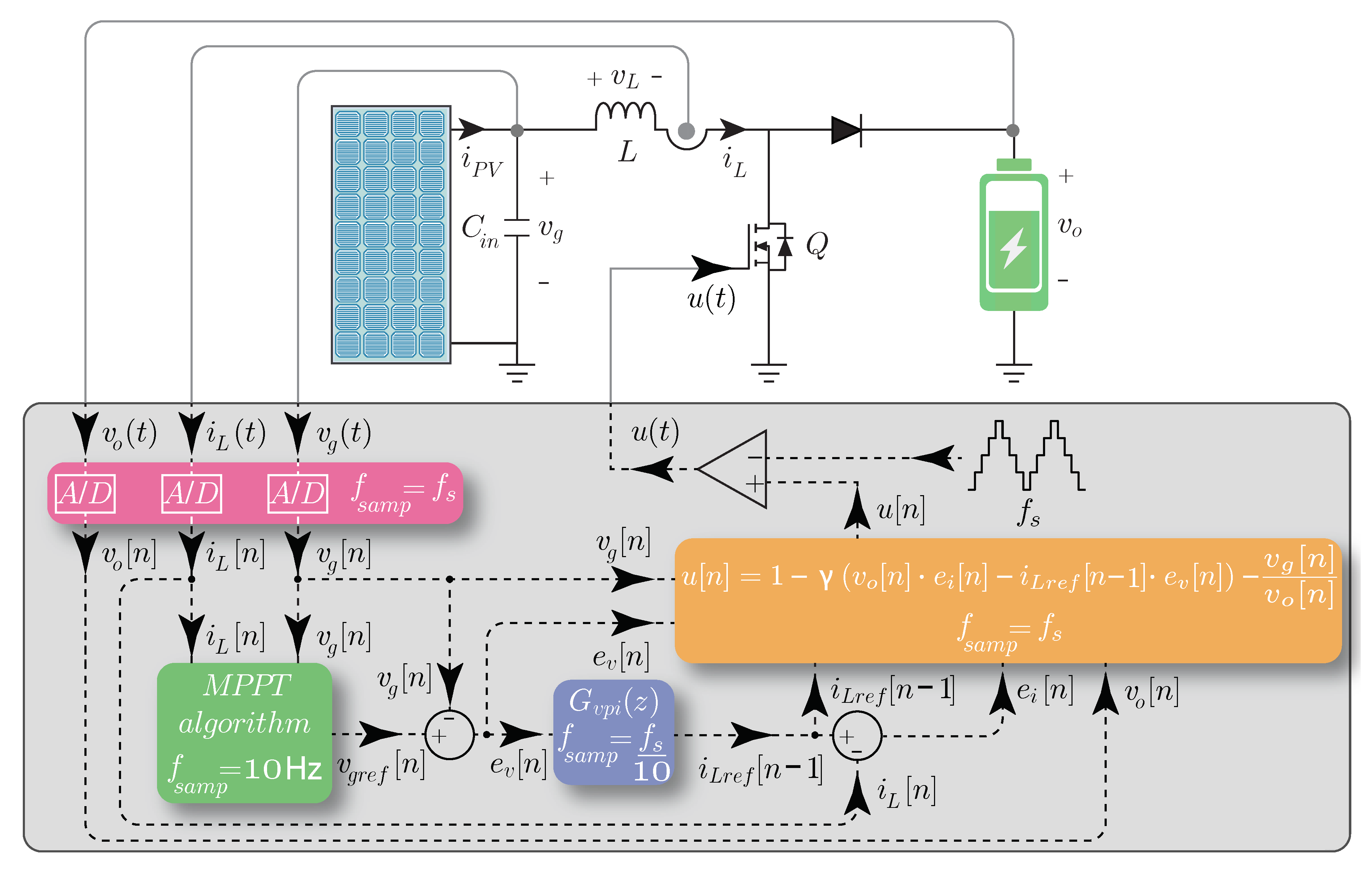
2. MPPT Control by DC-DC Boost Converter

Figure 1 illustrates the MPPT control diagram for a PV module using a DC-DC converter. The PV module supplies voltage and current, converting incident solar radiation into electrical energy through the photoelectric effect, to charge a battery through the DC-DC converter. Figure 2 shows the non-linear I-V characteristic and P-V of the commercial module BP365 for different irradance and ambient temperatures, which include 0 °C, 25 °C, and 50 °C. This PV module is modelled for PLECS simulations, which is presented in [14]. In this work, a boost converter is the selected topology to be used as DC-DC converter. Figure 1 shows the topology of the boost converter. Subsequently, the following system of differential equations for the boost are obtained:

$$\begin{array}{cc}\hfill & {\displaystyle \frac{d{i}_L\left(t\right)}{dt}}={\displaystyle \frac{V_g-(1-u)v_o}{L}}\hfill \end{array}$$

(1)

$$\begin{array}{cc}\hfill & {\displaystyle \frac{d{v}_o\left(t\right)}{dt}}={\displaystyle \frac{-v_o}{R_{L}C}}+{\displaystyle \frac{(1-u)i_L}{C}},\hfill \end{array}$$

(2)

with $i_L$ being the inductor current, $v_o$ the output voltage, and u the control variable $\in \left\{0,1\right\}$. The duty cycle for the boost converter is:

$$\begin{array}{cc}\hfill & \overline{u}=1-{\displaystyle \frac{\overline{v_g}}{\overline{v_o}}}.\hfill \end{array}$$

(3)

2.1. Average Current Control Based on Passivity

The current control that is based on passivity is applied using the output feedback passive in power electronics devices [15]. The system can be written in the following Hamiltonian form:

$$\begin{array}{cc}\hfill & \mathit{D}\dot{e}=\mathit{J}{\displaystyle \frac{\partial H\left(e\right)}{\partial e}}-\mathit{R}{\displaystyle \frac{\partial H\left(e\right)}{\partial e}}+\mathit{c}{e}_u\hfill \\ \\ \hfill & e_y={\mathit{c}}^T{\displaystyle \frac{\partial H\left(e\right)}{\partial e}}.\hfill \end{array}$$

(4)

where $\mathit{D}$ is a positive definite diagonal matrix, $\mathit{J}$ is a skew-symmetric matrix, and $\mathit{R}$ is a symmetric, positive semi-definite, matrix. The matrix $\mathit{J}$ represents the linear terms of the variable control u, $\mathit{R}$ represents the dissipative terms in the system, and the expression $\mathit{c}{e}_u$ is the energy term to control the system. Therefore, the exact regulation error passive output of the system is denoted by $e_y$ [16]. Defining the error as $e=x-\overline{x}$, where $\overline{x}$ is the desired equilibrium of the average states, the state-vector for the systems under study is $x={[i_L,v_o]}^T$, and the error of the input is $e_u=u-\overline{u}$, with the corresponding equilibrium input $\overline{u}$. Being $H=0.5x^{T}x$, doing so, the definition of the error is:

$$\begin{array}{cc}\hfill & x-\overline{x}={\displaystyle \frac{\partial H\left(x\right)}{\partial x}}-{\displaystyle \frac{\partial H\left(\overline{x}\right)}{\partial x}}={\displaystyle \frac{\partial H\left(e\right)}{\partial e}}.\hfill \end{array}$$

(5)

The incremental control input is $e_u=-\gamma e_y$, therefore $u=-\gamma e_y+\overline{u}$, where $\gamma$ is a positive scalar quantity. Consequently, the matrices that represent the dynamics of the exact regulation error for the system (1) and (2) are:

$$\begin{array}{ccc}\hfill & \mathit{D}=\left(\begin{array}{cc}L& 0\\ 0& C\end{array}\right)\hfill & \hfill \mathit{J}=\left(\begin{array}{cc}0& -(1-u)\\ \\ 1-u& -1\\ \end{array}\right)\\ \hfill & \mathit{R}=\left(\begin{array}{cc}0& 0\\ 0& {\displaystyle \frac{1}{R_L}}\end{array}\right)\hfill & \hfill \mathit{c}=\left(\begin{array}{c}{v}_o\\ -i_L\end{array}\right)\end{array}$$

(6)

$$\begin{array}{cc}\hfill & e_y=\overline{v_o}{e}_1-\overline{i_L}{e}_2\hfill \end{array}$$

(7)

The control law for the boost converter is:

$$\begin{array}{cc}\hfill & u=-\gamma (\overline{v_o}{e}_1-\overline{i_L}{e}_2)+1-{\displaystyle \frac{\overline{v_g}}{\overline{v_o}}}\hfill \end{array}$$

(8)

with $e_1=i_L-\overline{i_L}$ and $e_2=v_o-\overline{v_o}$.

2.2. Discrete-Time PI Voltage Control

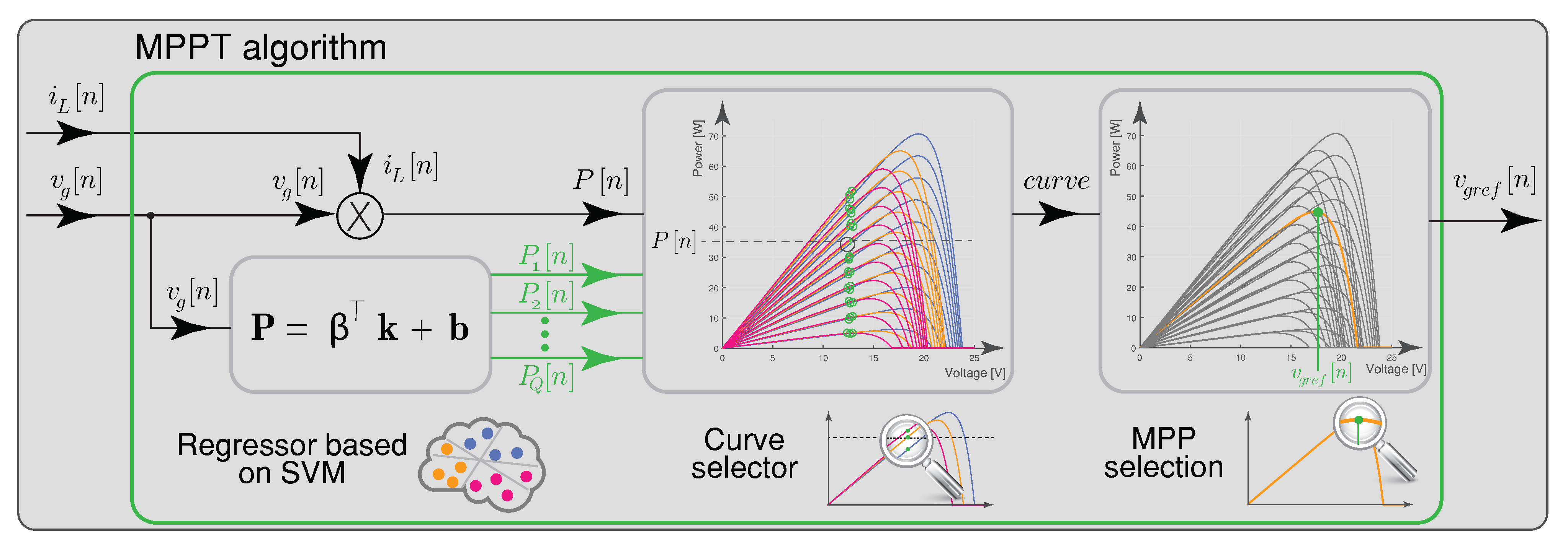
To regulate the input voltage of the boost converter $v_g$, a double loop is implemented while using a proportional-integrator voltage control external loop; this external module gives the input current reference for the inner loop and works with the voltage reference provided by the MPPT algorithm. The controller transfer function can be expressed in the z domain using the forward Euler method, as follows:

$$G_{vpi}\left(z\right)=K_{pv}+\frac{K_{iv}{T}_{samp}}{z-1}.$$

(9)

where $T_{samp}=1/f_{samp}$. The forward-Euler method is used to find the recurrence equation for the discrete-time integral PI control, as follows:

$$\begin{array}{cc}\hfill i_{Lp}\left[n\right]& =K_{pv}{e}_v\left[n\right],\hfill \\ \hfill i_{Li}\left[n\right]& =K_{iv}{T}_{samp}{e}_v\left[n\right]+i_{Li}[n-1],\hfill \\ \hfill i_{Lref}\left[n\right]& =i_{Lp}\left[n\right]+i_{Li}\left[n\right].\hfill \end{array}$$

(10)

where

$$K_{pv}=2\pi {\mathit{f}}_c{C}_{in}$$

(11)

and

$$K_{iv}=\frac{K_{pv}}{T_i},$$

(12)

with $C_{in}$ being the input capacitor, the value of the crossover frequency (CF) for the voltage loop ($f_c$) should be lower than the CF for the current loop. The location of the PI zero should be lower than $f_c$ ($1/\left(2\pi T_i\right)<f_c$).

3. MPPT Algorithm

The Maximum Power Point Tracking (MPPT) control allows a good performance in a PV system under different solar irradiance and temperature values. Usually, the operation of this MPPT is based on the control of the switching converter to extract the maximum power generated by the PV module [17,18]. In this section, the most common and used MPPT method and the proposed MPPT method are presented.

3.1. P&O Method

The P&O MPPT method has been widely used [19,20,21]. It is popular for its simplicity and high tracking capabilities. The aim of this algorithm is tracking the MPP by varying the reference voltage while observing the output power PV module. If the current measured power $P\left[n\right]$ is greater than its previous sampled value $P[n-1]$, then the voltage change is continued in the same direction. Otherwise, it is reversed. The PV module voltage is compared with the maximum voltage in order to predict the MPP. Following this, a small step of reference voltage results in a power step of the PV module [19,22].

3.2. Proposed Support Vector Machine MPPT Method

This subsection presents the proposed MPPT method based on support vector machine. The proposed method requires voltage and current measurements of the PV module, and the dataset of the P-V characteristic curves shown in Figure 2. The maximum power point $(V_m,P_m)$ of each curve are known; therefore, if the operating curve of the PV module is determined, it is possible to know the voltage $V_m$. The operating curve of the PV module is determined as follows: with the actual voltage of the PV module, it is possible to estimate the corresponding powers of all P-V characteristic curves, to this end, the SVM is used to find the mapping between an input voltage and the output powers. The vector $\mathbf{P}={\left[P_1,\dots ,P_Q\right]}^{\top }$ comprises the Q powers of all characteristic curves that correspond to a sample voltage $v_g\left[n\right]$. The relationship between $v_g$ and $\mathbf{P}$ is assumed, as follows [13]:

$$\mathbf{P}={\mathbf{\beta }}^{\top }\mathbf{k}+\mathbf{b},$$

(13)

where matrix $\mathbf{\beta }$ and the vector $\mathbf{b}$ are known as the regressors, which are optimized during the training phase, with an iterative reweighted least squares procedure proposed in [13], and $\mathbf{k}$ is a vector that contains the kernel of the input voltage $v_g\left[n\right]$ and the training voltage measurements. The kernel function that is used in this paper is the radial basis function kernel given as [23]:

$$k(\mathbf{v},v_g\left[n\right])=exp\left(-\frac{\parallel \mathbf{v}-v_g{\left[n\right]\parallel }^2}{2{\sigma }^2}\right),$$

(14)

where the vector $\mathbf{v}$ contains the training samples of voltage, and the hyperparameter $\sigma$ is usually known as the bandwidth. It is worth noting that the datasets taken from the P-V characteristic curves are divided into $10\%$ for training and $90\%$ for validation.

Subsequently, from a given current $i_L\left[n\right]$ and voltage measurements $v_g\left[n\right]$ of the PV module, its actual power $P\left[n\right]$ can be determined. With the vector $\mathbf{P}$ and the actual power $P\left[n\right]$, the actual operating curve (C) of the PV module is determined with the position of the component of $\mathbf{P}$ nearest to $P\left[n\right]$. Once the operating curve is determined, it is possible, with the prior knowledge of the maximum voltage of each curve, to set the voltage $V_m$ for maximum power $P_m$. In brief, the proposed method is described in Figure 3.

4. Results

Different tests have been carried out in order to validate the proposed MPPT algorithm using a DC-DC boost converter. The simulated and hardware in the loop (HIL) results have been presented to show the performance of different controls that integrate the the PV system global control scheme, as shown in Figure 1. The values of the boost converter components are: $L=800 \mathsf{\mu }$H, $C_{in}=88 \mathsf{\mu }$F, switching frequency $f_s=25$ kHz and $V_o=36$ V. Figure 4 shows the HIL setup. The Hardware-in-the-loop (HIL) testing system consists of:

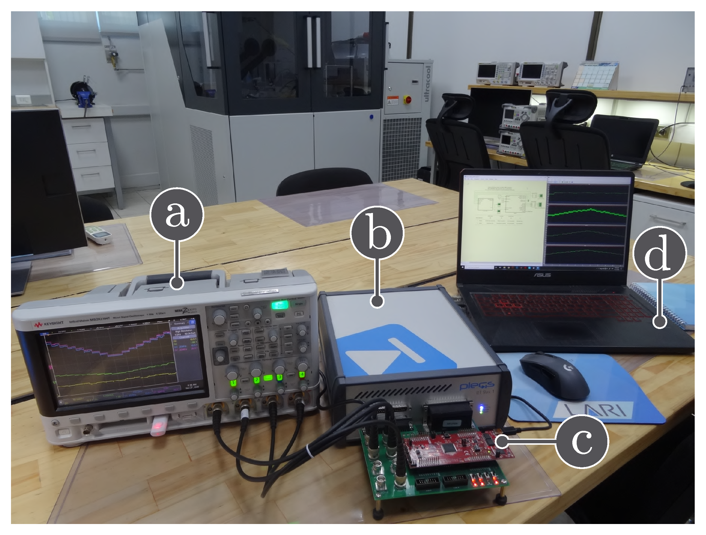
• A TI 28069M LaunchPad.
• An RT Box LaunchPad Interface
• A laptop with the PLECS software.
• An oscilloscope Keysight MSOX2014A.

Where the evaluation kit, a TI 28069M LaunchPad (the red board), is connected to the RT Box via an RT Box LaunchPad Interface (the green board). The plant (PV module and boost converter) has been modelled using PLECS RT Box 1 (Zúrich, Suiza), the sampled time to model the converter is 3 s. In this way, the global control scheme shown in Figure 1 has been implemented using TI28069M LaunchPad of Texas Instruments (TI) (Dallas, TX, USA), which is a low cost TI microcontroller. Inner loop control, double loop control, and MPPT algorithm are validated and the proposed MPPT method is compared with the P&O algorithm. Hence, the realized tests to validate the proposed MPPT algorithm are:

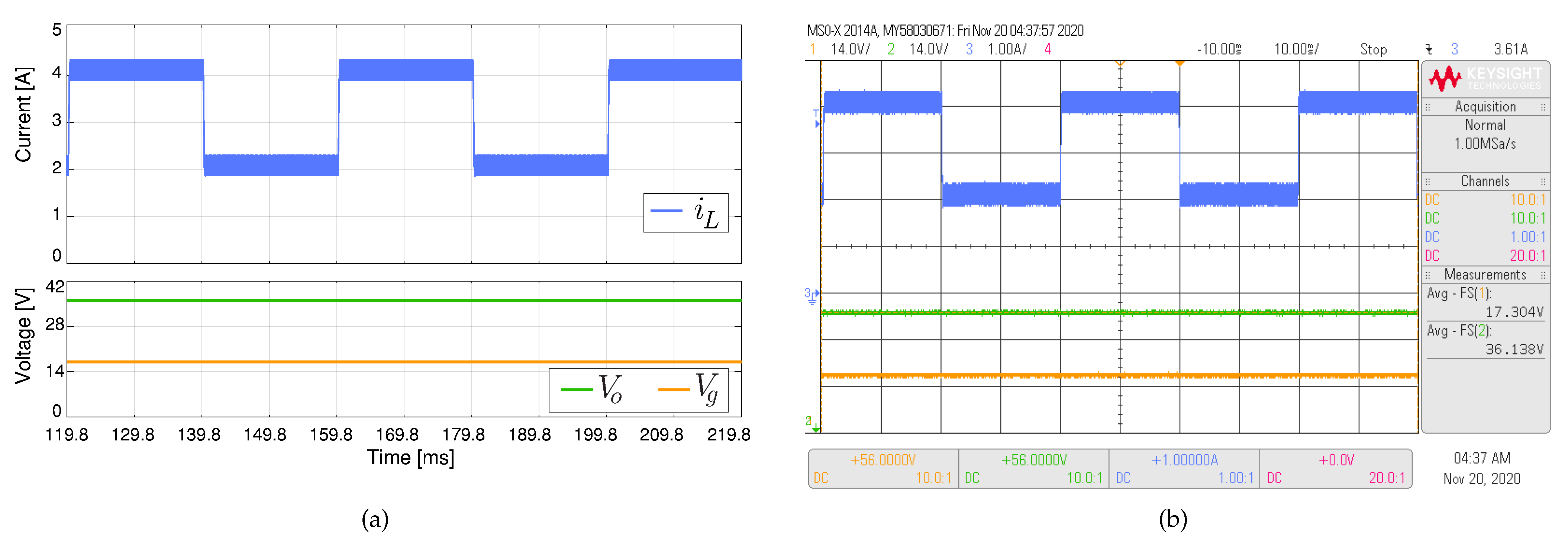
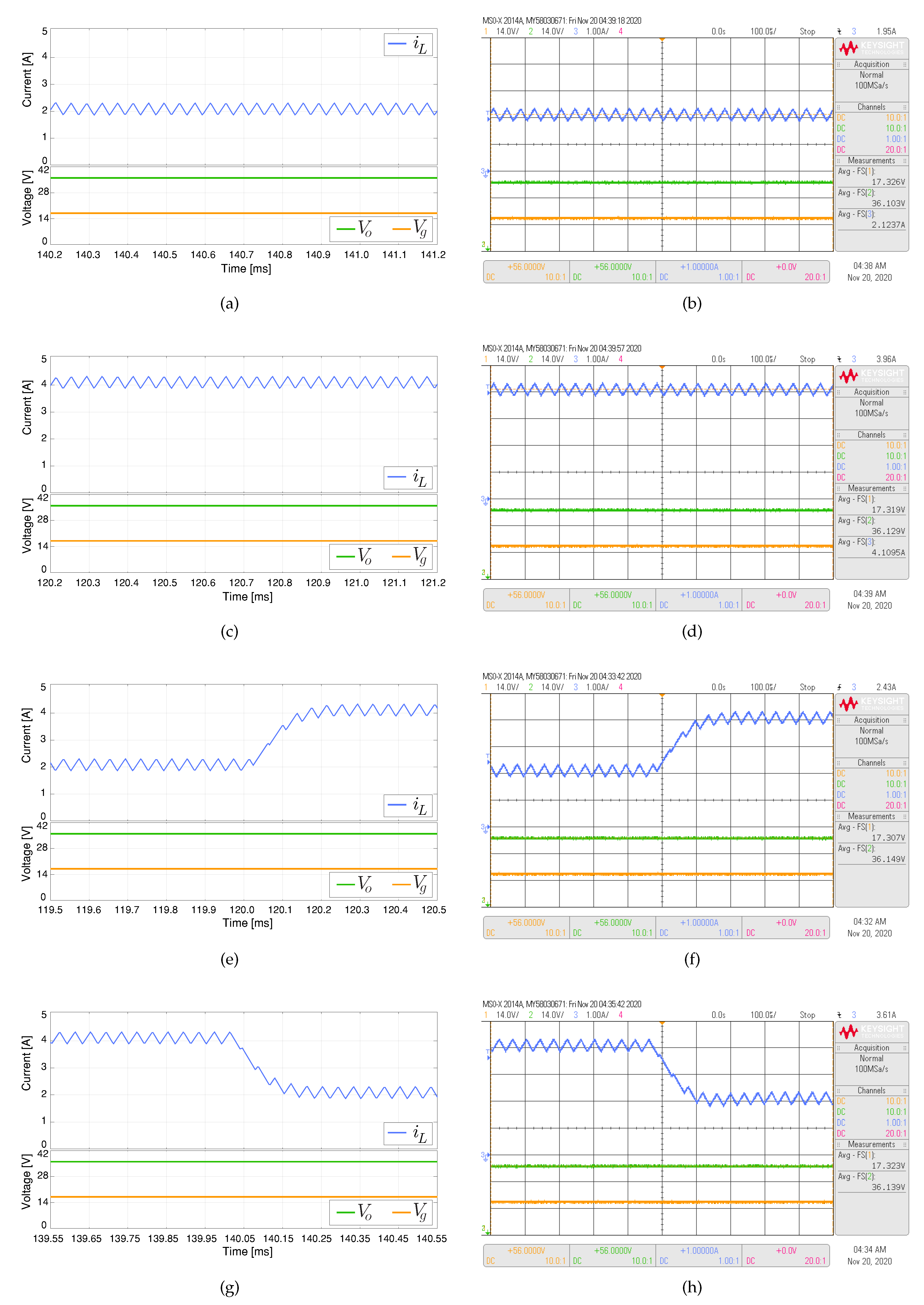
• Inner loop current control test. The current control is validated through a step change of the inductor reference current from 2 A to 6 A and back to 2 A for the current control strategy that is based on passivity.
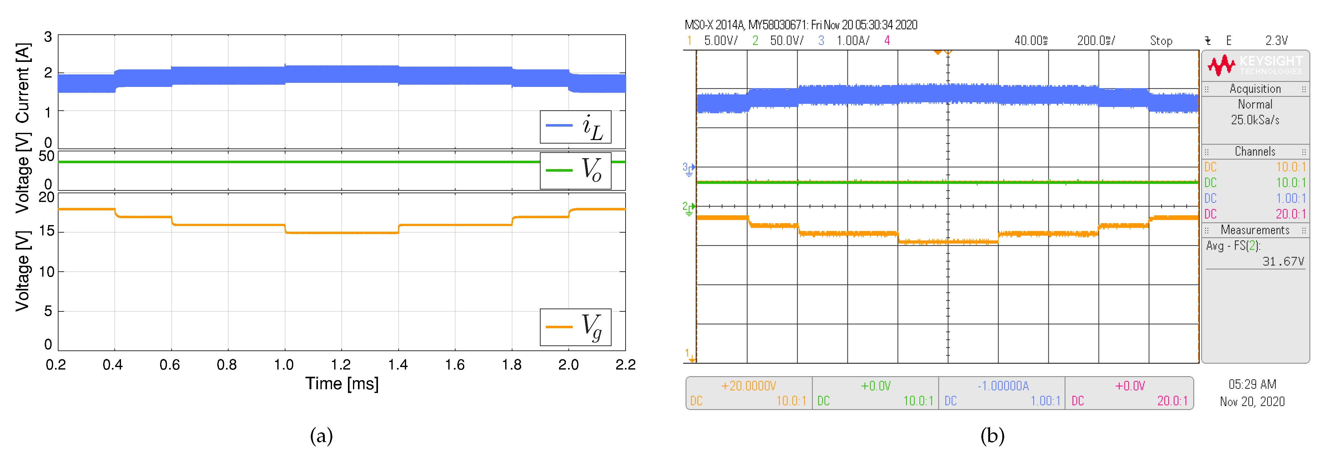
• Double loop control test. Once the inner loop is validated, we proceed to implement a double loop control using an external voltage control to regulate the input voltage (the PV module voltage); this control is a proportional-integrated control; for these tests, voltage reference changes are realized from 15 V to 18 V, in order to demonstrate that the input signal of the converter tracking the reference and the inductor current follow the changes.
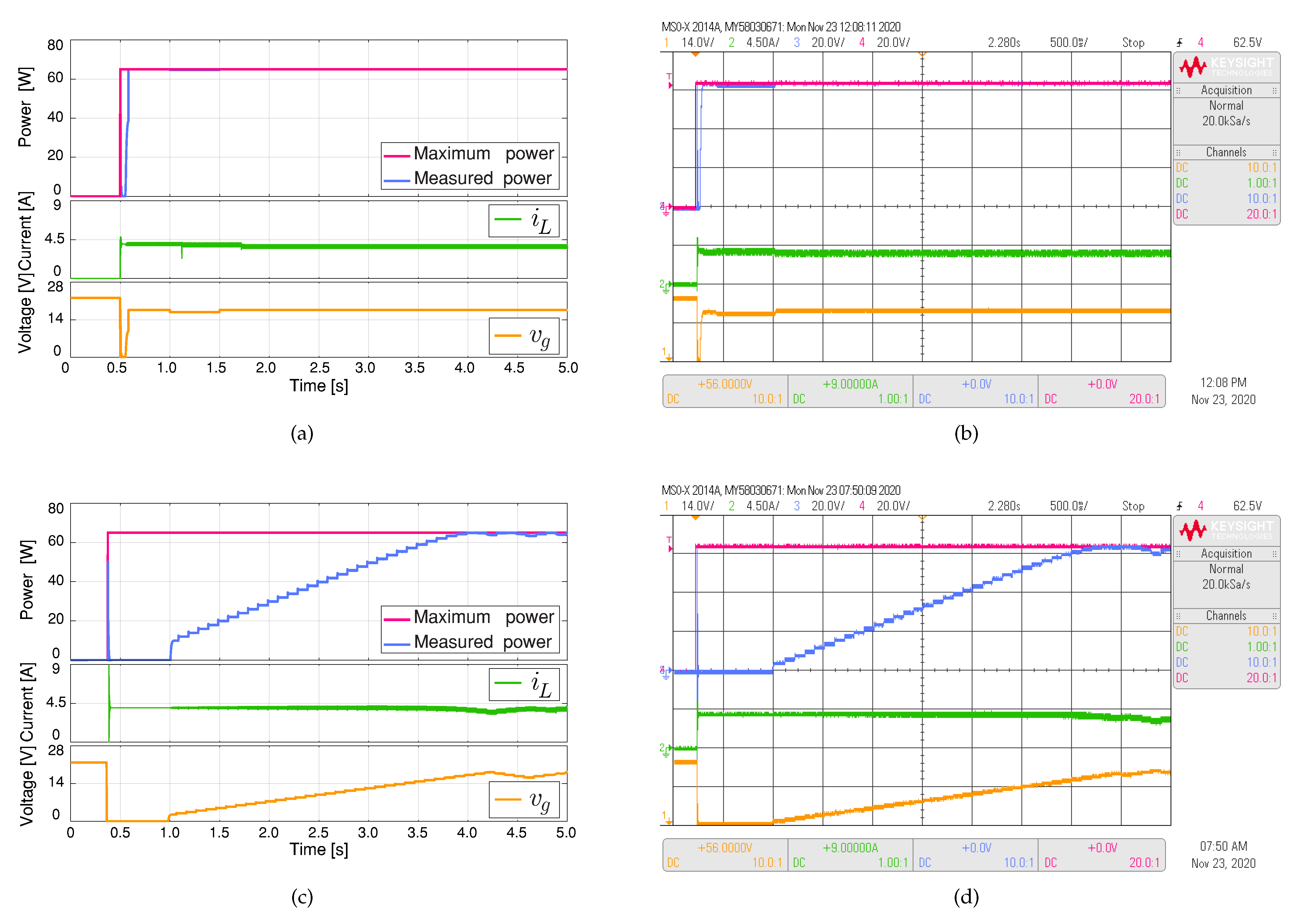
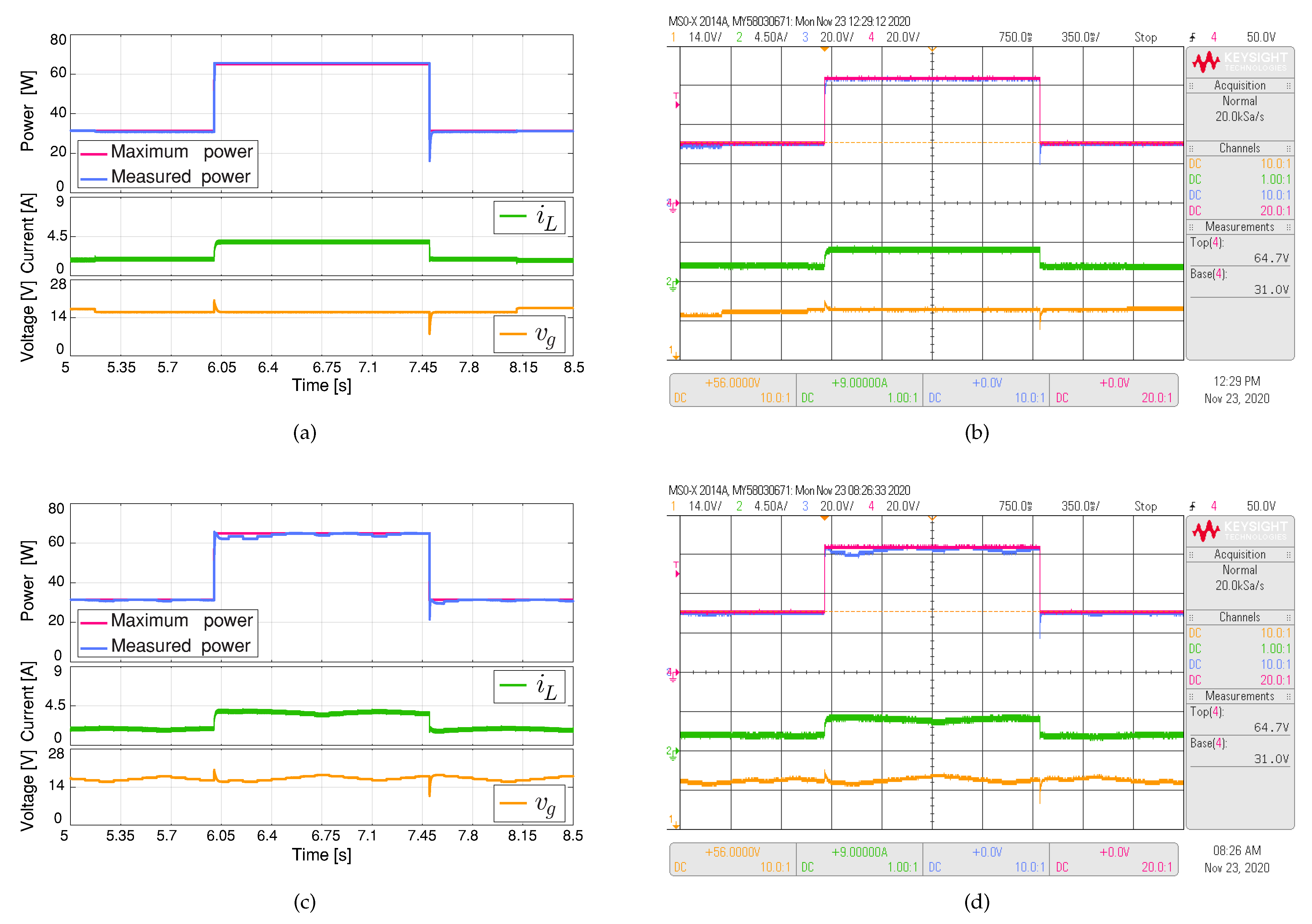
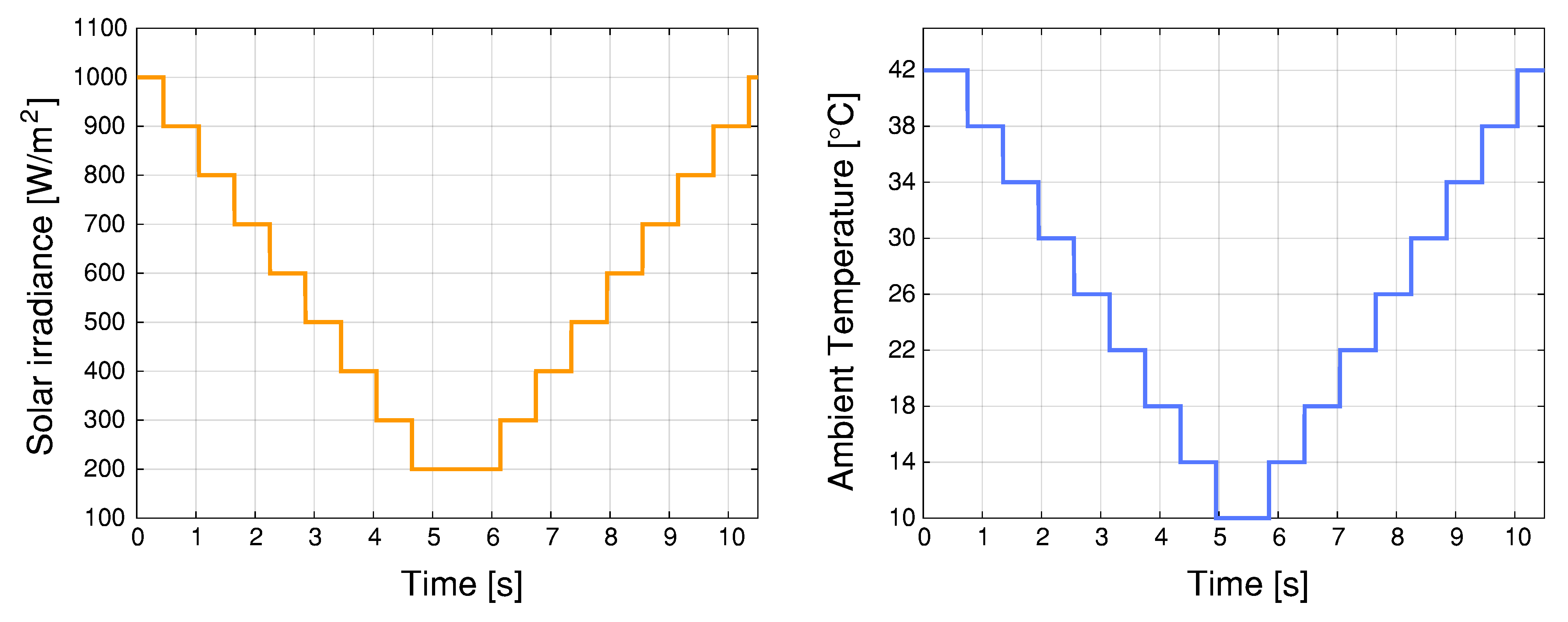
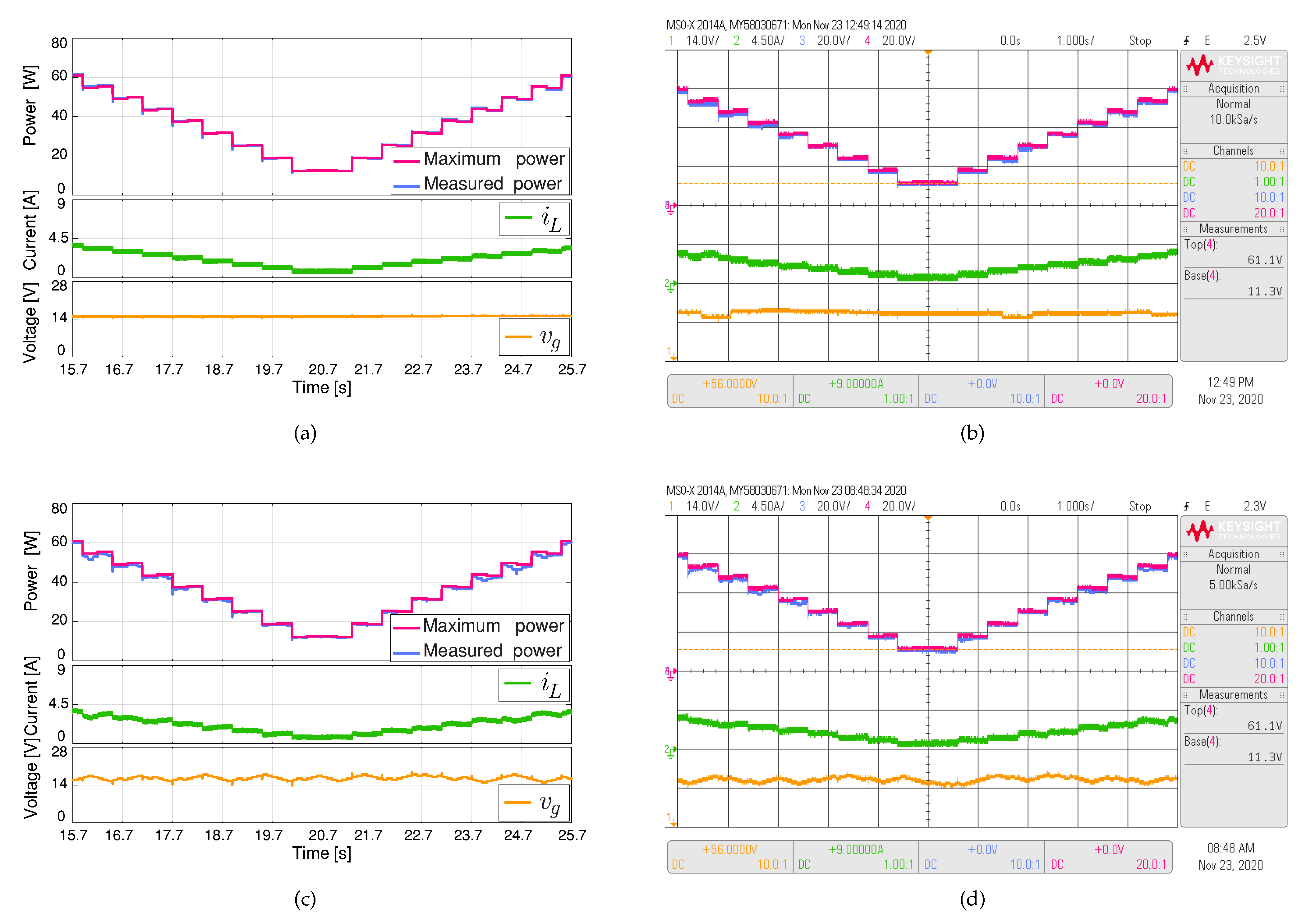
• A comparison with P&O method is realized, where three comparison tests are performed: of the system start-up, of change in irradiance between 1000 W/m${}^2$ and 500 W/m${}^2$, and vice versa, as well as the dynamic behavior of the MPPT algorithms, according to a profile of irrandiance and ambient temperature.

The signals sampled for the control are $v_g$, $v_o$, and $i_L$. The sampling time of the MPPT controller is set to 0.1 s, the sampled time to the voltage regulator is 400 s, which follows the settling time that is required by the DC-DC converter. The switching sampled for the inner current loop is $f_{samp}=f_s=25$ kHz. The PV module used in the simulation is the BP365 65 W, and the electrical characteristic is stated in

Table 1. Electrical characteristics of PV module BP 365.

Electrical Parameters	Value
Maximum power $P_{max}$	65 W
Voltage at maximum power $V_{mp}$	17.6 V
Current at maximum power $I_{mp}$	3.69 A
Short-circuit current $I_{sc}$	3.99 A
Open-circuit voltage $V_{oc}$	22.1 V
Temperature coefficient of short-circuit current	$(0.065\pm 0.015)$%/°C
Temperature coefficient	$-(80\pm 10)$ mV/°C

.

4.1. Inner Loop Current Control Based on Passivity Results

Figure 5 and Figure 6 show the current loop time domain responses for the boost converter. These figures show the simulated and HIL results; the current reference has been changed from 2 A to 6 A and back to 2A. The input voltage is set in 17 V, and the output voltage is $V_o=36$ V. In Figure 5, the transitions during reference changes are smooth, without overshoot and settling times near to 150 s, The simulated results are in good agreement with the experimental results. As shown, the output current is well regulated. The controlled current adequately follows the current reference at all times from the steady–state to the variations in the current reference. Thus, the proposed current control strategy performance during current step reference change is validated. Figure 6 shows the commutations of the current signals, which are in good agreement with the switching frequency of 25 kHz.

4.2. Double Loop Results

Figure 7 shows the simulated and HIL test responses of external loop for voltage references variations from 15 V to 18 V with a step between variations of 1 V. These voltage reference values are in accordance with the maximum power voltage, as can be observed in Figure 2. The selected crossover frequency (CF) corresponds with $f_c=500$ Hz which can allow the calculation of the proportional gain according with (11). The location of the PI zero of Equation (12) is lower than $f_c$ ($1/\left(2\pi T_i\right)<{\mathit{f}}_c$), whereby a $T_i=3.18\times {10}^{-3}$ s was selected. In Figure 1, the voltage regulator ($G_{vpi}\left(z\right)$) calculates the inductor current reference every 400 s.

Figure 7 shows the simulated and HIL responses of voltage loop for a voltage reference variations from 15 V to 18 V with a step between variations of 1 V. This experiment was realized at a fixed ambient temperature of 25${}^{\circ }$ and a fixed irradiance of 600 W/m${}^2$ for the PV module. The voltage reference is accurately tracked and the current transitions caused by the voltage changes are smooth, changing its value with the voltage steps, as can be observed in Figure 7. Hence, the performance of the current control that is based on passivity adding an output voltage loop are validated to be implemented using the MPPT algorithm.

4.3. Comparison of MPPT Methods Results

The MPPT results for the proposed algorithm are compared with the classical P&O algorithm approach. The MPPT algorithms have been implemented to provide a new voltage reference for the voltage loop, every 100 ms, as shown in Figure 1 for the MPPT algorithm block. The exponential function seen in (15) for the proposed MPPT method was efficiently implemented for C code, while using the following approximation:

$$\begin{array}{c}\hfill exp\left(x\right)\approx {\left(1+\frac{x}{n}\right)}^n\end{array}$$

(15)

where n is a positive large integer number, setting $n=256$. Figure 8 presents the simulation and HIL results of the start-up for the MPPT methods. This figure depicts the transient behavior from zero current to an equilibrium point corresponding to the maximum power at a fixed irradiance of 1000 W/m${}^2$ and an ambient temperature of 25 °C for the PV module. In Figure 8a,b, the proposed MPPT reaches the steady state near to 2 s, while, for the P&O method in Figure 8c,d, the steady state is reached in around 6 s, with the proposed MPPT having a faster tracking than the P&O method during system start-up. It is important to note that the P&O algorithm generates an oscillating signal around the maximum. The proposed MPPT algorithm works at the optimum point, and there is no oscillation after it has been tracked.

Figure 9 shows the simulated and HIL results of the MPP tracking performance under step irradiation variations from 500 W to 1000 W and returning to 500 W with a fixed ambient temperature of 25 °C. Figure 9a,b present the results for the proposed MPPT and Figure 9c,d show the results for the P&O algorithm. The MPPT efficiency values were calculated using the following equation:

$$\begin{array}{c}\hfill {\eta }_{MPPT}={\displaystyle \frac{1}{T_m}}\sum \frac{v_g{i}_{PV}}{P_{mpp}}\Delta T\end{array}$$

(16)

where $P_{mpp}$ is the available MPP power of the solar module, $\Delta T$ is the sampling time (0.1 s), and $T_m$ is the overall time interval measurement. The overall MPPT tracking efficiency for the test presented in Figure 9 is 97.56% for the P&O method and 99.46% for the proposed MPPT. For the classical P&O method, the PV system always operates in an oscillating mode, as can be observed by the inductor current and input voltage of the converter in Figure 9c,d. Therefore, the proposed MPPT method achieves a superior performance during abrupt irradiation variations than the classical P&O method.

The system is tested and the MPPT methods are compared over the irradiance and ambient temperature profile that is shown in Figure 10. This test probes the controller’s robustness and the ability to keep extracting the maximum power within these abrupt variations. Figure 11a,b, for the proposed MPPT, present an overall MPPT tracking efficiency of 99.3%, while, for the P&O method, the tracking efficiency is 97% in Figure 11c,d. Moreover, the proposed MPPT does not present oscillations signals (power, current, and input voltage) when compared with the P&O.

Table 2. Comparative analysis of the MPPT methods during the star-up.

Criteria	P&O	MPPT-Proposed Algorithm
Settling time [s]	2.98	0.08
Power ripple [W]	1.81	0.26
Mean power tracked [W]	44.93	58.46
Power at global maximum [W]	64.98	64.98
Tracking factor [%]	70.08	95.53

shows the quantitative analysis of the proposed MPPT method and P&O method for the results that are shown in Figure 8. This table demonstrates a high performance of the proposed MPPT method during the start-up in comparison to the P&O method; when presenting a high tracking factor, the mean power tracked value is close to the power global maximum and the setting time is short.

Table 3. Comparative analysis of the MPPT methods under irradiation variations.

Criteria	P&O	MPPT-Proposed Algorithm
RE	5.598	2.710
MAE	0.521	0.476
RMSE	0.919	0.714

shows the sensitivity of the algorithms by mean absolute error (MAE), relative error (RE), and root means square error (RMSE) for the results that are shown in Figure 9. The standard error equations are given in [24]:

$$\begin{array}{c}\hfill RE=\frac{{\sum }_{i=1}^m(P_{pvi}-P_{mpp})}{P_{mpp}}100\%\end{array}$$

(17)

$$\begin{array}{c}\hfill MAE=\frac{{\sum }_{i=1}^m|P_{pvi}-P_{mpp}|}{m}\end{array}$$

(18)

$$\begin{array}{c}\hfill RMSE=\sqrt{\frac{{\sum }_{i=1}^m{(P_{pvi}-P_{mpp})}^2}{m}}\end{array}$$

(19)

where $P_{pvi}$ represents the power of the PV module and m represents the number of samples. The standard errors values indicated that the performance of the proposed MPPT algorithm has a higher effectiveness to tracking the maximum power point.

Table 4. General comparison of the studied MPPT methods.

MPPT Algorithm	P&O	MPPT-Proposed Algorithm
Parameters knowledge	Not necessary	Not necessary
Complexity	Low	Moderate
Oscillation around MPP	Yes	No
Parameter tuning	No	No
Convergence speed	Slow	Fast
Overall efficiency	Medium	High
Precision	Low	High

shows a summary of MPPT techniques comparison, where the proposed MPPT is highlighted for its high efficiency and precision.

5. Conclusions

This paper proposes a method for tracking the MPP of a PV system. P&O is commonly used as a MPPT strategy of PV systems, but it uses a constant voltage step to obtain the tracking power limits its performance. In this paper, a MPPT control that is based on SVM is proposed to avoid oscillations around the MPP. The proposed MPPT method works, as follows: an SVM is used to estimate the non-linear P-V characteristic of a PV module through regression estimation for multiple variables with scarse training data, and this information is then used to select the optimal output reference voltage. Hardware in the loop tests show that the proposed MPPT has a better performance and efficiency in comparison to the P&O method for constant and varying weather conditions. The model of the power system was modelled by PLECS simulation tool using a RT Box 1 and the control strategies were implemented in a commercial low-cost DSC using C programming software. In this way, it is demonstrated that the proposed strategy has the advantage of a moderate computational cost that allows it to be implemented in low-cost DSC. Future research will address the study of shading in solar panels extending the proposed SVM-based method.

References

1. Khan, R.; Khan, L.; Ullah, S.; Sami, I.; Ro, J.S. Backstepping Based Super-Twisting Sliding Mode MPPT Control with Differential Flatness Oriented Observer Design for Photovoltaic System. Electronics 2020, 9, 1543. [Google Scholar] [CrossRef]
2. Seyedmahmoudian, M.; Kok Soon, T.; Jamei, E.; Thirunavukkarasu, G.S.; Horan, B.; Mekhilef, S.; Stojcevski, A. Maximum power point tracking for photovoltaic systems under partial shading conditions using bat algorithm. Sustainability 2018, 10, 1347. [Google Scholar] [CrossRef] [Green Version]
3. Al-Majidi, S.D.; Abbod, M.F.; Al-Raweshidy, H.S. Design of an Efficient Maximum Power Point Tracker Based on ANFIS Using an Experimental Photovoltaic System Data. Electronics 2019, 8, 858. [Google Scholar] [CrossRef] [Green Version]
4. González-Castaño, C.; Lorente-Leyva, L.L.; Muñoz, J.; Restrepo, C.; Peluffo-Ordóñez, D.H. An MPPT Strategy Based on a Surface-Based Polynomial Fitting for Solar Photovoltaic Systems Using Real-Time Hardware. Electronics 2021, 10, 206. [Google Scholar] [CrossRef]
5. Mohammad, A.N.M.; Radzi, M.A.M.; Azis, N.; Shafie, S.; Zainuri, M.A.A.M. An Enhanced Adaptive Perturb and Observe Technique for Efficient Maximum Power Point Tracking Under Partial Shading Conditions. Appl. Sci. 2020, 10, 3912. [Google Scholar] [CrossRef]
6. Hammami, M.; Ricco, M.; Ruderman, A.; Grandi, G. Three-phase three-level flying capacitor PV generation system with an embedded ripple correlation control MPPT algorithm. Electronics 2019, 8, 118. [Google Scholar] [CrossRef] [Green Version]
7. Moussa, I.; Khedher, A.; Bouallegue, A. Design of a low-cost PV emulator applied for PVECS. Electronics 2019, 8, 232. [Google Scholar] [CrossRef] [Green Version]
8. Wang, Y.; Yang, Y.; Fang, G.; Zhang, B.; Wen, H.; Tang, H.; Fu, L.; Chen, X. An advanced maximum power point tracking method for photovoltaic systems by using variable universe fuzzy logic control considering temperature variability. Electronics 2018, 7, 355. [Google Scholar] [CrossRef] [Green Version]
9. Kim, J.C.; Huh, J.H.; Ko, J.S. Improvement of MPPT control performance using fuzzy control and VGPI in the PV system for micro grid. Sustainability 2019, 11, 5891. [Google Scholar] [CrossRef] [Green Version]
10. Farayola, A.; Hasan, A.; Ali, A. Efficient photovoltaic mppt system using coarse gaussian support vector machine and artificial neural network techniques. Int. J. Innov. Comput. Inf. Control. 2018, 14, 323–339. [Google Scholar] [CrossRef]
11. Ma, J.; Jiang, H.; Huang, K.; Bi, Z.; Man, K.L. Novel Field-Support Vector Regression-Based Soft Sensor for Accurate Estimation of Solar Irradiance. IEEE Trans. Circuits Syst. Regul. Pap. 2017, 64, 3183–3191. [Google Scholar] [CrossRef]
12. Yan, K.; Du, Y.; Ren, Z. MPPT Perturbation Optimization of Photovoltaic Power Systems Based on Solar Irradiance Data Classification. IEEE Trans. Sustain. Energy 2019, 10, 514–521. [Google Scholar] [CrossRef]
13. Sánchez-Fernández, M.; de Prado-Cumplido, M.; Arenas-García, J.; Pérez-Cruz, F. SVM multiregression for nonlinear channel estimation in multiple-input multiple-output systems. IEEE Trans. Signal Process. 2004, 52, 2298–2307. [Google Scholar] [CrossRef]
14. Schönberger, J. Modeling a Photovoltaic String using PLECS. In Application Example, Ver; Internal Report Plexim: Zürich, Switzerland, 2013; pp. 4–13. [Google Scholar]
15. Sira-Ramirez, H.J.; Silva-Ortigoza, R. Control Design Techniques in Power Electronics Devices; Springer Science & Business Media: Berlin/Heidelberg, Germany, 2006. [Google Scholar]
16. García-Rodríguez, V.H.; García-Sánchez, J.R.; Silva-Ortigoza, R.; Hernández-Márquez, E.; Taud, H.; Ponce-Silva, M.; Saldaña-Gonzalez, G. Passivity Based Control for the “Boost Converter-Inverter-DC Motor” System. In Proceedings of the 2017 International Conference on Mechatronics, Electronics and Automotive Engineering (ICMEAE), Morelos, México, 21–24 November 2017; pp. 77–81. [Google Scholar]
17. Farhat, M.; Barambones, O.; Sbita, L. A new maximum power point method based on a sliding mode approach for solar energy harvesting. Appl. Energy 2017, 185, 1185–1198. [Google Scholar] [CrossRef]
18. Pagola, V.; Peña, R.; Segundo, J.; Ospino, A. Rapid Prototyping of a Hybrid PV–Wind Generation System Implemented in a Real-Time Digital Simulation Platform and Arduino. Electronics 2019, 8, 102. [Google Scholar] [CrossRef] [Green Version]
19. Kamran, M.; Mudassar, M.; Fazal, M.R.; Asghar, M.U.; Bilal, M.; Asghar, R. Implementation of improved Perturb & Observe MPPT technique with confined search space for standalone photovoltaic system. J. King Saud Univ. Eng. Sci. 2018. [Google Scholar] [CrossRef]
20. Kollimalla, S.K.; Mishra, M.K. A novel adaptive P&O MPPT algorithm considering sudden changes in the irradiance. IEEE Trans. Energy Convers. 2014, 29, 602–610. [Google Scholar]
21. Ahmed, J.; Salam, Z. A modified P&O maximum power point tracking method with reduced steady-state oscillation and improved tracking efficiency. IEEE Trans. Sustain. Energy 2016, 7, 1506–1515. [Google Scholar]
22. Andrean, V.; Chang, P.C.; Lian, K.L. A review and new problems discovery of four simple decentralized maximum power point tracking algorithms—Perturb and observe, incremental conductance, golden section search, and Newton’s quadratic interpolation. Energies 2018, 11, 2966. [Google Scholar] [CrossRef] [Green Version]
23. Schölkopf, B.; Smola, A. Learning with Kernels; MIT Press: Cambridge, MA, USA, 2001. [Google Scholar]
24. Zafar, M.H.; Al-shahrani, T.; Khan, N.M.; Feroz Mirza, A.; Mansoor, M.; Qadir, M.U.; Khan, M.I.; Naqvi, R.A. Group Teaching Optimization Algorithm Based MPPT Control of PV Systems under Partial Shading and Complex Partial Shading. Electronics 2020, 9, 1962. [Google Scholar] [CrossRef]
Figure 1. Block diagram of the digital controller for the Maximum Power Point Tracking (MPPT) of the boost converter.
Sustainability 13 03000 g001
Figure 2. Curve PV module I-V characteristic (a) 0 °C temperature, (b) 25 °C and (c) 50 °C.
Sustainability 13 03000 g002
Figure 3. Block diagram of the proposed MPPT method based on support vector machine.
Sustainability 13 03000 g003
Figure 4. Hardware in-the-loop experimental setup: (a) oscilloscope, (b) PLECS RT-box, (c) Texas Instruments LAUNCHXL-F28069M, and (d) Laptop.
Sustainability 13 03000 g004
Figure 5. Simulated (a) and experimental (b) responses of the current control based on passivity when the reference i r e f changes with steps of 2 A with an input voltage V g = 17 V and an output voltage V o = 36 V. CH1: v g (14 V/div), CH2: V o (14 V/div), CH3: i L (1A/div), and a time base of 10 ms.
Sustainability 13 03000 g005
Figure 6. Simulated (a,c,e,g) and experimental (b,d,f,h) responses of the input current control based on passivity when the reference i r e f : (a,b) is equal to 2 A, (c,d) is equal to 4 A, (e,f) changes from 2 A to 4 A, and (g,h) from 4 A to 2 A. The converter is operating with an input voltage V g = 17 V and an output voltage V o = 36 V). CH1: V g (14 V/div), CH2: V o (14 V/div), CH3: i L (1A/div) and a time base of 100 s.
Sustainability 13 03000 g006
Figure 7. Simulated (a) and experimental (b) responses of the current control based on passivity when the reference v r e f changes with steps of 1 V between 15 V to 18 V while the output voltage ( V o = 36 V) ensures a boost operation. CH1: v g (5 V/div), CH2: V o (50 V/div), CH3: i L (1A/div), and a time base of 200 ms.
Sustainability 13 03000 g007
Figure 8. Simulated (a,c) and experimental (b,d) dynamic behavior of the MPPT algorithms during system start-up with an irradiance of 1000 W/m 2 and an output voltage V o = 36 V. The proposed MPPT algorithm (top) is compared with the perturb and observe (P&O) based MPPT algorithm (bottom). CH1: v g (14 V/div), CH2: i L (4.5 A/div), CH3: Maximum power (20 W/div), CH4: Measured power (20 W/div) and a time base of 500 ms.
Sustainability 13 03000 g008
Figure 9. Simulated (a,c) and experimental (b,d) dynamic behavior of the MPPT algorithms dealing with sudden changes in irradiance between 1000 W/m 2 and 500 W/m 2 and vice versa. Output voltage V o = 36 V. The proposed MPPT algorithm (top) is compared with the perturb and observe (P&O) based MPPT algorithm (bottom). CH1: v g (14 V/div), CH2: i L (4.5 A/div), CH3: Maximum power (20 W/div), CH4: Measured power (20 W/div), and a time base of 350 ms.
Sustainability 13 03000 g009
Figure 10. Irradiance and ambient temperature profile.
Sustainability 13 03000 g010
Figure 11. Simulated (a,c) and experimental (b,d) dynamic behavior of the MPPT algorithms dealing with changes in irradiance and temperature according to the profile shown in Figure 10. Output voltage V o = 36 V. The proposed MPPT algorithm (top) is compared with perturb and observe (P&O) based MPPT algorithm (bottom). CH1: v g (14 V/div), CH2: i L (4.5 A/div), CH3: Maximum power (20 W/div), CH4: Measured power (20 W/div) and a time base of 1 s.
Sustainability 13 03000 g011