
Contextual Route Recommendation System in Heterogeneous Traffic Flow

 ,
,
Abstract
:1. Introduction
2. Literature Review
2.1. Prediction of Traffic Condition
2.2. Route Recommendation
Attributes of Road Situation
3. Proposed Systems
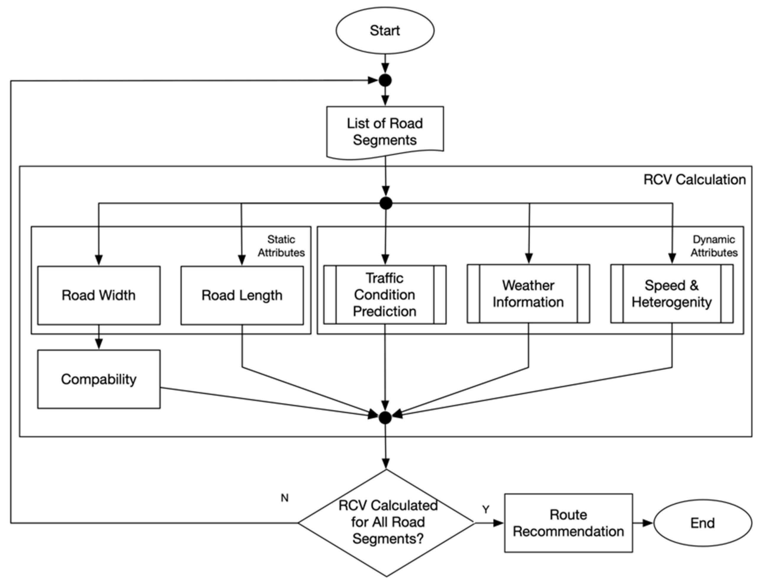
3.1. RCV Calculation
3.1.1. Compatibility
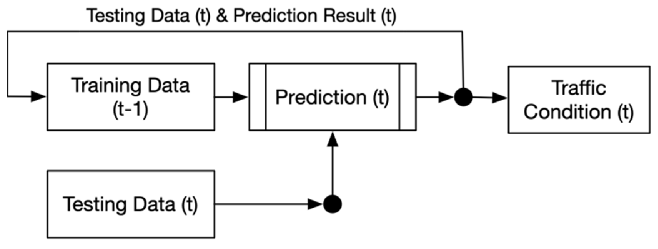
3.1.2. Prediction of Traffic Condition
3.1.3. Weather, Average Vehicle’s Speed, and Heterogeneity
3.2. Route Recommendation
4. Results and Discussions
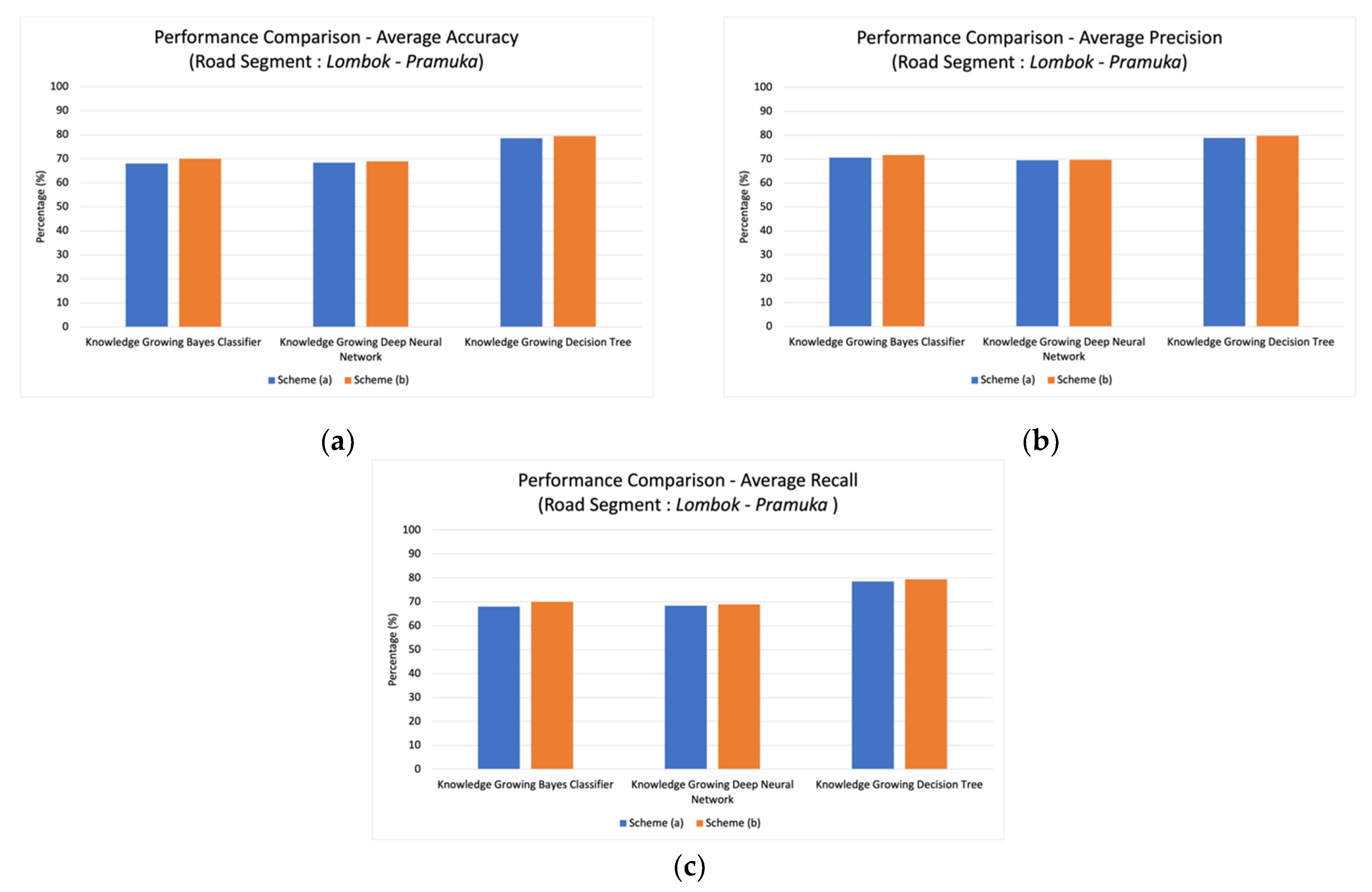
4.1. Prediction System of Traffic Condition
4.2. The Calculation of RCV
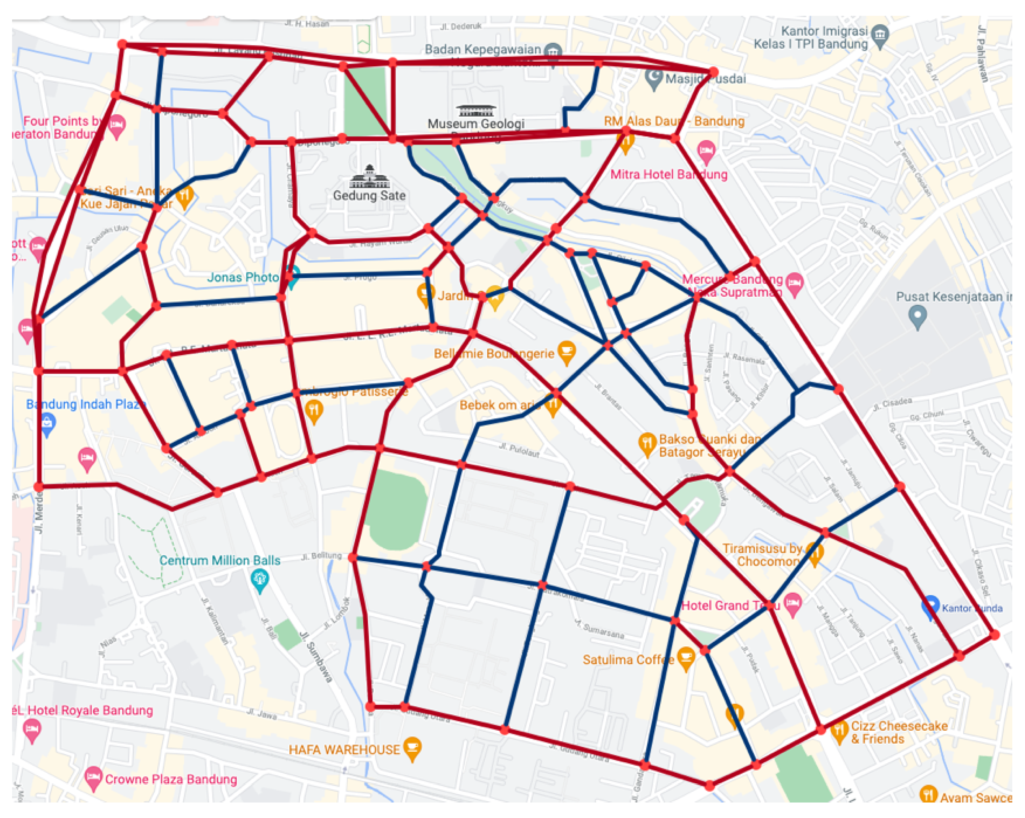
4.3. Route Recommendation
4.3.1. Simulation of Recommended Route Based on Variances of Travel Distance
4.3.2. Comparison of Recommended Route Based on Variances of Attributes
5. Conclusions
Author Contributions
Funding
Institutional Review Board Statement
Informed Consent Statement
Data Availability Statement
Conflicts of Interest
References
- Liu, L.; Xu, J.; Liao, S.S.; Chen, H. A Real-Time Personalized Route Recommendation System for Self-Drive Tourists Based on Vehicle to Vehicle Communication. Expert Syst. Appl. 2014, 41, 3409–3417. [Google Scholar] [CrossRef]
- Shaout, A.; Colella, D.; Awad, S. Advanced Driver Assistance Systems—Past, Present and Future. In Proceedings of the 2011 Seventh International Computer Engineering Conference (ICENCO’2011), Cairo, Egypt, 27–28 December 2011; pp. 72–82. [Google Scholar] [CrossRef]
- BPS—Statictics Indonesia. Perkembangan Jumlah Kendaraan Bermotor Menurut Jenis, 1949–2016; BPS—Statictics Indonesia: Jakarta, Indonesia, 2018.
- Naumann, M.; Lauer, M.; Stiller, C. Generating Comfortable, Safe and Comprehensible Trajectories for Automated Vehicles in Mixed Traffic. In Proceedings of the 2018 21st International Conference on Intelligent Transportation Systems (ITSC), Maui, HI, USA, 4–7 November 2018; pp. 575–582. [Google Scholar] [CrossRef] [Green Version]
- Wedagama, D.M.P. The Influence of Mixed Traffic on Congestion Level. Int. J. GEOMATE 2019, 17, 18–25. [Google Scholar] [CrossRef]
- Afrin, T.; Yodo, N. A Survey of Road Traffic Congestion Measures towards a Sustainable and Resilient Transportation System. Sustainability 2020, 12, 4660. [Google Scholar] [CrossRef]
- European Conference of Ministers of Transportation. Managing Urban Traffic Congestion; OECD Publishing: Paris, France, 2007; Volume 9789282101. [Google Scholar] [CrossRef] [Green Version]
- Zadobrischi, E.; Cosovanu, L.M.; Dimian, M. Traffic Flow Density Model and Dynamic Traffic Congestion Model Simulation Based on Practice Case with Vehicle Network and System Traffic Intelligent Communication. Symmetry 2020, 12, 1172. [Google Scholar] [CrossRef]
- Alirezaei, M.; Onat, N.; Tatari, O.; Abdel-Aty, M. The Climate Change-Road Safety-Economy Nexus: A System Dynamics Approach to Understanding Complex Interdependencies. Systems 2017, 5, 6. [Google Scholar] [CrossRef]
- Akin, D.; Sisiopiku, V.P.; Skabardonis, A. Impacts of Weather on Traffic Flow Characteristics of Urban Freeways in Istanbul. Procedia—Soc. Behav. Sci. 2011, 16, 89–99. [Google Scholar] [CrossRef] [Green Version]
- Rahman, F.I.; Hasnat, A.; Lisa, A.A. Traffic Flow Prediction by Incorporating Weather Information in Naïve Bayes Classifier. J. Adv. Civ. Eng. Pract. Res. 2019, 8, 10–16. [Google Scholar]
- Omranian, E.; Sharif, H.; Dessouky, S.; Weissmann, J. Exploring Rainfall Impacts on the Crash Risk on Texas Roadways: A Crash-Based Matched-Pairs Analysis Approach. Accid. Anal. Prev. 2018, 117, 10–20. [Google Scholar] [CrossRef] [PubMed]
- Ali, Q.; Yaseen, M.R.; Khan, M.T.I. The Impact of Temperature, Rainfall, and Health Worker Density Index on Road Traffic Fatalities in Pakistan. Environ. Sci. Pollut. Res. 2020, 27, 19510–19529. [Google Scholar] [CrossRef] [PubMed]
- Afshari, A.; Schuch, F.; Marpu, P. Estimation of the Traffic Related Anthropogenic Heat Release Using BTEX Measurements—A Case Study in Abu Dhabi. Urban Clim. 2018, 24, 311–325. [Google Scholar] [CrossRef]
- Khalifa, A.; Bouzouidja, R.; Marchetti, M.; Buès, M.; Bouilloud, L.; Martin, E.; Chancibaut, K. Individual Contributions of Anthropogenic Physical Processes Associated to Urban Traffic in Improving the Road Surface Temperature Forecast Using TEB Model. Urban Clim. 2018, 24, 778–795. [Google Scholar] [CrossRef]
- Gładyszewska-Fiedoruk, K.; Teleszewski, T.J. Modeling of Humidity in Passenger Cars Equipped with Mechanical Ventilation. Energies 2020, 13, 2987. [Google Scholar] [CrossRef]
- Francisco, A.; Esteban, C.; Calatayud, C.; Sanmartin, J. Speed and Road Accidents: Behaviors, Motives, and Assessment of the Effectiveness of Penalties for Speeding. Am. J. Appl. Psychol. 2013, 1, 58–64. [Google Scholar] [CrossRef]
- Huang, Y.; Sun, D.J.; Zhang, L.H. Effects of Congestion on Drivers’ Speed Choice: Assessing the Mediating Role of State Aggressiveness Based on Taxi Floating Car Data. Accid. Anal. Prev. 2018, 117, 318–327. [Google Scholar] [CrossRef] [PubMed]
- Susilo, B.H.; Imanuel, I. Traffic Congestion Analysis Using Travel Time Ratio and Degree of Saturation on Road Sections in Palembang, Bandung, Yogyakarta, and Surakarta. MATEC Web Conf. 2018, 181, 1–10. [Google Scholar]
- Ferreira, H.; Rodrigues, C.M.; Pinho, C. Impact of Road Geometry on Vehicle Energy Consumption and CO2 Emissions: An Energy-Efficiency Rating Methodology. Energies 2019, 13, 119. [Google Scholar] [CrossRef] [Green Version]
- Yao, Z.; Hu, R.; Jiang, Y.; Xu, T. Stability and Safety Evaluation of Mixed Traffic Flow with Connected Automated Vehicles on Expressways. J. Safety Res. 2020, 75, 262–274. [Google Scholar] [CrossRef] [PubMed]
- Das, A.K.; Saw, K.; Katti, B.K. Traffic Congestion Modelling Under Mixed Traffic Conditions Through Fuzzy Logic Approach: An Indian Case Study of Arterial Road. In Proceedings of the 12th Transportation Planning and Implementation Methodologies for Developing Countries (TPMDC), Bombay, India, 19–21 December 2016. [Google Scholar]
- Husni, E.; Nasution, S.M.; Kuspriyanto; Yusuf, R. Predicting Traffic Conditions Using Knowledge-Growing Bayes Classifier. IEEE Access 2020, 8, 191510–191518. [Google Scholar] [CrossRef]
- Kumar, K.; Parida, M.; Katiyar, V.K. Short Term Traffic Flow Prediction for a Non Urban Highway Using Artificial Neural Network. Procedia—Soc. Behav. Sci. 2013, 104, 755–764. [Google Scholar] [CrossRef] [Green Version]
- Hu, W.; Liu, Y.; Li, L.; Xin, S. The Short-Term Traffic Flow Prediction Based on Neural Network. In Proceedings of the 2nd International Conference on Future Computer and Communication, Wuhan, China, 21–24 May 2010. [Google Scholar]
- Nasution, S.M.; Husni, E.; Yusuf, R.; Kuspriyanto. Semi-Ensemble Learning Using Neural Network for Classifying Traffic Condition. In Proceedings of the 6th International Conference on Information Technology Systems and Innovation, ICITSI 2020, Bandung, Indonesia, 19–23 October 2020. [Google Scholar] [CrossRef]
- Yi, H.; Jung, H.; Bae, S. Deep Neural Networks for Traffic Flow Prediction. In Proceedings of the IEEE international conference on big data and smart computing (BigComp), Jeju Island, Korea, 13–16 February 2017. [Google Scholar]
- Lv, Y.; Duan, Y.; Kang, W.; Li, Z.; Wang, F.-Y. Traffic Flow Prediction With Big Data: A Deep Learning Approach. Intell. Transp. Syst. IEEE Trans. 2014, 16, 1–9. [Google Scholar] [CrossRef]
- Kumar, S.V.; Vanajakshi, L. Short-Term Traffic Flow Prediction Using Seasonal ARIMA Model with Limited Input Data. Eur. Transp. Res. Rev. 2015, 7, 1–9. [Google Scholar] [CrossRef] [Green Version]
- Chen, E.; Ye, Z.; Wang, C.; Xu, M. Subway Passenger Flow Prediction for Special Events Using Smart Card Data. IEEE Trans. Intell. Transp. Syst. 2020, 21, 1109–1120. [Google Scholar] [CrossRef]
- Sujatha, R.; Nithya, R.A.; Subhapradha, S.; Srinithibharathi, S. Decision Tree Classification for Traffic Congestion Detection Using Data Mining. Int. J. Eng. Tech. 2018, 4, 166–173. [Google Scholar]
- Khan, S.Z.; Rahuman, W.M.A.; Dey, S.; Anwar, T.; Kayes, A.S.M. Road Crowd: An Approach to Road Traffic Forecasting at Junctions Using Crowd-Sourcing and Bayesian Model. In Proceedings of the International Conference on Research and Innovation in Information Systems (ICRIIS), Langkawi Island, Malaysia, 16–17 July 2017; pp. 1–6. [Google Scholar] [CrossRef]
- Anitha, E.B.; Aravinth, R.; Deepak, S.; Jotheeswari, R.; Karthikeyan, G. Prediction of Road Traffic Using Naive Bayes Algorithm. Int. J. Eng. Res. Technol. 2019, 7, 1–4. [Google Scholar]
- Sumari, A.; Ahmad, A.; Wuryandari, A. Knowledge Growing System: A New Perspective on Artificial Intelligence. In Proceedings of the 5th International Conference Information & Communication Technology and System, London, UK, 20–21 February 2009. [Google Scholar]
- Sumari, A.D.W.; Ahmad, A.S.; Wuryandari, A.I.; Sembiring, J.; Widjajati, F.A. An Introduction To Knowledge-Growing System: A Novel Field in Artificial Intelligence. JUTI J. Ilm. Teknol. Inf. 2010, 8, 11. [Google Scholar] [CrossRef] [Green Version]
- Li, D.; Yang, M.; Jin, C.J.; Ren, G.; Liu, X.; Liu, H. Multi-Modal Combined Route Choice Modeling in the MaaS Age Considering Generalized Path Overlapping Problem. IEEE Trans. Intell. Transp. Syst. 2021, 22, 2430–2441. [Google Scholar] [CrossRef]
- Cao, Q.; Ren, G.; Li, D.; Ma, J.; Li, H. Semi-Supervised Route Choice Modeling with Sparse Automatic Vehicle Identification Data. Transp. Res. Part C Emerg. Technol. 2020, 121, 102857. [Google Scholar] [CrossRef]
- Ben-Akiva, M.E.; Ramming, M.S.; Bekhor, S. Route Choice Models. In Human Behaviour and Traffic Networks; Springer: Berlin/Heidelberg, Germany, 2004; pp. 23–45. [Google Scholar] [CrossRef]
- Prato, C.G. Route Choice Modeling: Past, Present and Future Research Directions. J. Choice Model. 2009, 2, 65–100. [Google Scholar] [CrossRef] [Green Version]
- Namoun, A.; Tufail, A.; Mehandjiev, N.; Alrehaili, A.; Akhlaghinia, J.; Peytchev, E. An Eco-Friendly Multimodal Route Guidance System for Urban Areas Using Multi-Agent Technology. Appl. Sci. 2021, 11, 2057. [Google Scholar] [CrossRef]
- Ge, Y.; Li, H.; Tuzhilin, A. Route Recommendations for Intelligent Transportation Services. IEEE Trans. Knowl. Data Eng. 2021, 33, 1169–1182. [Google Scholar] [CrossRef]
- Yang, Z.S.; Cai, C.Q.; Bao, L.X. Intelligent In-Vehicle Control and Navigation Based on Multi-Route Traffic Optimization. In Proceedings of the International Conference on Machine Learning and Cybernetics, Dalian, China, 13–16 August 2006; pp. 962–966. [Google Scholar] [CrossRef]
- Wu, C.; le Vine, S.; Sivakumar, A.; Polak, J. Dynamic Pricing of Free-Floating Carsharing Networks with Sensitivity to Travellers’ Attitudes towards Risk. Transportation 2021, 2019, 16. [Google Scholar] [CrossRef]
- Ma, J.; Xu, M.; Meng, Q.; Cheng, L. Ridesharing User Equilibrium Problem under OD-Based Surge Pricing Strategy. Transp. Res. Part B Methodol. 2020, 134, 1–24. [Google Scholar] [CrossRef]
- Das, P.; Ribas-Xirgo, L. Parameter Estimation for Optimal Path Planning in Internal Transportation. CoRR 2018, arXiv:1808.00522. [Google Scholar]
- Qu, Y.; Li, L.; Liu, Y.; Chen, Y. Travel Routes Estimation in Transportation Systems Modeled by Petri Nets. In Proceedings of the 2010 IEEE International Conference on Vehicular Electronics and Safety, QingDao, China, 15–17 July 2010; pp. 73–77. [Google Scholar]
- Zhou, S.; Yan, X. Driver’s Route Choice Model Based on Traffic Signal Control. In Proceedings of the 3rd IEEE Conference on Industrial Electronics and Applications, Singapore, 3–5 June 2008; pp. 2331–2334. [Google Scholar] [CrossRef]
- Sayarshad, H.R.; Mahmoodian, V.; Bojović, N. Dynamic Inventory Routing and Pricing Problem with a Mixed Fleet of Electric and Conventional Urban Freight Vehicles. Sustainability 2021, 13, 6703. [Google Scholar] [CrossRef]
- He, Z.; Chen, K.; Chen, X. A Collaborative Method for Route Discovery Using Taxi Drivers’ Experience and Preferences. IEEE Trans. Intell. Transp. Syst. 2018, 19, 2505–2514. [Google Scholar] [CrossRef]
- Kazhaev, A.; Almetova, Z.; Shepelev, V.; Shubenkova, K. Modelling Urban Route Transport Network Parameters with Traffic, Demand and Infrastructural Limitations Being Considered. In Proceedings of the IOP Conference Series Earth and Environmental Science, Moscow, Russia, 18 May 2018. [Google Scholar] [CrossRef] [Green Version]
- Paiva, S.; Pañeda, X.G.; Corcoba, V.; García, R.; Morán, P.; Pozueco, L.; Valdés, M.; del Camino, C. User Preferences in the Design of Advanced Driver Assistance Systems. Sustainability 2021, 13, 3932. [Google Scholar] [CrossRef]
- Jung, J.; Park, S.; Kim, Y.; Park, S. Route Recommendation with Dynamic User Preference on Road Networks. In Proceedings of the IEEE International Conference on Big Data and Smart Computing (BigComp), Kyoto, Japan, 27 March 2019; pp. 1–7. [Google Scholar] [CrossRef]
- Bin, C.; Gu, T.; Sun, Y.; Chang, L.; Sun, L. A Travel Route Recommendation System Based on Smart Phones and IoT Environment. Wirel. Commun. Mob. Comput. 2019, 2019, 1–16. [Google Scholar] [CrossRef] [Green Version]
- Litzinger, P.; Navratil, G.; Sivertun, Å.; Knorr, D. Using Weather Information to Improve Route Planning. In Bridging the Geographic Information Sciences; Springer: Berlin/Heidelberg, Germany, 2012. [Google Scholar] [CrossRef]
- Gandotra, N.; Bajaj, R.K.; Gupta, N. Vendor Selection under Intuitionistic Trapezoidal Fuzzy Multiple Criteria Decision Making Model with Entropy Weights. In Proceedings of the International Conference on Advances in Computing and Communications, Washington, DC, USA, 9–11 August 2012. [Google Scholar]
- Yuen, K.K.F. A Multiple Criteria Decision Making Approach for E-Learning Platform Selection: The Primitive Cognitive Network Process. In Proceedings of the Computing, Communications and Applications Conference, Hong Kong, China, 11–13 January 2012. [Google Scholar]
- Nasution, S.M.; Husni, E.; Kuspriyanto; Yusuf, R.; Mulyawan, R. Road Information Collector Using Smartphone for Measuring Road Width Based on Object and Lane Detection. Int. J. Interact. Mob. Technol. 2020, 14, 42–61. [Google Scholar] [CrossRef] [Green Version]
- Patro, S.G.K.; Sahu, K.K. Normalization: A Preprocessing Stage. Int. Adv. Res. J. Sci. Eng. Technol. 2015, 2, 06462. [Google Scholar] [CrossRef]
- Mustaffa, Z.; Yusof, Y. A Comparison of Normalization Techniques in Predicting Dengue Outbreak. In Proceedings of the International Conference on Information and Finance (ICIF 2010), Kuala Lumpur, Malaysia, 26–28 November 2010. [Google Scholar]
- Roth, C.; Kesdogan, D. A Privacy Enhanced Crowdsourcing Architecture For Road Information Mining Using Smartphones. In Proceedings of the IEEE 11th Conference on Service-Oriented Computing and Applications (SOCA), Paris, France, 20–22 November 2018. [Google Scholar]
- Putri, S.A.; Wahono, R.S. Integrasi SMOTE Dan Information Gain Pada Naive Bayes Untuk Prediksi Cacat Software. J. Softw. Eng. 2015, 1, 86–91. [Google Scholar]
- Kuhn, M.; Johnson, K. Applied Predictive Modeling; Springer: New York, NY, USA, 2013. [Google Scholar] [CrossRef]


| Data Source | Attributes | User Preferences | ||||||||
|---|---|---|---|---|---|---|---|---|---|---|
| Traffic Condition | Weather | Temperature | Humidity | Road Infrastructure | Travel Time | Heterogeneity | Compatibility | |||
| [20] | Electric Vehicle | × | × | × | × | ✓ | ✓ | × | × | × |
| [45] | Mobil Robots | × | × | × | × | × | ✓ | × | × | × |
| [46] | PetriNets | × | × | × | × | × | ✓ | × | × | × |
| [42] | GPS | × | × | × | × | × | ✓ | × | × | × |
| [47] | - | × | × | × | × | × | ✓ | × | × | ✓ |
| [48] | Real Data | × | × | × | × | × | × | ✓ | × | × |
| [40] | Live Traffic Data | ✓ | × | × | × | ✓ | ✓ | × | × | × |
| [49] | Vehicle’s Trajectories | × | × | × | × | ✓ | ✓ | × | × | ✓ |
| [50] | - | × | × | × | × | × | ✓ | × | × | × |
| [51] | Multi Sensors | × | ✓ | ✓ | ✓ | × | × | × | ✓ | ✓ |
| [41] | GPS Log | × | × | × | × | ✓ | × | × | × | × |
| [52] | - | × | × | × | × | ✓ | ✓ | × | × | ✓ |
| [53] | Smartphone & IoT | × | × | × | × | × | ✓ | × | × | ✓ |
| [54] | Real Weather Data | × | ✓ | ✓ | × | × | ✓ | × | ✓ | × |
| Proposed Framework | CCTV & TomTom | ✓ | ✓ | ✓ | ✓ | ✓ | ✓ | ✓ | ✓ | ✓ |
| No | Attributes | Data Range | Characteristic |
|---|---|---|---|
| 1 | Road Length | 0–1000 | Non-Beneficial |
| 2 | Traffic Condition | 0, …, 3 | Non-Beneficial |
| 3 | Weather | Sunny, …, Heavy Rain | Non-Beneficial |
| 4 | Temperature | 0–100 | Non-Beneficial |
| 5 | Humidity | 0–100 | Non-Beneficial |
| 6 | Average Vehicle Speed | 0–100 | Beneficial |
| 7 | Heterogeneity | 0, …, 3 | Non-Beneficial |
| 8 | Compatibility | 0/10 | - |
| Priority Level | Attributes | Attributes | Ratio |
|---|---|---|---|
| 1 | Traffic Condition | Weather | 25% |
| 2 | Heterogeneity | Temperature | 21% |
| 3 | Current Speed | Traffic Condition | 18% |
| 4 | Road Length | Current Speed | 14% |
| 5 | Temperature | Road Length | 11% |
| 6 | Weather | Humidity | 7% |
| 7 | Humidity | Heterogeneity | 4% |
| No | Training Data | Testing Data |
|---|---|---|
| 1 | A, B, C | D |
| 2 | B, C, D | A |
| 3 | A, C, D | B |
| 4 | A, B, D | C |
| Methods | Accuracy (%) | Precision (%) | Recall (%) | Processing Time (s) |
|---|---|---|---|---|
| KG-Bayes Classifier (a) | 68.06 | 70.61 | 68.06 | 0.06 |
| KG-Bayes Classifier (b) | 70.05 | 71.77 | 70.05 | 0.12 |
| KG-Deep Neural Network (a) | 68.36 | 69.51 | 68.36 | 571.03 |
| KG-Deep Neural Network (b) | 68.96 | 69.72 | 68.96 | 1434.02 |
| KG-Decision Tree (a) | 78.51 | 78.85 | 78.51 | 2.30 |
| KG-Decision Tree (b) | 79.44 | 79.72 | 79.44 | 5.83 |
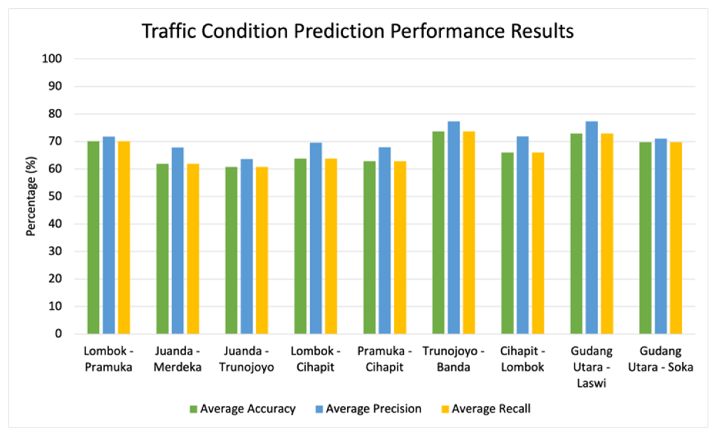
| Dataset | Average Accuracy (%) | Average Precision (%) | Average Recall (%) |
|---|---|---|---|
| Lombok-Pramuka | 70.05 | 71.77 | 70.05 |
| Juanda-Merdeka | 61.84 | 67.84 | 61.84 |
| Juanda-Trunojoyo | 60.78 | 63.64 | 60.78 |
| Lombok-Cihapit | 63.81 | 69.58 | 63.81 |
| Pramuka-Cihapit | 62.86 | 67.94 | 62.86 |
| Trunojoyo-Banda | 73.69 | 77.39 | 73.69 |
| Cihapit-Lombok | 66.00 | 71.82 | 66.00 |
| Gudang Utara-Laswi | 72.88 | 77.35 | 72.88 |
| Gudang Utara-Soka | 69.77 | 71.10 | 69.77 |
| Source | Destination | Vehicle Type | Traffic Condition | Weather Condition | Temperature | Humidity | Heterogeneity | Current Speed | Road Length | Compatibility |
|---|---|---|---|---|---|---|---|---|---|---|
| Cihapit | Banda | Car | 0 | Overcast clouds | 25.01 | 70 | 3 | 29 | 506 | 0 |
| Laswi | Gudang Utara | Car | 0 | Overcast clouds | 25.16 | 70 | 1 | 34 | 532 | 10 |
| Trunojoyo | Banda | Car | 0 | Overcast clouds | 24.99 | 70 | 3 | 25 | 446 | 0 |
| Seram_0 | Saparua_0 | Car | 2 | Overcast clouds | 25.01 | 70 | 1 | 27 | 273 | 10 |
| Pramuka | Lombok | Motorcycles | 0 | Overcast clouds | 25.01 | 70 | 1 | 36 | 877 | 0 |
| Cihapit | Pramuka | Motorcycles | 0 | Overcast clouds | 25.01 | 70 | 3 | 29 | 777 | 0 |
| Pramuka | Anggrek | Motorcycles | 0 | Overcast clouds | 25.1 | 70 | 4 | 29 | 320 | 0 |
| Seram_0 | Saparua_0 | Motorcycles | 2 | Overcast clouds | 25.01 | 70 | 1 | 27 | 273 | 0 |
| Source | Destination | Vehicle Type | Traffic Condition | Weather Condition | Temperature | Humidity | Heterogeneity | Travel Time | Road Length | Compatibility | RCV |
|---|---|---|---|---|---|---|---|---|---|---|---|
| Cihapit | Banda | Car | 0 | 0.5 | 0.25 | 0.5 | 0 | 0.99 | 0.49 | 0 | 0.33 |
| Laswi | Gudang Utara | Car | 0 | 0.5 | 0.252 | 0.5 | 1 | 0.99 | 0.47 | 10 | 10.54 |
| Trunojoyo | Banda | Car | 0 | 0.5 | 0.25 | 0.5 | 0.33 | 0.99 | 0.55 | 0 | 0.41 |
| Seram_0 | Saparua_0 | Car | 0.667 | 0.5 | 0.25 | 0.5 | 1 | 1 | 0.73 | 10 | 10.74 |
| Pramuka | Lombok | Motorcycles | 0 | 0.5 | 0.25 | 0.5 | 1 | 0.99 | 0.12 | 0 | 0.4 |
| Cihapit | Pramuka | Motorcycles | 0 | 0.5 | 0.25 | 0.5 | 1 | 0.99 | 0.22 | 0 | 0.42 |
| Pramuka | Anggrek | Motorcycles | 0 | 0.5 | 0.251 | 0.5 | 0.33 | 1 | 0.68 | 0 | 0.44 |
| Seram_0 | Saparua_0 | Motorcycles | 0.667 | 0.5 | 0.25 | 0.5 | 1 | 1 | 0.73 | 0 | 0.59 |
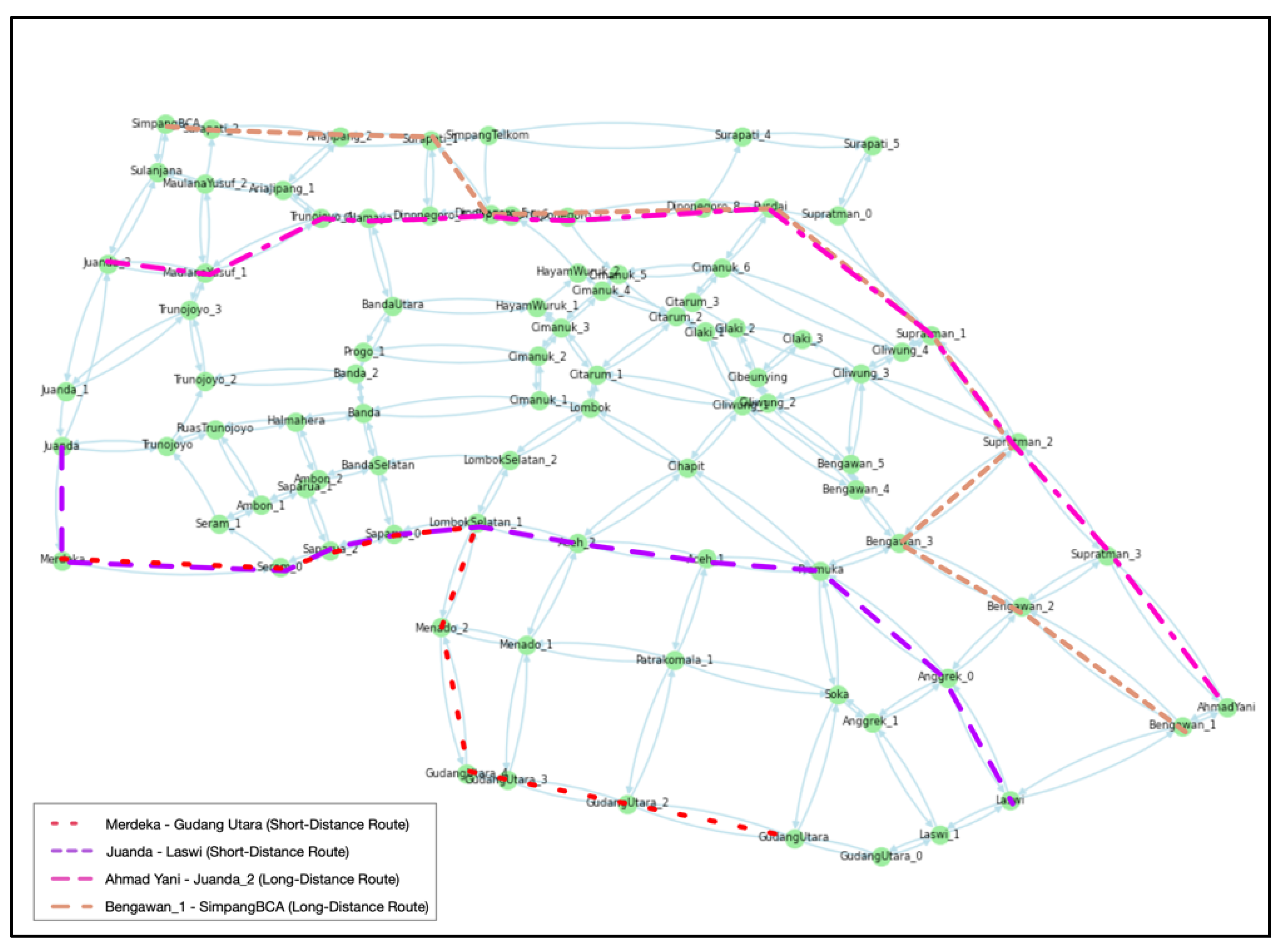
| Source | Destination | Distance Schemes | Distance (Meters) | Routes |
|---|---|---|---|---|
| Merdeka | GudangUtara | Short Distance | 2449 | Merdeka–Seram_0–Saparua_2–Saparua_0–LombokSelatan_1 – Menado_2–GudangUtara_4–GudangUtara_3–GudangUtara_2–GudangUtara |
| Juanda | Laswi | Short Distance | 3099 | Juanda–Merdeka–Seram_0–Saparua_2–Saparua_0–LombokSelatan_1–Aceh_2–Cihapit – Pramuka–Anggrek_0–Laswi |
| AhmadYani | Juanda_2 | Long Distance | 3624 | AhmadYani–Supratman_3–Supratman_2–Supratman_1–Pusdai – Diponegoro_7–Diponegoro_6–Diponegoro_5–Diponegoro_4–Cilamaya–Trunojoyo_4–MaulanaYusuf_1–Juanda_2 |
| Bengawan_1 | SimpangBCA | Long Distance | 3712 | Bengawan_1–Bengawan_2–Bengawan_3–Supratman_2–Supratman_1–Pusdai–Diponegoro_7–Diponegoro_6–Diponegoro_5–Surapati_1–AriaJipang_2–Surapati_2–SimpangBCA |
| Vehicle Type | Attributes Measurements | Routes |
|---|---|---|
| Car | RCV | Juanda-Merdeka-Seram_0-Saparua_2-Saparua_0-LombokSelatan_1-Aceh_2-Aceh_1-Pramuka-Anggrek_0-Laswi |
| Motorcycle | RCV | Juanda-Trunojoyo-RuasTrunojoyo-Halmahera-Banda-Cimanuk_1-Lombok-Cihapit-Pramuka-Anggrek_0-Laswi |
| Car/Motorcycle | Travel Distance | Juanda-Trunojoyo-RuasTrunojoyo-Halmahera-Banda-Cimanuk_1-Lombok-Cihapit-Pramuka-Anggrek_0-Laswi |
| Car/Motorcycle | Travel Time | Juanda-Merdeka-Seram_0-Saparua_2-Saparua_0-LombokSelatan_1-Aceh_2-Aceh_1-Pramuka-Anggrek_0-Laswi |
| Car/Motorcycle | Traffic Condition | Juanda-Juanda_2-MaulanaYusuf_1-Trunojoyo_4-Cilamaya-Diponegoro_4-Diponegoro_5-Diponegoro_8-Pusdai-Supratman_0-Supratman_1-Supratman_2-Bengawan_3-Pramuka-Anggrek_0-Laswi |
Publisher’s Note: MDPI stays neutral with regard to jurisdictional claims in published maps and institutional affiliations. |
© 2021 by the authors. Licensee MDPI, Basel, Switzerland. This article is an open access article distributed under the terms and conditions of the Creative Commons Attribution (CC BY) license (https://creativecommons.org/licenses/by/4.0/).
Share and Cite
Nasution, S.M.; Husni, E.; Kuspriyanto, K.; Yusuf, R.; Yahya, B.N. Contextual Route Recommendation System in Heterogeneous Traffic Flow. Sustainability 2021, 13, 13191. https://doi.org/10.3390/su132313191
Nasution SM, Husni E, Kuspriyanto K, Yusuf R, Yahya BN. Contextual Route Recommendation System in Heterogeneous Traffic Flow. Sustainability. 2021; 13(23):13191. https://doi.org/10.3390/su132313191
Chicago/Turabian StyleNasution, Surya Michrandi, Emir Husni, Kuspriyanto Kuspriyanto, Rahadian Yusuf, and Bernardo Nugroho Yahya. 2021. "Contextual Route Recommendation System in Heterogeneous Traffic Flow" Sustainability 13, no. 23: 13191. https://doi.org/10.3390/su132313191