The Measures of Accuracy of Claim Frequency Credibility Predictor

Abstract

Nowadays, the sustainability risks and opportunities start to affect strongly insurance companies in regard to the resulting additional variability of future values of variables taken into account in the decision processes. This is important especially in the era of sustainable non-life insurance promoting, among others, the use of ecological car engines or ecological systems of building heating. The fundamental issue in non-life insurance is to predict future claims (e.g., the aggregate value of claims or the number of claims for a single policy) in a heterogeneous portfolio of policies taking account of claim experience. For this purpose, the so-called credibility theory is used, which was initiated by the fundamental Bühlmann model modified to the Bühlmann–Straub model. Several modifications of the model have been proposed in the literature. One of them is the development of the relationship between the credibility models and statistical mixed models (e.g., linear mixed models) for longitudinal data. The article proposes the use of the parametric bootstrap algorithm to estimate measures of accuracy of the credibility predictor of the number of claims for a single policy taking into account new risk factors resulting from the emergence of green technologies on the considered market. The predictor is obtained for the model which belongs to the class of Generalised Linear Mixed Models (GLMMs) and which is a generalization of the Bülmann–Straub model. Additionally, the possibility of predicting the number of claims and the problem of the assessment of the prediction accuracy are presented based on a policy characterized by new green risk factor (hybrid motorcycle engine) not previously present in the portfolio. The paper presents the proposed methodology in a case study using real insurance data from the Polish market.

1. Introduction

Nowadays, the financial sector including the insurance industry strengthens its activities to promote and build sustainable economies and societies. The management of the sustainability risks, which takes into account both the asset and the liability side, but also a broader corporate perspective, becomes a very important issue (see [1]). The number of insurers who actively take into account different green factors in their risk assessment process is growing. The problem of including these factors in the prediction of different characteristics such as the total number of claims (e.g., [2]), crash severity (e.g., [3]) and accident risk (e.g., [4]) can play the crucial role from this perspective. A very basic feature of the non-life insurance portfolio of policies is its heterogeneity, which means that policies generate different values of claims. Consequently, charging each policy with the same pure premium (flat rate) is both unjust and uncompetitive. The pure premium is understood as the part of the gross premium intended to cover the current insurance risk of the policy. Therefore, insurers classify the portfolio into risk classes, and in each class the same value of pure premium is assigned to the grouped risks. In such a classification, various kinds of criteria are considered, simply referred to as risk factors. The nature of risk factors is important as they can be observable or unobservable. Observable factors (while signing an insurance contract) are described by the policyholder, e.g., the subject of the insurance, the policyholder and the geographical area. To be more precise, observable risk factors are categorical variables with a number of levels which divide the portfolio into risk classes (e.g., risks grouped by the age of the driver in automobile insurance). When it comes to unobservable factors, they describe items such as driving skills, drinking habits or the safety of the district in which the insured property is located. Unobservable factors can be approximated by observable factors. The area where the car is driven (unobservable) is usually assumed as the area where the car is registered (observable). A more complicated issue is to take into account the behavioral unobservable factors that reflect the inner traits or abilities of an individual policyholder.

This type of situation can be observed in (but of course is not limited to) real life problems resulting from taking into account new and ‘green’ technologies in the motor and property insurance. From our point of view, it is important for an insurance company to have a tool to deal with this kinds of problems in the age of climate change. In the era of sustainable development, new challenges arise related to green risk factors taken into account in the premium calculation (pricing) process. This can be broadly related to the guidelines included in the Principle of Sustainable Insurance document [5] presented for the first time in 2012. This global guide explains how to manage environmental, social and governance risks in the process of evaluating, defining and pricing non-life insurance risks. One of the problems is, in particular, the analysis of green risk factors which were not present in the premium calculation process before. For example—the engine type, which is the basic factor in automobile insurance. Currently, insurers reward hybrid or electric cars, which are considered more environmentally friendly. Another example is property insurance and the type of home heating. Therefore, there is a problem of the inclusion of the indicated risk factors in statistical models without historical data. Hence, we will propose the specific way to take into account this situation in the process of pure premium prediction.

In order to calculate the pure premium for the single policy in heterogenous portfolio, traditionally the credibility theory is applied, first proposed in [6]. In that theory, the pure premium for single ith policy, corresponding to the value of claims or the number of claims, is predicted for the next period taking the data from previous periods (the history of claims). The classic Bühlmann model from [6] defines so-called credibility predictor as the weighted average of prior portfolio mean ($\mu$) and the mean of claim experience for each ith policy (${\overline{Z}}_i$): $z_i{\overline{Z}}_i+(1-z_i)\mu$, where $z_i\in [0,1]$ denotes the credibility factor. The strong assumption is that the number of policies is constant in each period of the analysis. The Bühlmann–Straub model proposed in [7] allows for the variability of the number of policies over time. In both models the pure premium is viewed as the random variable being a function of a random parameter $\mathsf{\Theta }$ representing the unobservable risk factor of the individual policy and the distribution of $\mathsf{\Theta }$ describes the variation of this factor across the whole portfolio. The models presented in both papers were then generalized in many different ways, e.g., [8]. This article considers the development of the Bühlmann–Straub model towards a regression approach, where risk factors are included in the credibility predictor. In [9] the author proposes the linear trend credibility model. As the parameter $\mathsf{\Theta }$ is regarded as the random variable the mixed models approach to credibility prediction is adopted. In [10] authors provide examples of the credibility predictor by the use of Hierarchical Generalised Linear Models (HGLMs), further developed in e.g., [11,12] or [13]. In turn, the paper [14] provides the detailed derivation of the exact formula of predictors corresponding to different credibility models, including Bühlmann–Straub model, under particular linear mixed models (LMMs). The other topics connected with mixed models which belong to the GLMM class are studied in [15]. Authors present the so-called limited fluctuation credibility, where the predictor strongly depends on the sample size, the distribution of covariates and the link function. The GLMM is also considered in [16], where its application is presented for an analysis of longitudinal claims data by generalizing the normal assumption in Bühlmann–Straub model to Poisson and negative binomial distributions. The Poisson claim frequency, but in the form of Poisson mixtures (not as the GLMM), is also discussed in [17] assuming time-varying random effects and the frequency risks dependent on the latent individual factor corresponding to, e.g., the behavioral risk factors. These behavioral factors in credibility prediction can be analyzed in the case of the access to telematic data too. Then, the premium is calculated in the usage-based system, for instance in automobile insurance (by using GPS tracking in the car). The Poisson frequency claim models are discussed in this context by several authors, see [18,19,20]. Typically, in credibility models of frequency the accuracy of prediction is measured by the mean squared error (MSE), see [21]. There is also an alternative of using an expectation of a loss function measuring the discrepancy between real and predicted values (as considered in [22]) but in this case the loss function corresponds to the specific assumed distribution of the variable of interest. In this paper we will propose using different accuracy measures applicable for any prediction problem and its bootstrap estimator.

The aims of the paper cover the following issues. We will propose:

• The procedure in premium prediction taking into account some completely new risk factors (for which realizations of the response variable are not observed);
• Use of two accuracy measures applicable for any prediction problem based on the quantiles of absolute prediction errors;
• The parametric bootstrap estimators of the accuracy measures of the considered credibility predictor.

This paper is organized as follows. Section 2 presents the theoretical foundations of the credibility theory, in particular—the credibility predictor with emphasis on so far not observed risk factors which can result from sustainable insurance principles. In Section 3, a case is discussed of the claim frequency credibility predictor in the GLMM approach. Section 4 proposes estimators of the measures of accuracy in claim frequency prediction together with a full parametric bootstrap algorithm. The application of the method based on real data is presented in Section 5. The paper ends with a discussion.

2. The Background of Bühlmann–Straub Model

Generally, longitudinal data allows to take into account not only the spatial correlation between observations and the spatial correlation between the considered variables (observed in the case of cross-sectional data) but also changes in time of the variable of interest and then prediction for future periods. In credibility theory, which in under consideration, the idea is to predict the future premium (understood here as the future number of claims) for the single policy taking into account the historical data. That is why we will model the longitudinal data: it gives the possibility to take into account both dimensions—time and space—and increase the prediction accuracy due to the complex information on the phenomenon.

Let the population size of all policies (covering all combinations of risk factors, including green ones, of the insurer’s interest) be denoted by K. Let the size of the set of policies present in the current insurer’s portfolio be denoted by n, where $n\le K$. Let us also assume that longitudinal data on the policies from periods $t=1,\dots ,T$ are available but not necessarily balanced—it is not assumed that the data for the particular policy are observed in all T periods. Hence, the number of all observations is smaller than or equal to $nT$. What is important is that the insurer can be interested in the prediction for the future period and the policy covering the combinations of risk factors, including green ones, not observed in the available dataset.

In such a case the credibility theory could be applied, see [6,21]. The pure premium for the ith policy is defined there as the conditional mean:

$${\P }_i({\mathsf{\Theta }}_i)=E\left[Z_{i,T+1}\right|{\mathsf{\Theta }}_i],$$

(1)

where ${\mathsf{\Theta }}_i$ is the random variable representing the individual unobservable risk factor—the risk profile. In turn, $Z_{i,T+1}$ corresponding to the ith individual policy ($i=1,\dots ,K$) in period $T+1$ is the aggregate value of claims. It is assumed that these values are observed in periods $t=1,\dots ,T$ but not necessarily in all of them (unbalanced longitudinal data are considered), which makes it possible to measure the individual factor ${\mathsf{\Theta }}_i$ but for $i=1,\dots n$. However, in the insurance practice both ${\P }_i({\mathsf{\Theta }}_i)$ and ${\mathsf{\Theta }}_i$ are unknown, so there is a need to predict the value of ${\P }_i({\mathsf{\Theta }}_i)$. Let the predictor of ${\P }_i({\mathsf{\Theta }}_i)$ be denoted by $\widehat{{\P }_i({\mathsf{\Theta }}_i)}$. Nowadays, in lines of businesses such as automobile or homeowner insurance, insurers collect mass portfolios of risks. In their databases, detailed information is stored about the policies. This can be cross-sectional data, but often longitudinal data are available. This means that the portfolio of policies is observed during several periods, mostly on a yearly basis. Because of the fact that each policy can be renewed (usually on an annual basis), it is possible to analyze the claim history for each risk and apply the statistical model to compute the value of $\widehat{{\P }_i({\mathsf{\Theta }}_i)}$.

Let us start from the fundamental Bühlmann–Straub model presented in [7] and assume for the current portfolio (of size n) and for T periods. Let us assume that conditionally, for a given ${\mathsf{\Theta }}_i$, random variables $Z_{i,t}$ are independent and

$$E(Z_{i,t}|{\mathsf{\Theta }}_i)=\mu ({\mathsf{\Theta }}_i),$$

(2)

$$Var(Z_{i,t}|{\mathsf{\Theta }}_i)={\sigma }^2({\mathsf{\Theta }}_i),$$

(3)

where $\mu ({\mathsf{\Theta }}_i)$ is the individual risk premium, ${\sigma }^2({\mathsf{\Theta }}_i)$ is the variance within an individual risk, $i=1,\dots ,n$ and $t=1,\dots ,T+1$. Let us consider the following predictor of (1), which is a linear combination of past observations of the aggregate value of claims (c.f. [21]):

$$\widehat{{\P }_i({\mathsf{\Theta }}_i)}=a_{i0}+\sum _{t=1}^T{a}_{it}{Z}_{i,t}.$$

(4)

Let the parameters $a_{i0},\dots ,a_{iT}$, as discussed in [16], be estimated by minimizing the quadratic loss function: $L=E[{({\P }_i({\mathsf{\Theta }}_i)-a_{i0}-{\sum }_{t=1}^T{a}_{it}{Z}_{it})}^2]$. Then, the credibility predictor (4) takes the following form:

$$\widehat{{\P }_i({\mathsf{\Theta }}_i)}=z_i\overline{Z_i}+(1-z_i)\mu ,$$

(5)

where $z_i$ is the unknown credibility factor $z_i$ ranging from 0 to 1, ${\overline{Z}}_i=T^{-1}{\sum }_{t=1}^T{Z}_{i,t}$ is the average of historical claims for a single ith risk and $\mu$ is the overall mean in the current portfolio.

Predictor (5) is a function of the model unknown parameters. To obtain its empirical (estimated) version, the parameters must be replaced by their estimates. In the actuarial practice, the parameters of the Bühlmann–Straub model are usually estimated using the method of moments. However, in [14] the authors develop the link between the general formula of the Bühlmann–Straub model and the LMM for longitudinal data with fixed effects corresponding to the observable risk factors and random effects representing the individual risk profile. This makes it possible to estimate the model parameters using the maximum likelihood and the restricted maximum likelihood methods, which are usually used in this class of models. A drawback of using the LMM is the normality assumption of the response variable. Considering insurance data, which are usually right-skewed or discrete (claim frequency), a specific LMM has to be extended to the GLMM, see [23]. The GLMM no longer requires the normality assumption and can be adapted to distributions from the exponential family, such as the Poisson and the Gamma distributions. What is more, the approach presented in this section does not cover the case of prediction for new (including green) risk factors which the insurer would like to take into account, but which are not observed in the current portfolio.

3. Credibility Predictor of Claim Frequency

Claim frequency plays an important role in the calculation of the pure premium or, e.g., in motor insurance for the bonus-malus systems, see [24,25,26]. In frequency modeling it is usually assumed that the number of claims $N_{it},i=1,\dots ,n,t=1,\dots ,T+1$ follows a conditional Poisson distribution, where n is the size of the observed risk portfolio. This is why the credibility premium understood as $E\left[N_{i,T+1}\right|{\mathsf{\Theta }}_i]$ is often under consideration. In [16] the authors extend the LMM approach from [14] to the GLMM for the case of the Poisson distribution and derive a new formula of the credibility predictor (5) but for the observed ith risk factor. Consequently, the results presented below take additional account of new, including green, risk factors which were not present in the premium calculation process before (i.e., for policies indexed by $i=n+1,\dots ,K$). It is of special importance in the case of challenges resulting from the sustainable approach in the management in insurance companies.

Considering the claim frequency credibility predictor, let the number of claims be expressed as:

$$N_{it}|{\mathsf{\Theta }}_i\sim Poisson({\lambda }_0{\mathsf{\Theta }}_i),$$

(6)

where $i=1,\dots ,K$ (for all risk factors, including those not present in the current portfolio), $t=1,\dots ,T+1$ (for all periods including the future one), ${\lambda }_0$ is an unknown parameter and ${\mathsf{\Theta }}_i$ is an unobservable risk factor. The GLMM corresponding to Bühlmann–Straub model is described as follows:

$$E\left[N_{it}\right|{\mathsf{\Theta }}_i]=exp({\beta }_0+u_i),$$

(7)

where ${\beta }_0$ is the unknown fixed effect in the portfolio (the same for all policies) and $u_i$ represents normally distributed random effects with $E\left[u_i\right]=0$ and $Var\left[u_i\right]={\sigma }_u^2$. Hence, considering (7), ${\lambda }_0$ and ${\mathsf{\Theta }}_i$ in (6) can be written as ${\lambda }_0=exp({\beta }_0)$ and ${\mathsf{\Theta }}_i=exp(u_i)$, respectively. Under the GLMM, the credibility predictor will be given by:

$$\widehat{{\P }_i({\mathsf{\Theta }}_i)}={\widehat{N}}_{i,T+1}=\left\{\begin{array}{ccc}{z}_i\overline{N_i}+(1-z_i){\lambda }_0& for& i=1,\dots ,n\\ {\lambda }_0& for& i=n+1,\dots ,K.\end{array}\right.$$

(8)

The credibility factor here is $z_i=\frac{T}{\frac{1}{{\widehat{\nu }}_i}+T}$, where ${\nu }_i=Var(exp(u_i))$. Using the  moment-generating function of the number of claims N for Poisson distribution  $M_N(x)=E[exp(xN)]=exp(\lambda (exp(x)-1)$, it is possible to compute ${\nu }_i=exp(2{\sigma }_u^2)-exp({\sigma }_u^2)$. Of course it is possible to consider different distribution than the conditional Poisson distribution assumed in in (6), e.g., zero-inflated Poisson (ZIP) or negative-binomial and different model than (7), but then it will not correspond to the classic Bühlmann–Straub model but rather to its modification. On the other hand, in the case of a misspecification of the model the predictor can be biased and it can influence its accuracy as well.

Like predictor (8), predictor (5) depends on the model unknown parameters. To obtain the empirical (estimated) version of (8) they should be replaced by their estimates. The analysis presented herein makes use of the restricted maximum likelihood method, which is widely used in the case of the GLMM. What is also important, using the empirical version of (8) for policies not present in the current risk portfolio (i.e., for $i=n+1,\dots ,K$), the unpredictable random effects are not taken into account.

4. Bootstrap Estimators of Prediction Accuracy Measures for Claim Frequency

This section deals with the problem of prediction accuracy estimation, which is not considered in [16]. Although random effects for the risk factors not present in the insurer’s current portfolio, including those resulting from the emergence of green technologies, cannot be taken into consideration at the prediction stage (see (8)), their variability can be taken into account in the estimation of prediction accuracy. Let the prediction error for the ith policy, where $i=1,2,\dots ,K$, be denoted by $U_{i,T+1}={\widehat{N}}_{i,T+1}-N_{i,T+1}$. What is more, the new prediction accuracy measures (given by (11) and (12)) are proposed as alternative to the $MSE$, and their estimators (see (16) and (17)) are presented. The statement seems justified that their usage should be preferred to the $MSE$, because the $MSE$ is the mean of squared prediction errors whose distribution is strongly, positively skewed (see Figure 1). Let us consider the following prediction accuracy measures.

Firstly, the Mean Squared Error ($MSE$) is defined as

$$MSE({\widehat{N}}_{i,T+1})=E(U_{i,T+1}^2)$$

(9)

and the Root Mean Squared Error (RMSE) is given by:

$$RMSE({\widehat{N}}_{i,T+1})=\sqrt{MSE({\widehat{N}}_{i,T+1})}.$$

(10)

Secondly, for the problem under consideration, the Quantile of Absolute Prediction Errors ($QAPE$), originally proposed in [27] for small area prediction problems under the LMM and then used in [28] for the problem of prediction of the total loss reserve under the Hierarchical General Linear Model (HGLM), can be modified to the following form:

$$QAP{E}_p({\widehat{N}}_{i,T+1})=inf\{x:P(|U_{i,T+1}|\le x)\le p\}.$$

(11)

This means that (11) is the quantile of order p of absolute prediction errors. It also means that at least p100% of realizations of absolute prediction errors for the ith risk factor are smaller than or equal to $QAP{E}_p({\widehat{N}}_{i,T+1})$.

Thirdly, for the problem under consideration, the Quantile of a Mixture of Absolute Prediction Errors ($QMAPE$), originally proposed in [27] for small area prediction problems under the LMM, can be written as follows:

$$QMAP{E}_p({({\widehat{N}}_{i,T+1})}_{i=1}^K)=inf\{x:\sum _{i=1}^{K}P(|U_{i,T+1}|\le x)\le Kp\}.$$

(12)

Hence, it is the pth quantile of the distribution of a mixture of absolute prediction errors $|U_{i,T+1}|$ with equal weights, where $i=1,2,\dots ,K$. This means that at least p100% of realizations of absolute prediction errors for all risk factors are smaller than or equal to $QMAP{E}_p({({\widehat{N}}_{i,T+1})}_{i=1}^K)$.

Let us introduce Algorithm 1, see [28,29,30], which will be used to estimate the prediction accuracy for the considered model, where the variability of random effects will be taken into account also for the risk factors not observed in the considered dataset.

Algorithm 1 The parametric bootstrap algorithm

1: Based on observations of $N_{i,t}$ and the grouping variable defining the risk factors ($i=1,2,\dots ,n$; $t=1,2,\dots ,T$), estimate parameters of model (6) given by ${\beta }_0$ and ${\sigma }_u^2$ to obtain ${\widehat{\beta }}_0$ and ${\widehat{\sigma }}_u^2$. 2: for$b=1$ to B do 3:     generate realizations $N_{i,t}^{*(b)}$ of $N_{i,t}$ ($t=1,2,\dots ,T+1$; $i=1,2,\dots ,K$) under model (6) where ${\beta }_0$ and ${\sigma }_u^2$ are replaced by ${\widehat{\beta }}_0$ and ${\widehat{\sigma }}_u^2$, 4:     obtain estimates ${\widehat{\beta }}_0^{*(b)}$ and ${\widehat{\sigma }}_u^{2*(b)}$ using $N_{i,t}^{*(b)}$ ($i=1,2,\dots ,n$; $t=1,2,\dots ,T$), 5:     compute a bootstrap realization of the predictor ${\widehat{N}}_{i,T+1}$, see (8), denoted by ${\widehat{N}}_{i,T+1}^{*(b)}$, where $i=1,\dots ,K$ and parameters ${\beta }_0$ and ${\sigma }_u^2$ are replaced with estimates ${\widehat{\beta }}_0^{*(b)}$ and ${\widehat{\sigma }}_u^{2*(b)}$, 6:     compute bootstrap realizations of prediction error $U_{i,T+1}$ denoted by $u_{i,T+1}^{*}$ and for the bth iteration given by: $$u_{i,T+1}^{*(b)}={\widehat{N}}_{i,T+1}^{*(b)}-N_{i,T+1}^{*(b)},$$ (13) where $i=1,2,\dots ,K$. 7: end for 8: Compute the parametric bootstrap estimators of prediction accuracy measures: $$\widehat{MSE}({\widehat{N}}_{i,T+1})=B^{-1}\sum _{b=1}^B{u}_{i,T+1}^{*{(b)}^2},$$ (14) $$\widehat{RMSE}({\widehat{N}}_{i,T+1})=\sqrt{\widehat{MSE}({\widehat{N}}_{i,T+1})},$$ (15) $${\widehat{QAPE}}_p({\widehat{N}}_{i,T+1})=Q_p\left((|u_{i,T+1}^{*(b)}{|)}_{b=1}^B\right),$$ (16) $${\widehat{QMAPE}}_p\left({({\widehat{N}}_{i,T+1})}_{i=1}^K\right)=Q_p\left(((|u_{i,T+1}^{*(b)}{|)}_{b=1}^B{)}_{i=1}^K\right),$$ (17) where $Q_p(.)$ is the quantile of order p.

If the considered predictor is based on a different distribution and different model than that assumed in (6) and (7), then the bootstrap algorithm presented in this section should be modified taking into account the appropriate new assumptions.

5. The Case Study Based on Longitudinal Portfolio

The aim of this section is to apply the presented methodology to real data problem resulting from the sustainable insurance principles—the prediction of the number of claims and the estimation of accuracy for a green factor not present in the current portfolio. Considerations are based on a motorcycle dataset taken from a Polish insurance company. The data have a longitudinal structure and contain information from years 2007–2010 on 24 different risk factors. Every risk factor describes the insured vehicle according to:

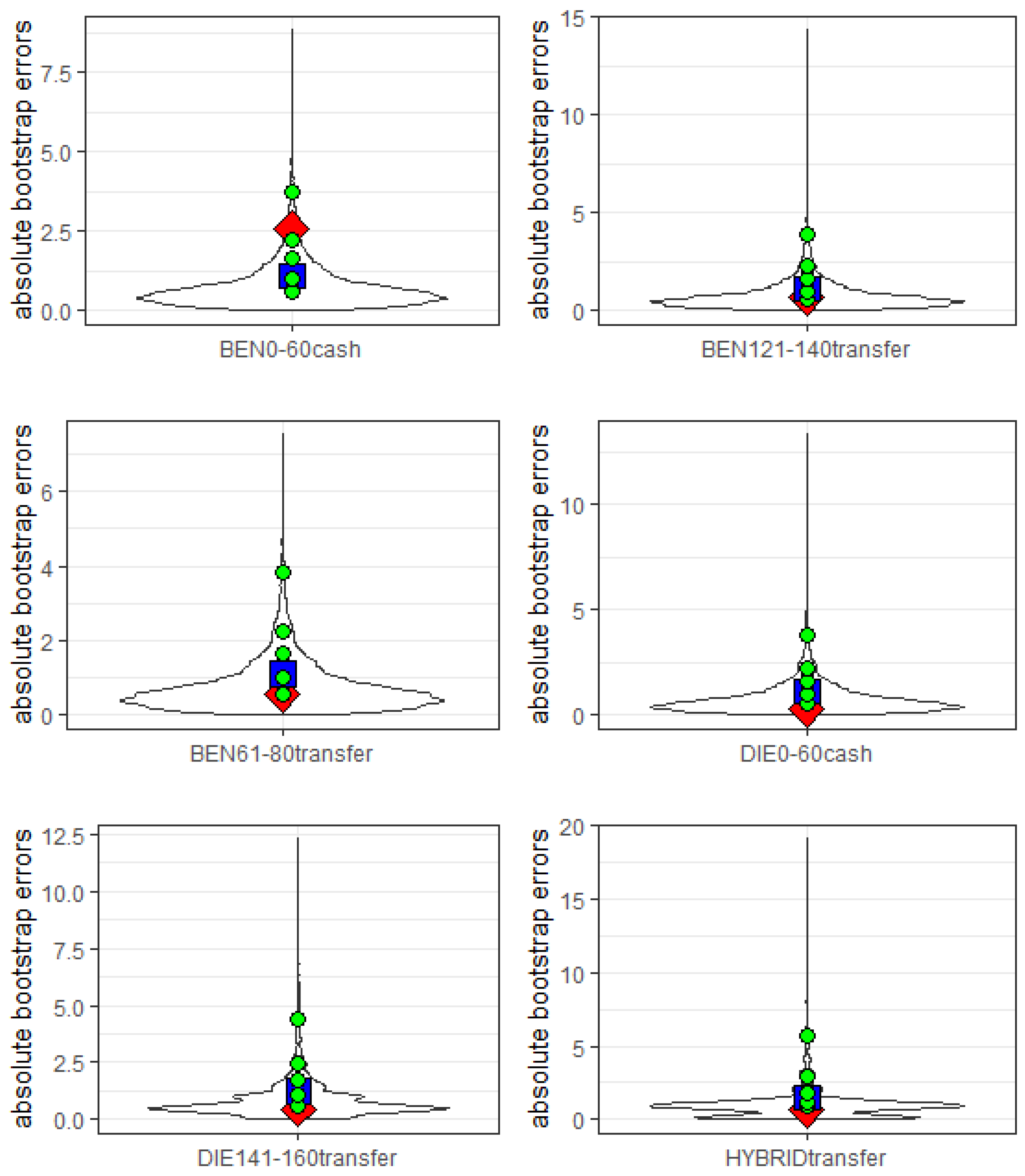
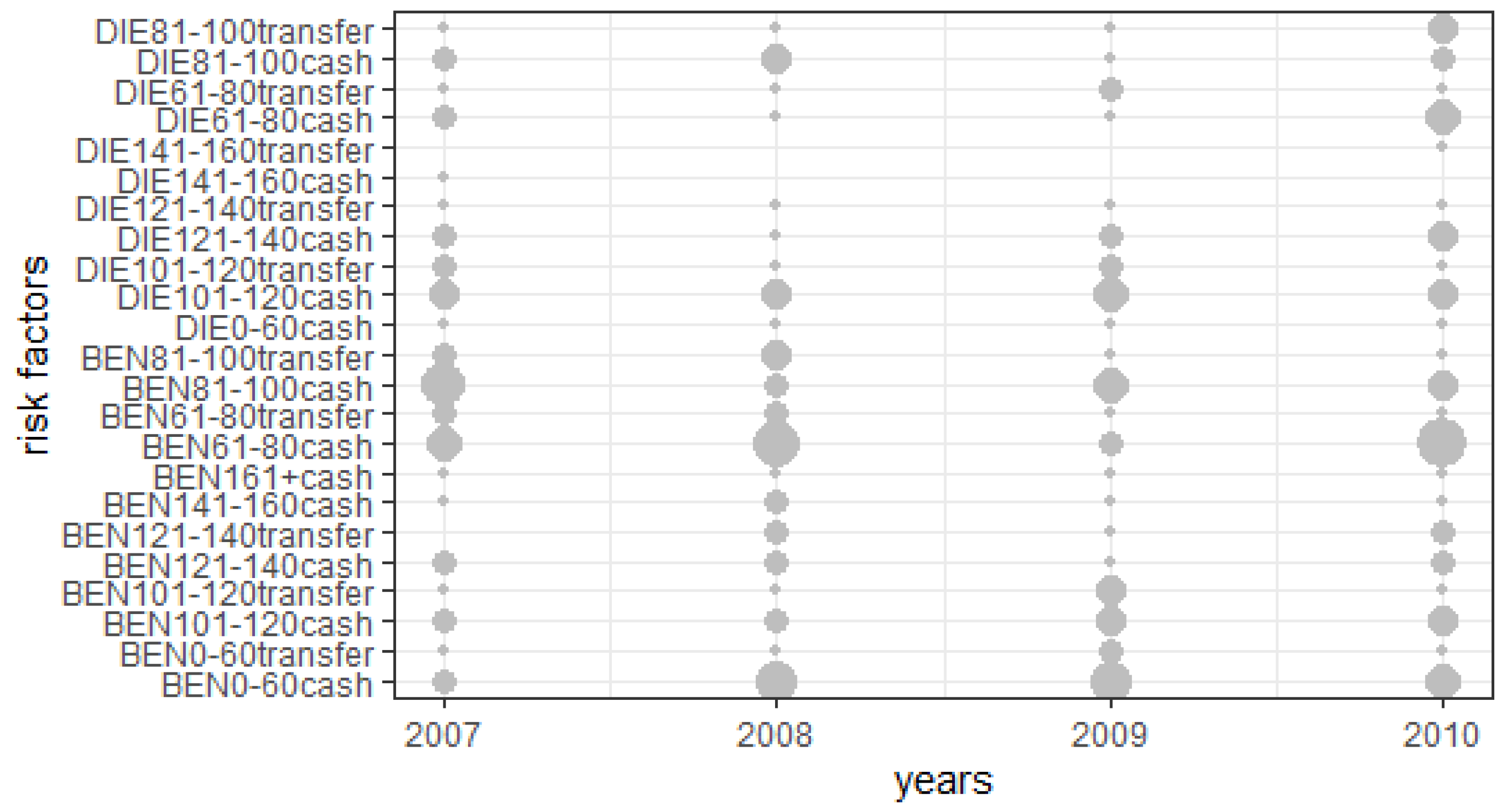
• The type of the engine—benzine (BEN), diesel (DIE), hybrid (HYBRID);
• The power range—0–60, 61–80, 81–100, 101–120, 121–140, 141–160, 160+;
• The type of payment—cash, transfer.

One unobserved green factor is assumed—$HYBRIDtransfer$, which means that we are interested in a policy paid by bank transfer for a motorcycle with a hybrid engine. Of course additional unobserved factors could be considered as well, for example hybrid type of engine for a policy paid by cash, but the methodology to be used will remain the same.

The variable of response is the number of claims of a single policy observed in every year. Relevant information is given in Figure 2. The empirical distribution presented in

Table 1. Empirical distribution of the number of claims in the portfolio.

Number of Claims	0	1	2	3	4	5	6	7
number of policies	41	23	11	5	2	1	1	1
fraction of policies	0.482	0.271	0.128	0.059	0.024	0.012	0.012	0.012

clearly demonstrates a strong positive asymmetry.

The aim is to compute the values of predictors for the year 2011, based on (8), and assess the prediction accuracy, based on (15) and our proposals: (16) and (17), mainly for $HYBRIDtransfer$, for which no past data are available but also for other risk factors. What is important is that the presentation of the results will not be limited to the values of the predictors and estimates of accuracy measures. The distributions of the parametric bootstrap absolute errors (see (13)) will also be presented, which is especially important due to the strong positive asymmetry of prediction errors and to the fact that the values of the variable of interest are natural (not real) numbers. The results will be presented using violin plots including the density function estimator with a mirror effect. The violin plot is more informative than a boxplot, e.g., because it makes it possible to show the multimodality of data and, additionally, to present outliers more clearly than in the case of a histogram. Showing the multimodality of the distribution may be important especially in the considered case of prediction errors computed as differences between the forecasts (which are real numbers) and the realizations of the variable of interest (which are natural numbers). What is more, the multimodality of the distribution is the additional argument in favor of using the quantiles (i.e., the $QAPE$ and $QMAPE$) instead of the mean (i.e., the $MSE$) to describe the distribution of prediction errors or at least its central tendency.

In the first step of the analysis, the values of the predictors of the number of claims are computed separately for all risk factors—they vary from $0.26$ to $3.73$ (see

Table 2. Values of the predictors and estimators of prediction accuracy measures for all risk factors.

Statistic	Value
${min}_{i=1,\dots ,K}{\widehat{N}}_{i,T+1}-{max}_{i=1,\dots ,K}{\widehat{N}}_{i,T+1}$	0.26–3.73
${min}_{i=1,\dots ,K}\widehat{RMSE}({\widehat{N}}_{i,T+1})-{max}_{i=1,\dots ,K}\widehat{RMSE}({\widehat{N}}_{i,T+1})$	1.06–1.50
${\widehat{QMAPE}}_{0.5}\left({({\widehat{N}}_{i,T+1})}_{i=1}^K\right)$	0.60
${\widehat{QMAPE}}_{0.75}\left({({\widehat{N}}_{i,T+1})}_{i=1}^K\right)$	1.01
${\widehat{QMAPE}}_{0.9}\left({({\widehat{N}}_{i,T+1})}_{i=1}^K\right)$	1.66
${\widehat{QMAPE}}_{0.95}\left({({\widehat{N}}_{i,T+1})}_{i=1}^K\right)$	2.27
${\widehat{QMAPE}}_{0.99}\left({({\widehat{N}}_{i,T+1})}_{i=1}^K\right)$	3.92

) including the predicted value for the $HYBRIDtransfer$ risk factor of $0.65$ (see

Table 3. Values of the predictor and estimators of prediction accuracy measures for $HYBRIDtransfer$ risk factor.

Statistic	Value
${\widehat{N}}_{i,T+1}$	0.65
$\widehat{RMSE}({\widehat{N}}_{i,T+1})$	1.50
${\widehat{QAPE}}_{0.5}({\widehat{N}}_{i,T+1})$	0.89
${\widehat{QAPE}}_{0.75}({\widehat{N}}_{i,T+1})$	1.18
${\widehat{QAPE}}_{0.9}({\widehat{N}}_{i,T+1})$	1.86
${\widehat{QAPE}}_{0.95}({\widehat{N}}_{i,T+1})$	2.92
${\widehat{QAPE}}_{0.99}({\widehat{N}}_{i,T+1})$	5.69

). Then, the bootstrap algorithm is run for all risk factors for the year 2011. The distributions of the bootstrap absolute prediction errors for six arbitrarily chosen risk factors (out of 24) are presented in Figure 1. Estimates of $RMSE$ (see (15)) for all risk factors are between 1.06 and 1.50 (see Table 2) including the value for the $HYBRIDtransfer$ risk factor of $1.50$ (see Table 3). However, all of the distributions have a very strong positive asymmetry with many outliers-the highest value of the absolute bootstrap error, ca. 19, is observed for the $HYBRIDtransfer$ risk factor. The strong positive asymmetry implies that the mean of squared errors (i.e., the $MSE$) and the $RMSE$ should be replaced with different accuracy measures. The proposal is to use the $QAPE$ estimators denoted by green circles in Figure 1. For example, the $QAPE$ estimate for order $p=0.99$ for the $HYBRIDtransfer$ risk factor (the right bottom corner of Figure 1, see also Table 3) equals $5.69$. Hence, it is estimated that at least 99% of absolute prediction errors for the $HYBRIDtransfer$ risk factor are smaller than or equal to $5.69$ and at least 1% of absolute prediction errors for the $HYBRIDtransfer$ risk factor are greater than or equal to $5.69$. It is the highest value of the $QAPE$ estimate of order $p=0.99$ for the risk factors presented in Figure 1.

In the second step of the analysis all the absolute bootstrap errors computed for all of the 24 risk factors (not only the six risk factors presented in Figure 1) are taken into account. These values are presented in Figure 3. Hence, the distribution can be interpreted as the distribution of a mixture of the bootstrap absolute prediction errors for all risk factors with equal weights. Then, quantiles of these values are computed, as defined in (17), denoted by green lines in Figure 3. For example, the estimate of $QMAPE$ for order $p=0.99$ equals $3.92$ (see also Table 2). Hence, it is estimated that at least 99% of absolute prediction errors for all risk factors are smaller than or equal to $3.92$ and at least 1% of absolute prediction errors for all risk factors are greater than or equal to $3.92$.

In the last step of the analysis, the estimates of $QAPE$s-quantiles of bootstrap absolute prediction errors for the $HYBRIDtransfer$ risk factor are compared to the estimates of $QMAPE$s-quantiles of bootstrap absolute prediction errors for all risk factors. In Figure 4 estimates of $QAPE$s are presented as green circles, while the estimated $QMAPE$s are represented by green lines; these results are also presented in Table 2 and Table 3. What is important, for the same order of the quantile, $QAPE$s are greater than respective $QMAPE$s. For example, it is estimated that the median of absolute prediction errors for the $HYBRIDtransfer$ risk factor equals $0.89$, while for all risk factors it is $0.60$. It is not surprising because $QAPE$s are estimated for the unobserved green risk factor $HYBRIDtransfer$, while the $QMAPE$ is computed for all risk factors, only one of which has not been observed.

Summing up, the presented methodology enables prediction of claim counts and estimation of the prediction accuracy for risk factors even not present in the current portfolio. It is crucial due to the necessity of extending the decision-making process in the insurance company to so far not taken into account information on new green technologies (in our case: hybrid motorcycle engine). In addition, it makes it possible to compare the prediction accuracy with other individual risk factors and also with the whole risk portfolio.

6. Discussion

The development of sustainable insurance leads to new challenges which influence management processes in insurance companies. The paper deals with the problem of taking account of new risk factors resulting from the emergence of green technologies in the premium pricing process, cf. [4]. The GLMM extension of the commonly used Bühlmann–Straub model is studied. The problem of the prediction of the number of claims is extended, comparing with [16], by estimation of the prediction accuracy. New measures are presented too—they make it possible not only to assess the prediction accuracy but also to compare the prediction accuracy for new green risk factors with the accuracy of the whole risk portfolio. They are also not limited to the assessment of the average prediction accuracy but enable a description of the whole distribution of absolute prediction errors. The authors believe that the considered issue of assessing the prediction accuracy for risk factors currently not present in the portfolio is crucial for the effective conduct of the insurance business in accordance with the principles of sustainable development. The theoretical considerations presented herein are supported by an application based on a real longitudinal dataset of policies sold by a Polish insurance company.

Of course the proposed bootstrap estimation procedure is not limited to just dealing with new risk factors classified as “green”. The presented methodology can be used for any new risk factors including new distribution channels, regions or customer groups. In practice, a large percentage of changes in (non-life) insurance data concerns information related to the climate change and the premium level adaptation to new technologies. Basically, incorporating “green” risk factors in modeling is not the same as reducing the pure premium in terms of data prediction. It is only the premium better adjustment for the future along with an increase in the number of observed periods in the sample. What is more, based on our results insurers can take into account not only the value of the predictor but also the distribution of the predictions errors, which can lead to more effective business decisions. Generally, values of the predictors and higher estimated prediction errors in the case of unobserved risk factors do not have to justify the reduction of the premium at least until new observations of claims are available. However, the insurers can take into account not only their own historical data but also wider information from the entire market.

References

1. Gatzert, N.; Reichel, P.; Zitzmann, A. Sustainability risks & opportunities in the insurance industry. ZVersWiss 2020, 109, 311–331. [Google Scholar]
2. Gómez-Déniz, E.; Calderín-Ojeda, E. A Priori Ratemaking Selection Using Multivariate Regression Models Allowing Different Coverages in Auto Insurance. Risks 2021, 9, 137. [Google Scholar] [CrossRef]
3. Shiran, G.; Imaninasab, R.; Khayamim, R. Crash Severity Analysis of Highways Based on Multinomial Logistic Regression Model, Decision Tree Techniques, and Artificial Neural Network: A Modeling Comparison. Sustainability 2021, 13, 5670. [Google Scholar] [CrossRef]
4. Huang, J.S.; Wang, K.C. Are Green Car Drivers Friendly Drivers? A Study Of Taiwan’S Automobile Insurance Market. J. Risk Insur. 2019, 86, 103–119. [Google Scholar]
5. United Nations Environment Programme Finance Initiative. Principles for Sustainable Insurance; UNEP FI: Gland, Switzerland, 2012. [Google Scholar]
6. Bühlmann, H. Experience rating and credibility. Astin Bull. J. IAA 1967, 4, 199–207. [Google Scholar] [CrossRef] [Green Version]
7. Bühlmann, H.; Straub, E. Glaubwürdigkeit für schadensätze. Bull. Swiss Assoc. Actuar. 1967, 70, 111–133. [Google Scholar]
8. Jewell, W.S. Credible means are exact Bayesian for exponential families. ASTIN Bull. J. IAA 1974, 8, 77–90. [Google Scholar] [CrossRef] [Green Version]
9. Hachemeister, C.A. Credibility for regression models with application to trend. In Proceedings of the Credibility, Theory and Applications, Berkeley Actuarial Research Conference on Credibility, Berkley, CA, USA, 19–21 September 1974; pp. 129–163. [Google Scholar]
10. Nelder, J.A.; Verrall, R.J. Credibility theory and generalized linear models. ASTIN Bull. J. IAA 1997, 27, 71–82. [Google Scholar] [CrossRef] [Green Version]
11. Ohlsson, E.; Johansson, B. Exact credibility and Tweedie models. ASTIN Bull. J. IAA 2006, 36, 121–133. [Google Scholar] [CrossRef] [Green Version]
12. Ohlsson, E. Combining generalized linear models and credibility models in practice. Scand. Actuar. J. 2008, 2008, 301–314. [Google Scholar] [CrossRef]
13. Rosenlund, S. Credibility pseudo-estimators. Scand. Actuar. J. 2019, 2018, 770–791. [Google Scholar] [CrossRef]
14. Frees, E.W.; Young, V.R.; Luo, Y. A longitudinal data analysis interpretation of credibility models. Insur. Math. Econ. 1999, 24, 229–247. [Google Scholar] [CrossRef]
15. Garrido, J.; Zhou, J. Full credibility with generalized linear and mixed models. ASTIN Bull. J. IAA 2009, 39, 61–80. [Google Scholar] [CrossRef] [Green Version]
16. Xie, Y.T.; Li, Z.X.; Parsa, R.A. Extension and application of credibility models in predicting claim frequency. Math. Probl. Eng. 2018, 2018, 6250686. [Google Scholar] [CrossRef]
17. Pinquet, J. Poisson models with dynamic random effects and nonnegative credibilities per period. ASTIN Bull. J. IAA 2020, 50.2, 585–618. [Google Scholar] [CrossRef]
18. Denuit, M.; Montserrat, G.; Trufin, J. Multivariate credibility modelling for usage-based motor insurance pricing with behavioural data. Ann. Actuar. Sci. 2019, 13, 378–399. [Google Scholar] [CrossRef] [Green Version]
19. Gao, G.; Meng, S.; Wüthrich, M.V. Claims frequency modeling using telematics car driving data. Scand. Actuar. J. 2019, 2019, 143–162. [Google Scholar] [CrossRef]
20. Gao, G.; Wüthrich, M.V.; Yang, H. Evaluation of driving risk at different speeds. Insur. Math. Econ. 2019, 88, 108–119. [Google Scholar] [CrossRef]
21. Bühlmann, H.; Gisler, A. A Course in Credibility Theory and Its Applications; Springer: Berlin/Heidelberg, Germany, 2005. [Google Scholar]
22. Denuit, M.; Trufin, J. Generalization error for Tweedie models: Decomposition and error reduction with bagging. Eur. Actuar. J. 2021, 11, 325–331. [Google Scholar] [CrossRef]
23. Antonio, K.; Beirlant, J. Actuarial statistics with generalized linear mixed models. Insur. Math. Econ. 2007, 40, 58–76. [Google Scholar] [CrossRef]
24. Boucher, J.; Denuit, M. Fixed versus random effects in Poisson regression models for claim counts: A case study with motor insurance. Astin Bull. 2006, 36, 285–301. [Google Scholar] [CrossRef] [Green Version]
25. Boucher, J.P.; Guillén, M. A survey on models for panel count data with applications to insurance. RACSAM-Rev. Real Acad. Cienc. Exactas Fis. Nat. Ser. Mat. 2009, 103, 277–294. [Google Scholar] [CrossRef]
26. Boucher, J.P.; Inoussa, R. A posteriori ratemaking with panel data. ASTIN Bull. 2014, 44, 587–612. [Google Scholar] [CrossRef]
27. Żądło, T. On asymmetry of prediction errors in small area estimation. Stat. Transit. New Ser. 2017, 18, 413–432. [Google Scholar] [CrossRef] [Green Version]
28. Wolny-Dominiak, A.; Żądło, T. On bootstrap estimators of some prediction accuracy measures of loss reserves in a non-life insurance company. Commun.-Stat.-Simul. Comput. 2020. [Google Scholar] [CrossRef]
29. Flores-Agreda, D.; Cantoni, E. Bootstrap estimation of uncertainty in prediction for generalized linear mixed models. Comput. Stat. Data Anal. 2019, 130, 1–17. [Google Scholar] [CrossRef] [Green Version]
30. Żądło, T. On accuracy estimation using parametric bootstrap in small area prediction problems. J. Off. Stat. 2020, 36, 435–458. [Google Scholar] [CrossRef]
Figure 1. Distributions of absolute bootstrap errors for 6 arbitrary selected (out of 24) risk factors with Q A P E ^ p ( . ) of orders p = { 0.5 , 0.75 , 0.9 , 0.95 , 0.99 } denoted by green circles, R M S E ^ ( . ) denoted by blue square, and the value of the predictor denoted by red rhombus (all outliers are included).
Sustainability 13 11959 g001
Figure 2. The number of claims for every risk factor in years 2007–2010 presented as points. The size of points demonstrates the value of the number of claims from 0 to 7 on an increasing scale.
Sustainability 13 11959 g002
Figure 3. Joint distribution of absolute bootstrap errors for all risk factors with Q M A P E ^ p ( . ) of orders p = { 0.5 , 0.75 , 0.9 , 0.95 , 0.99 } denoted by green lines (all outliers are included).
Sustainability 13 11959 g003
Figure 4. Distribution of absolute bootstrap errors for HYBRIDtransfer risk factor with Q A P E ^ p ( . ) of orders p = { 0.5 , 0.75 , 0.9 , 0.95 , 0.99 } denoted by green circles, R M S E ^ ( . ) denoted by blue square, the value of the predictor denoted by red rhombus, and Q M A P E ^ p ( . ) s of orders p = { 0.5 , 0.75 , 0.9 , 0.95 , 0.99 } denoted by green lines (less than 1% of outliers are excluded, the maximum value not shown in the figure equals ca. 19).
Sustainability 13 11959 g004