1. Introduction
1.1. Background
The International Energy Agency has estimated about a 50% increase in the demand for energy in the buildings sector by 2060 [
1]. Buildings, as a sector, are accountable for around one-third of total global energy use [
2]. Several control strategies are being developed to improve the energy performance of buildings (of any functionality in the residential, commercial, municipal, and institutional sectors) [
3,
4]. Building automation, integrated with control strategies, enables the building owners and managers to achieve energy efficiency targets for green building ratings and standards [
5]. In addition, the operational efficiency of buildings can be improved by changing the occupants’ behavior and by developing improved energy control algorithms that consider active occupancy dynamics. Such considerations enable the building energy system (BES) to operate at an improved energy usage point without jeopardizing the safety and comfort of the occupants.
Energy modeling is a very important part of the building energy control design [
6,
7,
8,
9]. The development of a reliable and accurate building energy model is, thus, necessary in order to investigate the feasibility and performance of the energy control strategies. Reliability in the building energy model involves the inclusion of all the significant parameters in model development, and the achievement of a response that is as close in approximation as possible to real-time experiments or standardized empirical results [
10,
11,
12]. The American Society of Heating, Refrigerating and Air-Conditioning Engineers (ASHRAE), an intergovernmental organization headquartered in Georgia, the United States, enables the modelers and researchers to develop building energy simulation models using the test procedures laid out in the ANSI/ASHRAE Standard 140-2007 [
13].
1.2. Literature Survey
Building energy system models can be categorized as white-box, black-box, and grey-box energy models, depending upon the availability of the experimental data [
14,
15]. White-box models are purely theoretical models that involve mathematical formulations of the energy transfer processes occurring within the building under consideration. The physical elements, such as the building envelope (walls, roof, floor, etc.), and the windows, shades, etc., are considered as single-layered or multilayered elements for developing building energy models [
16,
17]. Single-layered modeling has been mostly used to develop energy control strategies for heating, ventilation, and air-conditioning (HVAC) [
18,
19,
20] and lighting systems [
21,
22].
The development of building energy models using multilayered construction elements improved the accuracy by taking into account the thickness, density, heat conductivity, and thermal capacity of each layer that constitutes a building element [
23,
24]. However, many studies report multilayer constructions that ignore the thermal air gaps within the construction elements. Control solutions developed for building energy systems, such as lighting, ventilation control, and blind control, etc., often become unstable when the system is simulated for a longer period of time [
25,
26]. A building energy model becomes unstable when excited by rapidly varying inputs and also because of unmodeled disturbances, such as outdoor environmental conditions, transient occupancy fluctuations, etc. This instability results in the occupants’ discomfort and high-energy consumption. Building energy simulation programs have been developed for building energy system model development and analysis. The procedure adopted by building energy simulation programs for design and model development is shown in
Figure 1 [
27].
In the conceptual design phase, building energy simulation programs assist in optimal designing and modeling in order to achieve a high level of comfort for the occupants. However, the assessment of the stability to variable inputs, and the interactions between the state variables and the input parameters, is not conducted. The problems of ineffective control that arise in the later phases of the detailed design phase, postconstruction phase, and the operation and control phases can be prevented by conducting stability and controllability tests at the conceptual design phase [
28]. The additional costs that are incurred during the maintenance and rectification of control problems at a later stage of the operation can, thus, be avoided.
The building energy system models developed so far use dynamic modeling and undergo simulations to test the detailed design, where the cost of error removal is high [
29,
30]. Such models have embedded conventional control techniques, such as on-off, PI, and PID control. As any particular building energy system is a MIMO system, identifying the factors responsible for the model’s instability and parametric uncontrollability becomes a very tedious exercise. Moreover, this may lead to losses during the post-commissioning and operation phase, as there exists a large number of influential parameters [
31]. Thus, during the design phase, it becomes imperative to conduct stability and controllability tests on the developed building energy system models and identify the extent of the state-input variable interactions (
Table 1).
1.3. Gaps Identified
Very little research has been conducted on the stability studies and controllability assessments of building energy system models. Counsell et al., 2011, developed a full-scale building energy model of a school in Scotland using the climate-adaptive building philosophy [
31]. Basic heat and mass transfer energy equations were used to develop a building energy model for a single zonal space. Mathematical expressions using ordinary differential equations governing the building space air temperature, lux-level, and CO
2 concentrations were developed.
Similar works are reported in [
31,
45], where building energy models were formulated as state-space equations. The structure and rank of the
CB+
sD matrix of the developed state-space model were observed in a root-locus analysis to determine the direction of the asymptotes and, hence, the stability. The effects of the outdoor parameters, such as the wind characteristics, temperature, and solar radiation, were not considered. The assessments were carried out for full-scale building energy system models, which increased the complexity of the developed building energy system model. The parameter of relative humidity was ignored.
The building energy models reported in the literature have been developed for assessing the energy performance of building energy systems, rather than for assessing the stability and controllability of the system against the servicing parameters, such as building space air temperature, air relative humidity, luminance, and indoor air quality. Moreover, building energy systems are MIMO systems with several energy transfer interactions occurring within and outside the system. Precise and computationally efficient building energy system models are required in order to effectively assess the controllability and stability of the servicing parameters. Some studies have used mechanical ventilation for controlling CO2 concentration levels only and have ignored the cooling aspect.
The present study aims to find potential solutions and explore answers to questions such as:
(Q1) In which step of building energy model development can one assess for variables in model simulation that can be controllable or not?
(Q2) How can the stability of a building energy system model be tested?
(Q3) How can we investigate both the stability and the controllability of an integrated building energy system model?
(Q4) What framework/approach should exist to investigate the input to state interaction for building energy system models?
1.4. Significant Contributions of the Paper
In this paper, the concepts of stability and controllability are investigated for the energy system models of building. The energy plant taken into consideration for this study is an HVAC system. Controllability assessment studies were conducted for a range of setpoint values. Passive energy control and comfort management strategies were not considered in this study. A methodology for conducting stability and controllability assessment tests on the building energy model is proposed using inverse dynamics input theory (IDIT) [
46,
47]. The present study extends the work published in [
23,
48]. The building energy system model is represented in state-space form in order to understand the interactions between the building space variables (both outdoor and indoor), such as air temperature, humidity, occupancy, and other causal thermal gains and state variables, such as the nodal temperatures of the building elements, HVAC heating/cooling load, and lighting system load.
A white-box single zonal mathematical building energy system model was developed in MATLAB/Simulink. Lumped capacitance (RC) network models were considered for the building construction elements, such as the walls, roof, etc. IDIT was adopted for the controllability assessment test because of its ability to study a MIMO system as a number of SISO systems with reduced complexity and less, or no, loss of information. The strategy developed in this paper characterizes the important properties of building energy systems through the analysis of the state-equation data (namely, the coefficient matrices A, B, C, and D using IDIT). Tracking the trajectory of how control variables are influenced by state variables for building energy system models may assist the building designers, energy control engineers, retrofitters, and managers in order to improve the procedure for developing energy control strategies for the building industry. A similar approach can be applied to low-, medium-, and high-thermal capacity buildings. As the input-to-state trajectory of the energy system variables can be assessed for stability and controllability, designers can be guided for both the slow and fast actuation of HVAC systems. The approach developed in this paper may also generate interest in conducting energy control research in order to assess the developed energy system models before developing and applying any energy control strategies.
The remainder of this paper is categorized as follows:
Section 2 introduces the basic concepts of the stability and controllability tests for a linear time-invariant state-space model;
Section 3 represents the methodology for analyzing the stability and assessing the controllability of the building energy system; the simulation results are presented in
Section 4 and
Section 5;
Section 7 discusses the results in detail and points out the limitations; and
Section 8 concludes the paper.
2. Concepts of Stability and Controllability
2.1. Stability
For a particular control model, stability is the most significant factor for analyzing the performance of a system. A system is said to be stable, for a particular interval of time, if the response, or output, of the system remains finite when it is excited by a set of finite inputs over the same time interval. In order to test a particular system model for stability, several testing criteria are available, depending on the nature and characteristics of the model. For LTI systems, the Nyquist stability and Routh’s stability criterions are usually used. For nonlinear and time-varying systems, such stability criteria do not apply [
49]. Lyapunov stability analysis is the most common method for the stability determination of non-LTI systems [
50].
A system is said to be unstable if, for a particular range of operations, the output tends to infinity for any one, or combination, of its input excitations. Mathematically, the stability of a system,
G(
t), can be defined as Equations (1) and (2).
If
then,
G(
t) is unstable for every value of time,
t.
Moreover, if
where ‘
K’ is the finite value, then,
G(
t) is stable for every value of time,
t, where
t0 = initial time.
For state-space systems, there are different concepts of stability, such as uniform stability (a more general way of defining stability), asymptotic stability (eigen values of the system matrix have negative real parts), and exponential stability (system response decaying exponentially towards zero as time approaches infinity). There are applications where a system can possess uniform asymptotic stability, depending upon the equilibrium and the zero-state point of the state-space system.
2.2. Controllability
Controllability exhibits the structural features of a dynamic system and is a characteristic property. The conditions on the controllability and stability often govern the control solution. For a state-space control system, rules exist for the conduct of controllability tests. An LTI system is described by Equations (3) and (4).
where
| A = System coefficient matrix |
| b = Input coefficient matrix |
| c = Output coefficient matrix |
| d = Input-output coupling matrix |
A system defined by Equations (3) and (4) is said to be controllable if there exists an input, , that enables the system to be transferred from an initial state, , to another state, , in a finite interval of time, . A system is said to be completely controllable if all of its initial states are controllable; otherwise, the system is said to be uncontrollable.
The solution of Equation (3) is:
assuming, without loss of generality, that
, the system is controllable if:
where
τ = Time variable.
From Equation (6), it can be observed that a system’s complete controllability depends on A and b and is independent of c and d. Equation (5) represents the system controllability of the pair (A, b). As per Equations (3)–(6), no constraint is imposed on the inputs or on the trajectory that the state should follow. This implies that a system could be controllable for a finite interval of time even if it is uncontrollable. Such a restriction does not enable the control plant to follow the control rules for a desired interval of time. However, if the system satisfies the controllability condition, then there can be no intrinsic limitation on the design of the control system for the plant. If the processing and the significant variables of the system model are maintained within the acceptable range, then it is immaterial whether the plant is completely controllable or not.
Practically, building energy systems are nonlinear in nature and small perturbations of A and b can cause an uncontrollable system to become controllable. For MIMO systems, a plant can achieve complete controllability if the number of control variables is increased. Moreover, for models with redundant state variables, an increase in the number of control variables can cause a controllable system to become uncontrollable. For a MIMO system, such as a building energy system, it is usually difficult to compute system controllability using Equation (6).
2.3. Realizing Stability through Root Locus Plots
The frequencies at which the system under study tends to reach towards infinity are regarded as poles, and the frequencies at which the system tends to reach towards the origin, or zero, are regarded as zeros of the system. The transfer function representation of a particular system helps in assessing its stability without having to solve the differential equation characterizing the system. For a linear system to be stable, all the poles of the transfer function must possess negative real parts, i.e., their position should be within the left half of the
s-plane. The performance of a particular system can be analyzed using the pole-zero plot or the root-locus plot. For a linear system, if the number of poles is greater than that of zeros, then that system is said to be a practically realizable system [
36].
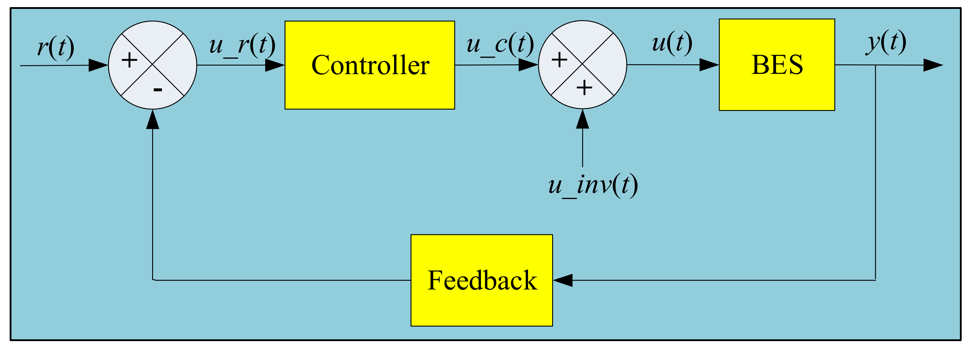
For a closed-loop MIMO system, such as a building energy system, the basic characteristic of the response is analyzed using the location of the closed-loop poles. Under situations of variable gain for the building energy system, the value of the gain at any instant in time depends on the position of the poles. It is, therefore, important to have knowledge of the trajectory of the closed-loop poles, as the gain is varied over the simulation period in the
s-plane. If the position of the poles remains the same after varying the gain value, then a compensator has to be added to achieve the desired results. The root-locus plots the roots of the characteristic equation for all values of a system parameter. A block diagram of a building energy system with a controller is shown in
Figure 2.
The closed-loop transfer function for the system shown in
Figure 2 is given as Equation (7).
where
| Y(s) = Laplace transform of actual output of the system, y(t) |
| R(s) = Laplace transform of input signal, r(t) |
| GC(s) = System transfer function of controller with u_r(t) as input and u_c(t) as output |
| GBES(s) = Building energy system’s transfer function under study with u(t) as input and y(t) as output |
| H(s) = Negative feedback signal |
| r(t) = Desired output |
| u_inv(t) = Dynamic inverse input and is defined as per the IDIT, given as Equation (8) |
The characteristic equation of the system is given as Equation (9):
by using the equality of angles and magnitudes for complex numbers,
where
n = 0, 1, 2, …
Equations (11) and (12) are called the angle and magnitude conditions, respectively. The closed-loop poles of the building energy system can be computed by evaluating s from the abovementioned equations. The locus of all such s-points in the complex s-plane is called the root locus.
3. Stability and Controllability Analysis of Building Energy Systems
After estimating and identifying the parameters of the building energy system model, it is crucial to analyze the performance of the model. Before developing the control strategies for building energy systems, it is imperative to conduct feasibility studies and tests on the building energy system model in order to set performance standards for model selection and evaluation. The set of the input and output parameters of energy systems used for the stability analysis and controllability assessment are shown in
Figure 3.
The primary aim of the developed HVAC system model is to regulate the building space air temperature and CO
2 concentration. This is to ensure the optimal air temperature for the comfort of the occupants, and the effective circulation of fresh air in and out of the building space. The outputs of an HVAC system, which are
TBS and
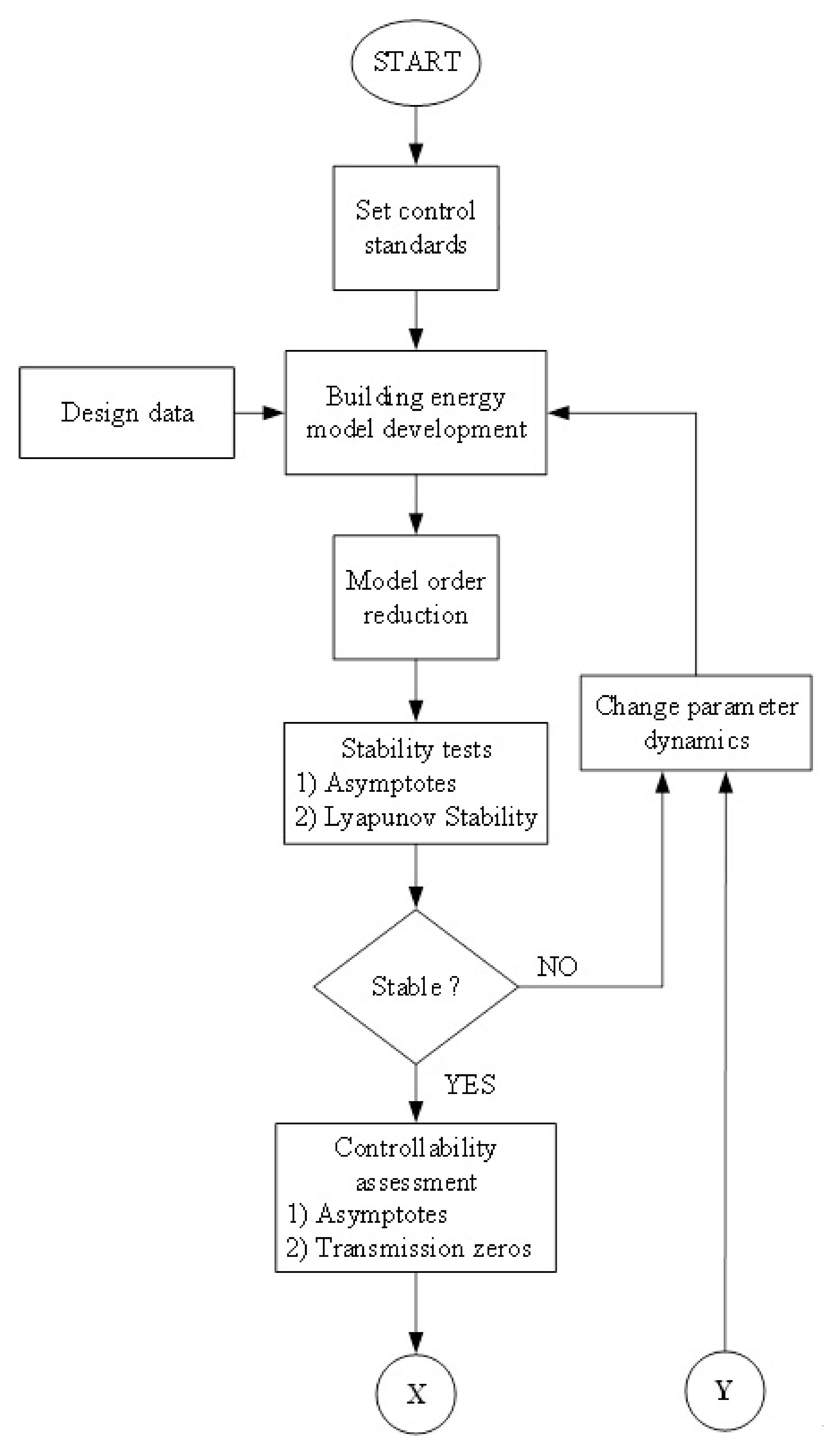
RHBS, are considered for the controllability analysis. A process flowchart of the strategy for the stability and controllability assessments followed in the present study is shown in
Figure 4. In the present study, the potential of the developed building energy system to be stabilized for the development of any energy control strategy is investigated by using the IDIT, which was developed for the aerospace industry [
31,
47].
The building energy system model developed in [
23,
26] is represented in state-space form as Equations (13) and (14):
where
| = Vector matrix of first-order derivatives of building energy system temperatures |
| X = Nodal temperature state-matrix |
| U = Building energy system’s temperature and HVAC load parameter vector |
| Y = Vector of TBS, building space temperature and RHBS, building space relative humidity |
| A = Building energy system model coefficient matrix |
| B = Vector matrix of building energy system model input coefficients |
| C = Vector matrix of output coefficients |
| D = Coupling matrix of input and output coefficients |
The parameters of building energy system models operate simultaneously in a designed control algorithm, and each parameter acts on an actuator to reach a desired setpoint value/level. The building energy system state-space model, as given in Equations (13) and (14), is converted into transfer function form as Equations (15)–(18):
where
| NP-Z = Numerator polynomial of G(s) after pole-zero cancellation |
| DP-Z = Denominator polynomial of G(s) after pole-zero cancellation. |
The poles of
G(
s) are the roots of
DP-Z(
s), which are the uncancelled eigen values of
A (substituting λ for
s), as in Equations (19) and (20):
and,
Equation (20) provides the internal system poles and, as there are pole-zero cancellations in computing G(s), Equation (20) provides the information on the input/output (external) stability of the system. Thus, for internal stability, all the eigen values of A must have negative real parts.
Transmission Zeros
For a linear-time-invariant system, state equations, representing a system, are equal in number to that of closed-loop poles. Transmission zeros are the states corresponding to the infinite poles of the system under study. Such poles are the asymptotes, or branches of the root loci, describing the system. The present study involves the control of the building space air temperature, relative humidity, CO
2 concentration, and lux level, and these parameters will be fed back into the system, i.e., the output of the feedback block of
Figure 2.
The inverse dynamics input,
u_inv(
t), enables the system poles to be positioned on top of system zeros, thereby making the states of the system controllable. This means that the closed-loop poles of the system are nothing but the open-loop zeros of the same system. The zeros are determined by the open-loop transfer function, given as Equation (21).
The transmission zeros for a model are determined by equating Equations (13) and (14) to zero, i.e.,
Equations (22) and (23) are written in matrix form as Equation (24).
The transmission zeros can then be finally determined by calculating the determinant of Equation (24):
4. Stability Analysis of Building Envelope Model
The state-space stability of the building envelope model is analyzed by observing the eigen values of the coefficient matrix,
A. The coefficient matrix for the building envelope, shown in
Figure 3, are given as Equations (26)–(30). The coefficient matrix for the outdoor wall is given as Equation (26):
where
AOW = the coefficient matrix for the outdoor wall state-space model of a building energy system.
A pole-zero plot for Equation (26) is shown as
Figure 5.
There are two poles for the outdoor wall model, as
AOW is of a two-by-two dimension. The poles of the outdoor wall state-space model are at -0.2408 and -0.0134. The poles of the outdoor wall state-space model lie on the left half of the pole-zero plane and, thus, the model is stable. Similarly, the coefficient matrices of the adjacent wall, roof, floor, and lobby wall are given as Equations (27)–(30), and the corresponding pole-zero plots are given as
Figure 6,
Figure 7,
Figure 8 and
Figure 9, respectively.
where
Aadjw = Coefficient matrix for adjacent wall building envelope model.
where
Aroof = Coefficient matrix for roof wall building envelope model.
where
Afloor = Coefficient matrix for floor wall building envelope model.
where
Alobby = Coefficient matrix for lobby wall building envelope model
The poles of the adjacent wall state-space model are at −1.9816, and −0.1102, whereas the poles of the roof state-space model are at −0.8157, and −0.0454.
The poles of the floor state-space model are at −1.1235, and −0.0625, whereas the poles of the lobby wall state-space model are at −0.9223, and −0.0272. Every pole of the system transfer functions for the construction elements lie in the negative half of the s-plane. This shows that the building envelope model is stable. Moreover, because of the absence of any pole-pairs on the s-plane, the system is completely stable and does not oscillate.
The coefficient matrix for the window state-space model is given as Equation (31):
where
Awin = Coefficient matrix for window state-space model of building energy system.
The pole-zero plot for the window state-space model, described as per Equation (31), is shown in
Figure 10.
There are two poles for the window model, as Awin is of a two-by-two dimension. The poles of the window state-space model lie on the left half of the pole-zero plane. The poles of the window state-space model are at −0.0884 and −0.1973. The position of these poles makes the window state-space model stable.
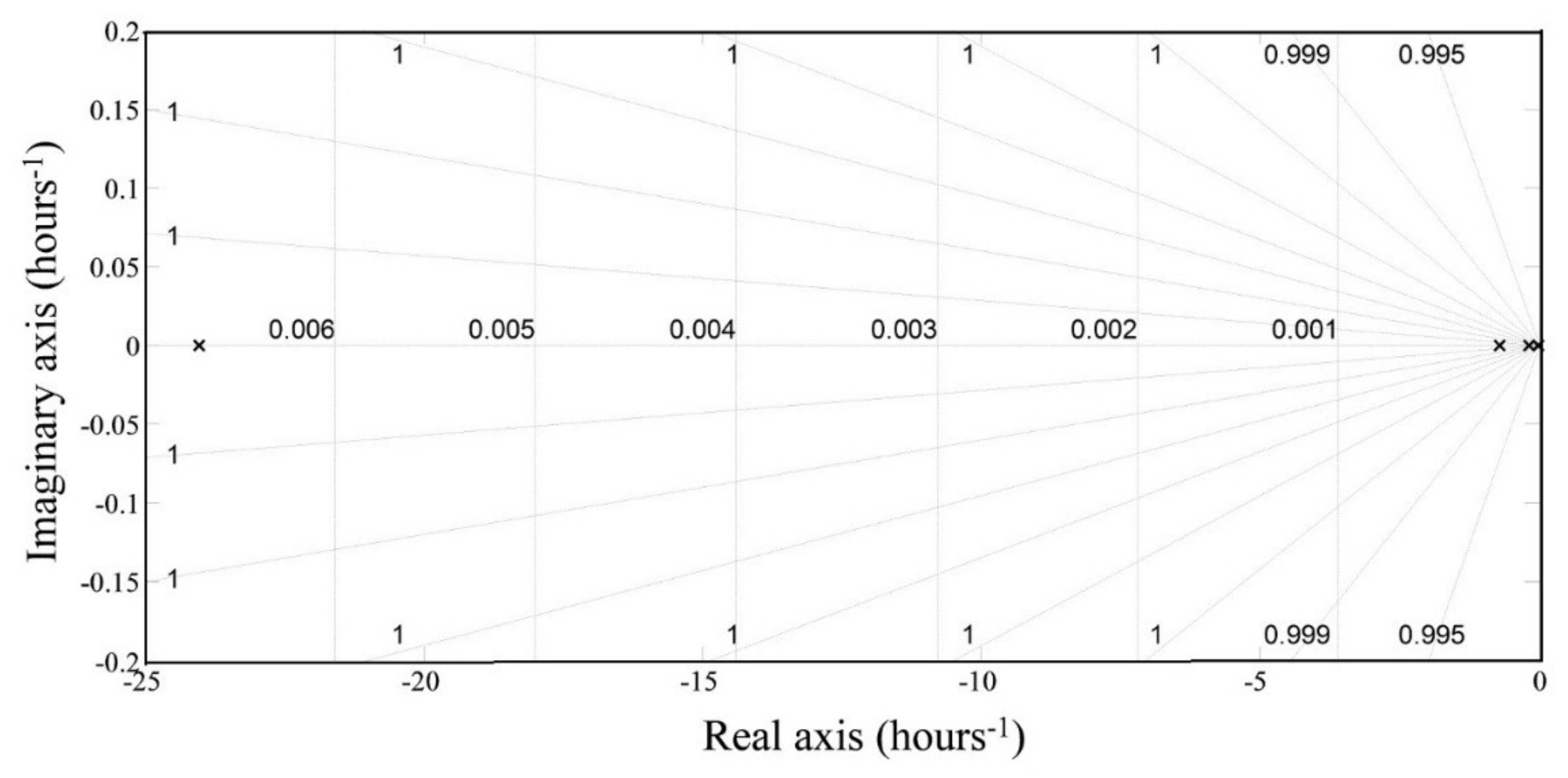
5. Stability Analysis of Building Space Model
The state-space stability of the building space model is analyzed by observing the eigen values of the coefficient matrix,
A. The coefficient matrix for the building space state-space model, (
ABS), is given as Equation (32).
Using the eigen values of Equation (32) and the
ABS of the building space model, then poles location is shown in
Figure 11.
There are four poles for the building space model, as ABS is of a four-by-four dimension. The poles of the building space model are at −0, −0.0001, −0.0002, and −0.0067. The poles of the building space model lie on the origin and on the left half of the pole-zero plane. There are three poles very close to the origin. These poles tend to make the building space model marginally stable.
6. Stability Analysis and Controllability Assessment of Building Space Model
A typical HVAC system is responsible for both the temperature and humidity control of the building space. With consideration given to all the building elements responsible for hygrothermal energy transfer processes within a building space, a full-order building energy system model has been developed.
6.1. Building Energy System Model
A virtual test setup was developed in MATLAB/Simulink and a thermal resistor-capacitor network was used for the building energy system model representation. A schematic of the test setup is shown in
Figure 12. The parameter values of the test setup are given in
Appendix A.
In order to assess the complete stability and controllability of the building energy system, energy transfer equations governing the development of the model have been reproduced as Equation (33):
where
| = Rate of heat transfer due to causal factors of solar radiation, lighting, occupancy, and appliances in the building space/zone, W/m2 |
| = Rate of heat transfer due to structural elements of the building space, such as windows, etc., W/m2 |
| = Rate of heat transfer due to ventilation and/or circulation of air within the building space, W/m2 |
| = Heat transfer rate of heating/cooling from the plant, W/m2 |
| = Density of air in the building space, kg/m3 |
| = Specific volume of air in the building space, m3/kg |
| = Specific heat capacity of air in the building space, kJ/kg-K |
The rate of heat transfer due to causal factors is given as Equation (34):
where
= Rate of heat transfer due to solar radiation through windows, W/m
2 and is given by Equation (35):
where
| = Absorptivity constant |
| = Transmissivity of the window |
| = Effective surface area of window, m2 |
| = Solar radiation incident on the window surface, W/m2 |
and,
= Amount of power converted into heat due to lighting luminaires installed in the building space, W/m
2, and is given by Equation (36):
where
| = Proportion of lighting power contributing to the heat gains |
| = Wattage rating of the luminaires, W |
and,
= Heat transfer rate due to occupants of the building space, W/m
2, and is given by Equation (37):
where
| = Number of occupants |
| = Occupants heat gain rate (calculated as per ASHRAE principles), W, |
and,
= Heat transfer due to appliances, such as computers/desktops, laptops, and other peripherals operating in the building space, W/m
2, and is given by Equation (38):
where
| = Number of appliances operating within the building space |
| = Heat gain produced by the appliances (calculated as per ASHRAE principles), W. |
The rate of heat transfer ventilation and the circulation of air within the building space is given as Equation (39):
where
= Air change due to internal thermal forces, W/m
2, and is given by Equation (40):
and
= Air change due to external thermal forces, W/m
2, and is given by Equation (41).
and
= Air change due to infiltration through the building space, W/m
2, and is given by Equation (42).
and
= Air change due to forced/mechanical ventilation through the building space, W/m
2, and is given by Equation (43).
The differential equation for the amount of water vapor in the air of the building space is given as Equation (44).
where
| = Building space humidity gain, kg/s |
| = Internal humidity gain, kg/s |
| = Loss of humidity due to thermal buoyancy, kg/s, and is given as Equation (45). |
and
= Humidity loss by wind pressure, kg/s and is given by Equation (46).
and
= Humidity loss by natural air change rate, kg/s and is given by Equation (47).
and
= Humidity loss by mechanical/forced ventilation, kg/s and is given by Equation (48).
Equations (34)–(49) of the building energy system are represented linearly in a matrix form as Equations (49) and (50).
where
D = Vector of disturbances.
Small amplitude perturbation is studied by analyzing the dynamic behavior of the building energy system under study using the state-space model of Equation (49) and Equation (50). It is to be noted that these equations represent a steady-state equilibrium condition.
A,
B,
C, and
f represent the time-invariant matrices of the constants. The state vectors of the complete building energy system model under study are given as Equations (51)–(53).
The stability and controllability of the system were assessed using the
CB matrix and IDIT [
32]. The
CB stability matrix of the system is given as Equation (54) and simplified as Equation (55).
From the equation, it can be observed that there exists a cross-coupling between temperature and humidity. This is achieved because of mechanical ventilation, (b12), which affects both the humidity and the temperature values of the building space. The primary cause for this cross-coupling is due to water evaporation in the building space, which adds to the hygrothermal losses. Such losses, however, are difficult to quantify and are modeled as disturbances to the developed building energy system model.
Term b12 of the CB matrix represents a cross-coupling of the temperature parameter that, in the present study, is equal to the difference in the building space and outdoor temperatures. The magnitude of the b12 parameter changes with seasonal variations. Smaller differences in the building space and outdoor temperature yield smaller b12 values, which represent the summer seasonal condition. This means that the developed building energy system model can employ a conventional PID-controlled HVAC system. During winter conditions, the temperature difference will be large and, hence, b12 will be a larger value. Such scenarios will demand the modeling of an external parameter for the mechanical ventilation of the PID-controlled HVAC system.
6.2. Simulation Results
In the present study, the developed building energy system is a multi-input multi-output system. Asymptotes for such a system can be represented using the
CB matrix’s eigen values. The asymptotes for the developed building energy system model are given as Equation (56).
where
g = Gain value which can be regulated globally throughout the system
σ = Scalar gain value.
Equations (55) and (56) can be combined as follows:
The above equation yields the values of s-, which are the asymptotes of the building energy system model’s output parameters, viz., the building space temperature and humidity, which can be expressed as follows:
where
s1 represents the asymptote for the building space air temperature, and the negative sign indicates that the transient response of the temperature will be stable and there will not be any oscillations in the temperature parameter to reach its steady-state value, whereas
s2 becomes positive under unconditioned situations where the building space humidity levels are greater than that of the outdoor level. Under such instances, the transient humidity response becomes unstable as well as uncontrollable, as
s2 aligns to the positive of the s-plane. This is occurring because of the term,
b22, of the
CB matrix. In order to make the transient humidity response stable and controllable, the
s2 asymptote needs to be realigned. This can be achieved by allotting a negative value to the gain,
σ2. This condition is shown in the
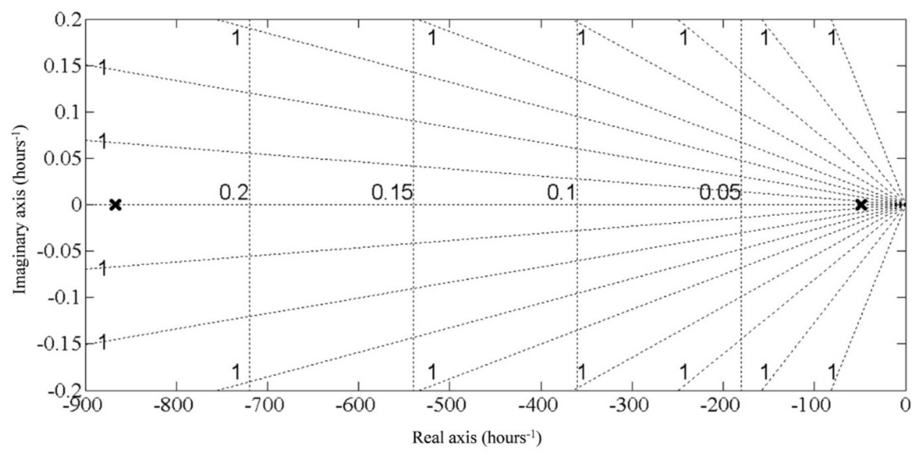
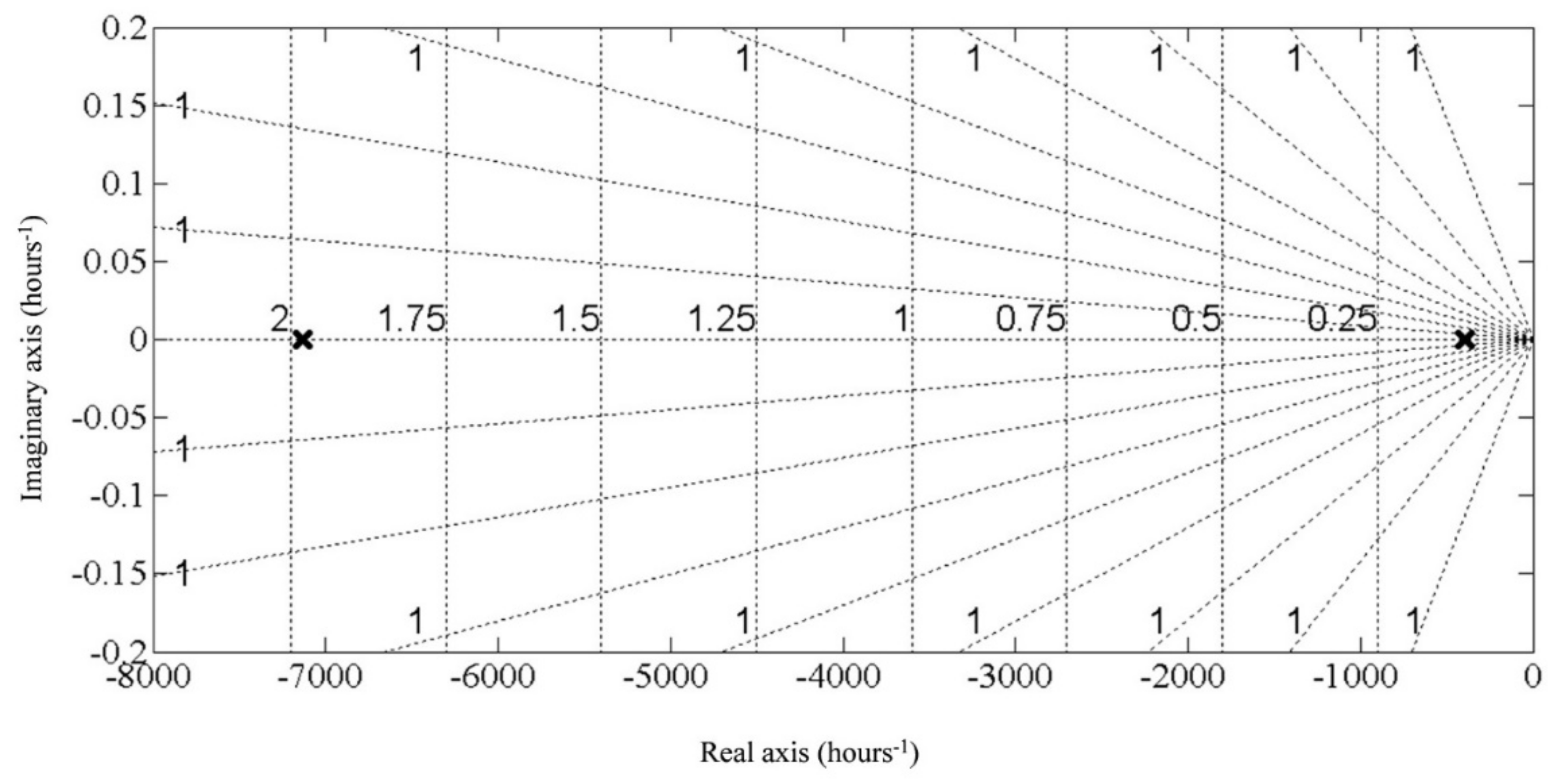
s-plane and is given in
Figure 13.
The asymptotes of
Figure 13 are the function of the temperature and humidity differences between the outdoor environment and the building space. Moreover, as the asymptotes are not at an angle, with respect to the real axis, and are negatively aligned towards the left half of the plane, the variation in the operating temperature and humidity levels will not affect the controllability of the developed building energy system model. If we consider the region to the right of the imaginary axis, the response can be seen to be increasing as the time increases. That means that no defined final state of the building energy system can be reached as time,
t →
.
By considering all of the asymptotes for all of the parameters in the developed building energy system model, total stability can be assessed using the TZ matrix of an MIMO system. The TZ matrix represents the transmission zeros of an MIMO system and is given as Equation (63).
On performing reductions, the TZ matrix is remodified as Equation (64).
The transmission zeros computed by solving the determinant of Equation (64) are given as Equation (65).
The transmission zeros are given as Equations (66) and (67).
From the above equations, it can be seen that s2 and s3 are negatively aligned on an s-plane, thereby signifying the total stability of the developed building energy system model. As is evident from Equations (66) and (67), the transmission zeros are independent of outdoor environmental variations, such as temperature, humidity, and solar radiation. The transmission zeros vary with the variations in the thermophysical properties of the building construction elements and the thermal transmittance of the internal and external thermal mass of the building space.
7. Discussion and Limitations of the Present Study
The control strategies developed for building energy systems become unstable for a particular range of operations when the system is simulated for a longer period of time, resulting in occupant discomfort and high-energy consumption. The present study applies conventional stability tests on the developed building energy system model and assesses the state-control trajectory of the model against the parameters of the building space air temperature, relative humidity, lux level, and CO2 concentration.
The methodology for conducting the stability and controllability assessment tests on the building energy model is presented. The developed testing methodology assists in determining the feasibility of an energy control strategy that can be applied in order to enhance the energy performance of a building. The state-space building energy system enables the representation of the interactions between the building space variables (both outdoor and indoor), such as air temperature, humidity, occupancy, and other causal thermal gains and state variables, such as the nodal temperatures of the building elements, HVAC heating/cooling load, and the lighting system load. Gaining knowledge about such interactions enables the modeler to determine the extent to which state trajectories can be controlled by varying the input parameters to the building energy system.
The thermal transmittance of the multilayered construction elements is reciprocal of the corresponding R-value. For lower costs and lower emissions, the U-value is kept low, adhering to the building regulations and codes. Applying this to the developed building energy system model yields low-thermal-capacity multilayered construction elements making up the building space. This increases the reaction speed to the control inputs as the location of zero is a function of the heat transmitted through the fabric and the heat stored in it. Thus, the thermal capacity of the construction element is significant for responsive control.
The present study does not consider the seasonal variations on the building energy system model. The controllability assessment approach presented in this paper may need modification when applied to climate-adaptive building energy systems. However, the approach for conducting the stability tests may remain identical. Passive heating and cooling strategies need to be explored and included, and the air gaps in the multilayered construction elements have been ignored.
The present study did not consider the effects of thermal bridging in the building walls. In order to develop a model with improved sophistication, the effective thermal transmittance of the building envelope can be calculated using available methods, such as ASTM Standard C1363, the effective area approach, the weighted average method, and thermographic survey. An accurate thermal model needs to be considered in order to make the assessment approach widely applicable. The present study does not demonstrate a controllability assessment for other parametric outputs, such as heating/cooling power, lighting load, energy usage, etc.
8. Conclusions
Because of the presence of one stable transmission zero during building space air temperature control (without humidity control), conventional single-input single-output (SISO) controllers, such as the PI controller, are adequate for controlling the building space air temperature without giving consideration to humidity. A stable and controllable building energy system model can now be used to develop control strategies for the effective management of the energy control and occupant comfort of buildings.
The discussions outlined above shall not always be true in the case of an unconditioned passive building. This is because the passive design of a building makes use of the thermal mass and capacity of the construction elements for satisfying the cooling load and also for thermal storage. Applying the current controllability assessment approach will yield sluggish and slow responses for the temperature and humidity parameters. However, this shall not be a concern, as the present study focuses primarily on conditioned building energy system modeling, where the PID-controlled HVAC system exists for the humidity and temperature control of the building space.
Investigating the stability and controllability of building energy system models may also help in reducing the validation errors. Though the approach reported in this paper may be used for building energy system model verification, the determination as to what degree the developed model actually represents the physical real world can be explored in the future. The approaches and techniques used for the uncertainty analysis of system variables can be clubbed with the developed IDIT approach, and the results obtained from the same can be analyzed. Such an approach may strengthen the verification, validation, and uncertainty analysis of building energy system models. This, in turn, shall lead to savings of both time and money.


