Article

Effects of Expansionary Monetary Policy on Agricultural Commodities Market

by
Klára Čermáková
* and
Eduardo Aguiar Henrique Filho
Department of Economics, Faculty of Economics, Prague University of Economics and Business, 130 67 Prague, Czech Republic
*
Author to whom correspondence should be addressed.
Sustainability 2021, 13(16), 9317; https://doi.org/10.3390/su13169317
Submission received: 11 July 2021 / Revised: 31 July 2021 / Accepted: 10 August 2021 / Published: 19 August 2021
(This article belongs to the Collection New Trends in Corporate Finance for Sustainability)

Abstract

:
Agricultural commodities experienced a rise in prices during the first decade of the 2000s. The literature shows that the monetary policies adopted by developed economies can influence practically all economic indicators of developing markets. This paper aims to evaluate the effect of selected monetary policy measures on the prices of three selected agricultural commodities: soy, corn and sugar. Secondly, the study analyzes the price formation of these commodities during a period of expansionary monetary policy, in order to better understand how they are influenced by unconventional instruments. The central hypothesis is that the excessive liquidity created by the FED spills over to emerging economies, boosting investment and consumption there and, lastly, causing a commodity cycle. Our data (January 2000–December 2019) support this hypothesis and prove that expansionary monetary policy is capable of impacting agricultural commodities’ prices, but by different channels, due to the specificities of each commodity. The fact that people have more capital due to the credit obtained from loans seems to influence the price of sugar; soy is highly influenced by exchange rates of emerging markets, and corn is not very responsive to the used variables, which might be due to the high production rates of this commodity in the U.S. and the protectionist policies adopted by the government.

1. Introduction

Agriculture is no less globalized than other sectors of the economy. Agricultural commodities are no longer traded by a merchant in a galleon, but by contracts traded at high speed in various exchanges.
The opulence of commodity exchanges and trading firms are not necessarily the same for producers and agriculture-dependent countries. According to the United Nations [1], historically, the lower the countries’ income, the larger its agricultural share in GDP. In 1980, the share of agriculture in GDP was almost two times higher in low-income countries than in middle-income ones, and it was almost three times higher in 2010. From 1980 to 2010, the agricultural share in GDP for high-income countries decreased by 66%, and, for low-income ones, by 31%. In Africa, 81% of exports were commodities in 2010, and 56% were commodities for Latin America and the Caribbean for the same year. Technology in agribusiness is thriving, helping developing economies to gain competitiveness and allowing them to pursue more complex activities. Promising study fields for agriculture include genetic engineering, data mining for agricultural, artificial intelligence for plantations, blockchain to help in the supply chain of agricultural goods, and an endless variation of technology for various purposes, from fighting pests to forecasting the nutritional information of each individual crop.
The world experienced a significant boom in commodities consumption from 2000 to 2014, largely stimulated by emerging markets’ increased consumption. The new Chinese middle class is hungry in many senses—for food, investments, housing, leisure, and education. Brazilians experienced a credit expansion in their country that increased consumption as well. The world craves for commodities, and this demand is expressed through prices; the question to be answered is “are commodity prices shocked by monetary stimulus?” and “How do commodities differ in sensitivity to monetary stimulus?” This paper evaluates whether the formation of prices for three selected commodities (soy, corn and sugar) is influenced by monetary policy and, additionally, how this relationship unfolds during a period of monetary expansion. The basic idea is that the FED is able to create commodity cycles in emerging economies by producing a scenario of excessive liquidity. The first part of this study aims at providing a reasoning structure to analyze possible forms of influence of monetary policy in commodities markets, using a central word: liquidity. We offer an overview of global liquidity and its transmission mechanisms, spillover and its transmission mechanisms, and different approaches to analyzing the impact of monetary policy on commodities’ prices. The paper circumnavigates three commodities: soybeans, corn and sugar.
Two models are created to understand the influence of monetary indicators in relation to the three selected agricultural commodities: a generalized model, capturing a longer period, and a specific model, capturing an obvious expansionary period. Each commodity has a different responsiveness to those indicators, which is expected due to the inherent differences in cultivation, subsidies, trade policy, number of competitors, barriers to entry and regulation between the three markets.

2. Theoretical Background

2.1. Liquidity and Spillovers to Emerging Markets

Since 2008’s subprime crisis, the word “liquidity” has been present in the media and newspaper’s vernacular; it is common to read headlines stating “liquidity issues” or “balance sheet expansion” and, usually, it is official liquidity that is being considered. Official liquidity is created only by Central Banks and in domestic currencies; according to the Bank for International Settlements [2] “official (or public sector) liquidity is defined as the funding that is unconditionally available to settle claims through monetary authorities”.
Central Banks are capable of creating liquidity through various instruments; the most traditional is via foreign exchange reserves, aiming at softening foreign exchange market volatility and influencing monetary policy. Secondly, it is achieved via SWAP lines, which are agreements between two Central Banks to keep currency accessible for their member banks in both countries. SWAP lines are not direct foreign exchange interventions, and are not a reaction to current account disparity in the way that IMF loans are. “They are a short-term liquidity program that emerged because of the expansion of global banks with large gross positions in the source-country assets, usually funded by source-currency funding.” [3]. Thirdly, there are dedicated facilities, such as the IMF or Special Drawing Rights (SDR), which cannot be considered instruments of liquidity generation but channels for assembling and allocating official liquidity.
It is worth noting that domestic and international “liquidities” have different formats. Domestic Central Banks have unlimited technical capacity to expand public liquidity, and internationally, public liquidity is initially limited for nonreserve currency countries. “The only unconditional and certain sources are foreign exchange reserves. Other sources may be either conditional (IMF) or discretionary and uncertain (central banks swaps)” [4].
Private liquidity allows for more discussion, as we can approach it from the perspectives of cross-border and foreign currency financing, which are very important aspects when dealing with commodities’ pricing and trading. Through many cross-border operations performed by banks and other financial institutions, global private liquidity is being created at the same pace that national economies are becoming financially integrated and opened to the world. “The international components of liquidity (e.g., lending to non-residents, lending in foreign currencies to residents) will matter for market and macroeconomic outcomes in recipient countries. Consideration of global liquidity should therefore take account of both the origins and the transmission of domestic impulses” [2]. In such integrated financial markets, financial institutions seek to supply market and funding liquidity to securities markets, and these cross-country capital flows help to access the balance sheet dimension of financial intermediaries, as well as contributing to possible balance sheet imbalances and systemic risk.
It has been said that global liquidity can provide cross-border credit. Below, we provide an overview of liquidity spillover channels, through which domestic actions (in our case, monetary factors) spill over/extrapolate to other countries. This is a key idea in understanding how an increase in liquidity in G-4 countries (USA, Eurozone, Japan and UK) are capable of affecting asset prices in emerging markets, which are the ones with economies that are mostly dependent on agribusiness. It is important to note that the literature on monetary policy and spillovers is vast in focus and viewpoints. As the world, and especially emerging countries, experienced a boom in commodities’ markets in the first decade of the 2000s, our discussion on spillovers will be mostly focused on unconventional monetary policy.
Traditionally, the discussion on external monetary shocks uses the Mundell–Fleming model, developed by Mundell [5] and Fleming [6], which is adjusted from the investment saving–liquidity preference money (IS–LM) supply model. According to the Mundell–Fleming model, an expansionary monetary policy devalues the currency domestically, and worsen its terms of trade, creating cheaper domestic goods for foreign countries. To extend this model, Dornbusch [7] showed that loosening the monetary policy would strongly impact asset prices in the long run, and by raising expectations about money supply, would also raise asset price volatility. Later, an expanded version was introduced: the Mundell–Fleming–Dornbusch model, which states that an expansionary monetary policy in one country would benefit from the currency and lower interest rates in partner countries. Based on Mundell–Fleming’s and Dornbusch’s contributions, Joyce et al. [8] studied five transmission mechanisms, as displayed in the Figure 1 below.
Of the five transmission mechanisms presented above, Neely [9] advocates that the most important are portfolio rebalancing, policy signaling and liquidity channels. The first one, portfolio rebalancing, consists in a change of ownership of securities: in general terms, investors have a preference for positioning their capital in long-term investments, but when the FED (or another G-4 Central Bank) purchases securities, portfolio rebalancing channel comes into play as the ownership of assets by private entities decreases. Additionally, according to Hausman and Wongswan [10], investors are willing to place their capital in international assets that can substitute for the U.S. assets that were being purchased. An obvious consequence is the increase in price of these assets purchased by LSAPs (Large-scale asset purchases (LSAPs): a monetary policy whereby a Central Bank purchases government bonds or other financial assets at a large scale in order to inject money into the economy and expand economic activity) and their substitutes. The second channel, policy signaling, assumes that the implementation of an LSAP program focuses on sustaining an expansionary monetary policy for a longer time than previously. Therefore, announcing the adoption or continuation of non-conventional monetary policies signals the future path of short-term interest rates, and reflects Central Banks’ expectations about the future of the economy—for example, expectations of better conditions will reduce the demand for treasury bills from investors, and this signal will immediately increase the average expected short-term yield, an important component of a bold yield in the long-run. Last is the market liquidity channel. Besides increasing market functioning, the increased market participation of the Central Bank also reduces the liquidity premium required [8]. This increased liquidity from LSAPs (quantitative easing) would help boost property and equity prices, and motivate more investments in other asset classes (such as commodities).
These transmission channels generally indicate that unconventional monetary policies will cause a decline in interest rates and an increase in stock prices. Additionally, commodities’ prices tend to fall in reaction to announcements of LSAPs [11]. Even so, LSAPs could also increase commodities’ prices and security yields, given future expectations of lower risk [12].
Bruno and Shin [13] discussed another interesting spillover channel—the “risk-taking channel”. This channel works by stimulating banks to take on leverage, which directly influences their financial condition. This channel investigates the effects of a monetary policy shock that decreases the dollar funding costs of banks in capital flow-receiving economies. The decreasing of funding costs promotes an initial drive for greater risk-taking, as banks in the receiving economy take advantage of decreased dollar funding costs by expanding lending to domestic agents. In their model, a foreign bank branch based in the receiver economy lends to local borrowers in dollars (or any foreign currency), and finances its lending either via the parent company abroad or via the dollar wholesale market. Receivers of these loans can be corporations (looking to hedge exports or to speculate on currency movements, for example) or households, as in the common practice, emerging economies look for financing mortgages through a foreign currency. As described by the authors Bruno and Shin [13], “any initial appreciation of the recipient economy’s currency strengthens the balance sheet position of domestic borrowers. From the point of view of the banks that have lent to them, their loan book becomes less risky, creating spare capacity to lend even more.” This decrease in risk perception allows for a dampening in volatility, which promotes even more risk-taking. Lastly, the upward phase of the cycle shows the combination of a decreased perception of risk reinforced by a decreased volatility, and a boosted balance sheet, giving the impression of a virtuous circle. Their paper shows evidence that the motivation behind banking sector capital flows is the leverage cycle of multinational banks. Changes in the FED’s monetary policy are capable of affecting developing countries’ monetary policy. Huh and Wu [14], by investigating how changes in U.S. monetary policy affect Korean financial markets and the efficacy of the Korean Central Bank’s (BOK) policy, observed the visible influence of the FED’s unconventional monetary policy after 2008 on the BOK’s balance sheet, and that the inflow of capital reduced the BOK’s interest rate policy efficacy. Our study focuses on the FED’s monetary policy, but it can be assumed that the ECB (or the BoJ and BoE, to a lesser extend) could influence the commodities’ prices in the same way. On the other hand, monetary expansions in other countries would not have the capacity to affect commodities’ prices, as they are not large enough to affect the monetary conduct of other Central Banks. Perhaps China could have a global impact on commodity prices—not necessarily through financial markets, but via domestic consumption in most cases.

2.2. Matching Monetary Shocks with Commodities Prices

This part is central to the discussion and interpretation of future results, as it provides explanations for the behavior of each commodity when confronted with different variables, and the possible reasons for why soy, corn and sugar do not respond in the same ways in the models. Below is an overview of the different approaches presented in the literature.
The impact of monetary policy on commodities has been examined for decades. For example, Barsky and Kilian [15] argued that, due to a response to anticipated inflation caused by loose monetary policy, commodity prices tended to rise in the 1970s: “These price increases do not appear to be related to commodity-specific supply shocks, but are consistent with an economic boom fueled by monetary expansion” [15]. Just et al. [16] found that commodities are generally more responsive than stock to monetary policy actions. Precious metals futures, more than other commodities, are perceived as an anchor in times of high expected inflation.
New investigations have since appeared, and they deserve more extensive exploration as they were constructed with knowledge of the unconventional monetary policies adopted by most developed economies and the financial world post-2008.
One of a few studies that focus on specific commodities was written by Scrimgeour [17], in which he investigates commodity price responses to monetary policy, focusing mainly on surprises related to policy conduct. Differently from Anzuini et al. [18], this paper investigates a much larger response, and looks individually at commodities (not at broad commodity classes, such as metals, oil and food). The response in metals is larger and that in agriculture appeared to be smaller; with a 10 basis-point surprise increase in interest rates, agricultural commodities’ prices tended to fall by 0.49%, oil by 0.67%, and metals by 0.75%. Wheat, lead, cotton, tin and coffee appeared to respond less to monetary surprises.
Glick and Leduc [12] discussed the impact of large-scale asset purchases (LSAPs) on commodities’ prices. They reposnded to other studies that affirmed that the FED’s asset purchases, especially LSAP2 (LSAP1 took place between November 2008 and the first half of 2010; LSAP2 started on November 2010 and ended in 2012 when LSAP3 was announced), were a main driver behind the increase in early 2010 in commodity prices. The authors suggest that a more dominant source of change in commodity prices since the mid-2000s would be global demand. From 2009, commodities’ prices have been increasing with economic recovery post-crisis, especially in countries such as India, Brazil and China. Therefore, an increase in the demand for commodities related to the recovery in the world economy might be the cause of the increase in commodities’ prices. Glick and Leduc [12] do not completely disregard completely the possibility “that expansionary monetary policy in a large country such as the United States may also have contributed to the global rise in commodity prices”, but their studies show that the behavior of commodity prices does not support this assumption, at least on announcement days. They discovered that, in reaction to asset purchase announcements, commodity prices tended to fall. After running their regression, they found that LSAP announcements from the FED caused a small fall in agricultural commodities’ prices of less than −0.5% (the effect being much higher on energy commodities), and announcements from the Bank of England caused a fall of roughly −1.4% (the largest of all commodity classes (this study considered three commodity classes: energy, agriculture and metals.)). Lastly, their model concluded that commodities’ prices fall on days of LSAP announcements from the FED; the explanation is that these announcements are likely related to signaling effects regarding future economic growth, and lead investors to downgrade their forecasts of U.S. growth, therefore lowering long-term U.S. yields, which causes a devaluation of the U.S. dollar and triggers a reduction in commodities’ prices.
Bordo [19] proposed a pattern of commodity price adaptations to monetary changes determined by different contract lengths, incorporating contracts with suppliers, customers, and factors of production. He maintained that the responses of prices would be more inflexible to monetary changes when contracts are longer. The reason for that would be the willingness to avoid uncertainty (firms would try to hedge against unanticipated changes, therefore preferring long-term pre-fixed contracts) and transaction costs by choosing alternative forms, such as auction markets and long-term pre-fixed contracts, which would depend on transaction cost efficiency evaluations. As agricultural commodities are highly homogenous, they can be traded in auction markets, reducing (almost eliminating) transaction costs. For less homogenous commodities, contracting (and hedging) is held in high regard. Bordo [19] suggested that the length of a pre-fixed contract (with a given degree of risk aversion and transaction costs) would be inversely related to the variance in the sector’s relative prices (manufacturing, energy, agricultural, etc.). His explanation is that, ceteris paribus, the more variable the relative prices are, the higher the intrinsic risk involved in keeping a long-term contract will be; therefore, short-term contracts would be negotiated. “The shorter the contract, the more responsive to monetary change (the mre flexible) would that industry’s price be” [19]. The author affirms that industrial raw material and agricultural commodities traded in well-established auction markets involve lower transactions costs because they are highly standardized. Therefore, for these two markets, we would observe shorter contracts, meaning that they would be more responsive to monetary changes. If products were classified by stage of production (crude, intermediate and final), a quicker price adjustment in the crude sector would be expected. Following a logical line, durable goods with higher transaction costs would be traded with longer contracts, making them less responsive to monetary changes. The use of contract theory is a very interesting way of evaluating the responses to monetary policy changes of different commodities classes.
We always have to keep in mind that monetary policy loosening will affect inflation. The relationship between commodities’ prices and inflation is well established in the economic literature. Most researchers aimed at studying commodities as a predictor of inflation in a particular economy, and the present paper focuses on the factors influencing commodities’ prices. In order to offer the reader a complete insight, we provide in Figure 2 graphic visualization of soy and corn prices and the U.S. CPI. However, we do not open a wider discussion in this regard, as the precise idea of the paper is that each commodity price is mostly influenced by a particular source: in the case of soy, the exchange rate of the U.S. dollar to Brazilian Real is significant, but it would not be possible to find a CPI index that would express consumer price inflation in both countries, and two separate variables would be needed. According to Kyrtsou and Labys [20], the volatility of commodity price indexes depends on both the nature of the changes in CPI and the manner in which these changes are incorporated into commodity prices. Both forms are contemplated in the variables used: interest rate is used as a proxy for FED monetary policy changes; loans to consumers are used as a proxy for changes in monetary policy.

3. Methodology and Data

Using data from the OECD, the Federal Reserve Bank of St. Louis (FRED St. Louis) and the Chicago Mercantile Exchange (CME Group), the main marketplace for agricultural commodities’ financial instruments, we intend to create a two-step discussion by constructing two separate models, which will allow us to offer an insight into the relationship between monetary policy and agricultural commodities’ prices.
The first model captures a generalized relation between the selected commodities and monetary policy indicators.
The second one addresses expansionary monetary policy per se, using indicators that are directly associated with monetary expansion or, as for the first model, are consequences of monetary policy.
For both models, OLS regressions are performed. An essential condition for regressions is the stationarity of data. A regression with non-stationary time series might lead to spurious results (misleading statistical evidence); therefore, in order to avoid such results, every time series was tested for stationarity using augmented Dickey–Fuller and Phillips–Perron tests. Additionally, to ensure stationarity, a test was conducted for the first difference and log forms of each variable. To derive a calibrated data set, all values used were in the first difference.
In model 1, the following data were used: U.S. soy futures (in USD), U.S. corn futures (in USD), U.S. sugar futures (in USD), Fx. rate (weighted average of the foreign exchange value of USD against a subset of major currencies, in index unit), interest rate (U.S. Federal Funds Rate in %), USD/BRL (in %), USD/INR (in %). Each time series contains 240 observations, with the monthly frequency ranging from January 2000 to December 2019.
In model 2, the following data were used: consumer’s loans (loans to consumers in the USA from commercial banks, in billions of USD), Fx. emerging countries (weighted average of the foreign exchange value of the USD against a subset of emerging countries’ currencies, in index unit), ECB assets (ECB assets for Europe in millions EUR). Each time series contains 120 observations, with monthly frequency, ranging from January 2007 until December 2016. This period includes the 2008 subprime crisis period and the aftermath, when the world economy experienced a significant monetary expansion, as is visible from Figure 3.
The abovementioned currency pairs have been used in the previous literature; for instance, Siami-Namini [21] used them in the analysis of crude oil prices, agricultural commodities (including soy, corn and sugar) and the exchange rate. Frank and Garcia [22] attempted to estimate the relationship between livestock, agricultural grains, oil and the exchange rate. Musunuru [23] attempted to establish a causal link between meat prices, grains, and the exchange rate. It is essential to note that as the maximum period considered for all analyses is twenty years, the option of not using the monetary base as a regressor was chosen. However, for longer periods, the use of such an indicator has a precedent in academic papers, such as that by Belke et al. [24], who used M2 for U.S. and Japan and M3 for the European area. Their study employed augmented Dickey–Fuller cointegration, as is used extensively in this paper; however, they opted for a vector autoregression analysis, which was not performed here.
The selection of U.S. interest rates for the first model is backed up by much of the literature, and is essential to the discussion of monetary policy and its consequences. Chen et al. [25] discussed a significant drop in interest rates, arising from an accommodative policy and its consequences for global liquidity. This variable was used only for the first model, as the second model involved an intentionally selected data period framing the time when the American interest rate dropped to its minimum, so the regressions of this model did not require this variable. To find data for the second model was particularly hard, due to the specificities of trading days for each commodity and the measurement days selected by the FED, which meant that the time series did not match in daily or weekly frequency. That was the reason for using monthly data. Four variables were selected; one was kept from the first model, with an adjustment in the data period. All three of the new variables provided evidence of expansionary (or contractive) monetary policy.
The loans provided to consumers in the United States is the variable that can capture how “aggressive” the expansion was. The assumption is that if Central Banks are practicing bold measures to stimulate consumption and “pouring” credit into the economy (such as quantitate easing/large-scale asset purchases), the volume of money lent to the consumer would significantly impact commodity prices. This impact would manifest in two ways: as increases in the demand for goods and services related to agricultural commodities, or as the “export” of investments, which is a form of spillover that occurs when national citizens want to make foreign investments in order to pursue higher returns, and end up flooding emerging economies with American dollars. The last variable is a dollar index that is exactly responsive to the “second path”, as it is solely related to emerging markets.

4. Results

4.1. Model 1

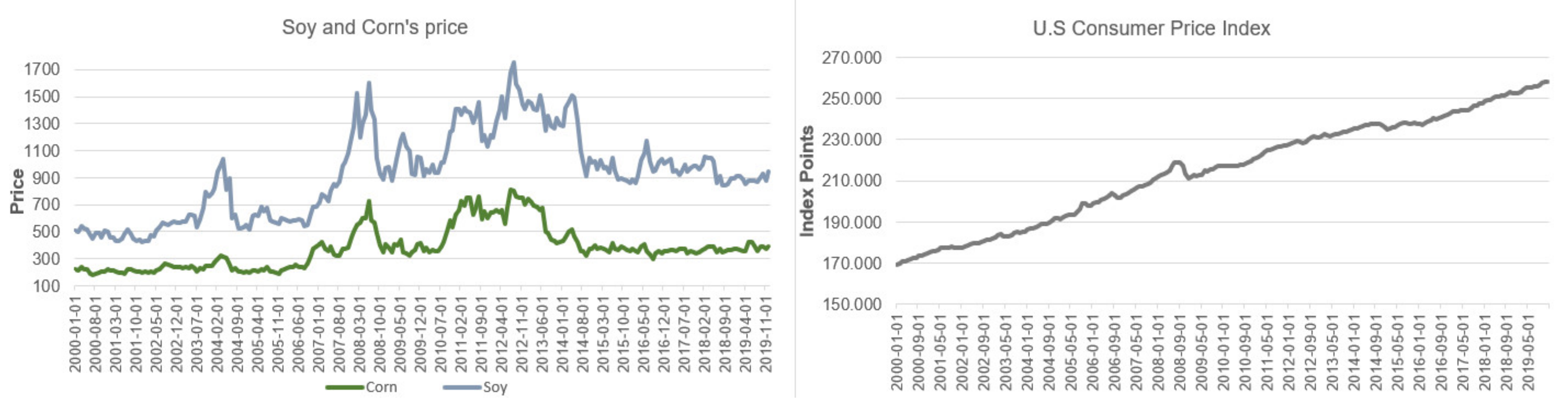
Soy Generalized Model

As already stated, an OLS with non-stationary variables would very likely generate spurious regression. All variables were found to be stationary at first difference (order of integration l (1)); therefore, the ordinary least squared regression was performed according to the following transformation.
1. OLS using variables in the first difference.
Without the pair of USD/BRL:
The regression on the level: Soy = β0 + β1 FxRate + β2 IntRate + ei
The regression on the first difference: Δ Soy = β0 + β1 Δ FxRate + β2 Δ IntRate + ei
Results of the generalized model excluding the variable USD/BRL for soy are presented in Table 1.
The result of this regression shows a significance at the 1% level for the regressor Fx. rate, and its coefficient shows that a change of one index unit in the dollar index would result in a decrease of USD 9.40 in the future market of soybeans. For the interest rate, the coefficient suggests that a unit decrease in this variable (in percent) would cause a decrease of USD 26.7 in the future soy markey; however, its p-value suggests no significance. The possible reasons for the insignificance of this variable will be discussed later.
We now add the variable USD/BRL, which is more relevant to soy as Brazil is the largest and most competitive producer of this agricultural commodity.
With the pair USD/BRL:
The regression on the level: soy = β0 + β1 FxRate + β2 IntRate + β3 USD/BRL + ei
The regression on the first difference: Δ soy = β0 + β1 Δ FxRate + β2 Δ IntRate + β3 Δ USD/BRL + ei
Results of the generalized model inclusive the variable USD/BRL for soy are presented in Table 2.
The results with the variable USD/BRL vary considerably. With the inclusion of interest rate, no changes occurred; however, with Fx. rate and the newly added variable, we can observe a significant influence. Fx. rate now shows significance at the 5% level (it is no longer 1%), showing that a change of one index unit in the dollar index would result in a fall of USD 7.04 dollars in the soy contract. The pair of U.S. dollar and Brazilian Real showed high significance, at the 0.1% level, with a coefficient suggesting that a unit change in the currency pair would result in a decrease of USD 142 in the contract for soy. Such a high result is obtained only for this commodity due to its close relation to the Brazilian economy; for corn and sugar, the impact is much lower, as will be displayed in future models. As the price formation of a commodity involves many variables, and the most relevant are the ones related to the production/exploration of the commodity, a model with purely monetary indicators would have low R² (without USD/BRL 0.03169, with USD/BRL 0.08732).
2. Engle–Granger Cointegration test
As the conversion of data to first differences causes a loss of information in the time series, further testing should be conducted to establish relations between the variables. To check for a possible long-term relation between variables, we will run the Engle–Granger test for cointegration. This cointegration test is suitable for two variables; therefore, three separate tests will be performed: soy/Fx. rate and soy/interest rate. A test with the four variables together will be executed accordingly.
(1a)
OLS: soy as the dependent variable and Fx. rate as the only independent variable.
(1b)
OLS: soy as the dependent variable and interest rate as the only independent variable.
(1c)
OLS: soy as the dependent variable and the pair USD/BRL as the only independent variable.
(2)
Residuals of the regression are stored to test for cointegration.
(3)
The test results are shown in Table 3.
Ho: There is no cointegration between soy prices and the other variable.
H1: There is cointegration between soy prices and the other variable.
[Rejection: |t| > 1.96]
The results, in absolute terms, are higher than t-statistic 1.96. Therefore, the null hypothesis can be rejected, and we can assume that cointegration between the variables exists for all “combinations”. This result indicates a possible long-term relation between soy prices and exchange rate, between soy prices and interest rates, and between soy prices and the pair USD/BRL.
3. The equation for OLS with non-stationary data + autocorrelation of data.
If a regression was conducted without checking for stationary, the resulting equation would be:
Soy = 2506.714 − 15.225FxRate − 81.938IntRate + ei
(2 × 10⁻¹⁶) *** (<2 × 10⁻¹⁶) *** (<2 × 10⁻¹⁶) ***
Soy = 2495.981 − 14.963 FxRate − 82.651IntRate − 5.013 USD/BRL + ei
(2 × 10⁻¹⁶)*** (5.94 × 10⁻¹⁴)*** (<2 × 10⁻¹⁶)*** (0.85)
With non-stationary data, USD/BRL would not affect the price of soy contracts—a conclusion that would not pertain in real life. Both non-stationary models have R-squared values of 0.6183.
Corn Generalized Model
1. OLS using variables in first difference.
Following the same method, two separate regressions will be tested.
Without the pair USD/BRL:
The regression on the level: corn = β0 + β1 FxRate + β2 IntRate + ei
The regression on the first difference: Δcorn = β0 + β1 Δ FxRate + β2 Δ IntRate + ei
Results of the generalized model excluding the variable USD/BRL for corn are presented in Table 4.
With similar results to soy’s first regression, for corn, Fx. rate is significant, but interest rate is not. Exchange rate is significant at the 5% level, and has milder impact on prices, as a change of one index unit in the dollar index would result in a decrease of USD 3.85 in corn future contract prices. Once again, interest rate has no influence on contract price, and its coefficient shows that a percentage change in interest rate would result in an increase of USD 1.86 in corn’s future contract prices.
After adding the currency pair to the regression, we see a very slight change.
With the pair USD/BRL:
The regression on the level: corn = β0 + β1 FxRate + β2 IntRate + β3 USD/BRL + ei
The regression on the first difference: Δcorn = β0 + β1 Δ FxRate + β2 Δ IntRate + β3 Δ USD/BRL + ei
Results of the generalized model inclusive the variable USD/BRL for corn are presented in Table 5.
Interest rate remains irrelevant to corn’s contract prices in this model, and with these variables. However, Fx. rate shows significance at the 10% level, with a very similar coefficient. The variable of the pair of U.S dollar and Brazilian Real has significance at the 10% level as well, and suggests that a unit change in the currency pair would result in a decrease of USD 35.9 in the corn contract price, which is less than that seen for soy, but is more than that for sugar. Chinese and U.S. trade policy variables in another model, such as one specific for corn, could express a more realistic relation regarding the price formation of this commodity. As stated for soy, a model with purely monetary indicators would have low R² (without USD/BRL, 0.03873; with USD/BRL, 0.03873).
2. Engle–Granger cointegration test
As done for soy:
(1a)
OLS: corn as the dependent variable and Fx. rate as the only independent variable.
(1b)
OLS: corn as the dependent variable and interest rate as the only independent variable.
(1c)
OLS: corn as the dependent variable and the pair USD/BRL as the only independent variable.
(2)
Residuals of the regression are stored to test for cointegration.
(3)
The test results are shown in Table 6.
Ho: There is no cointegration between corn prices and the other variable.
H1: There is cointegration between corn prices and the other variable.
[Rejection: |t| > 1.96]
The test provides evidence of a possible long-term relation between corn and each variable individually, as the null hypothesis can be rejected for all three t-statistic results. The Johansen cointegration test, which is a more sophisticated method, could be performed; however, it could not show whether the cointegration is related to the commodity specifically, and could reflect a cointegration of exchange rate and interest rate, or of USD/BRL and interest rate. This method can investigate the relations between the regressors and the commodities.
3. Equation for OLS with non-stationary data + autocorrelation of data.
This again shows the vastly different result derived from a regression with non-stationary time series.
Corn = 1147.1606 − 7.5869 FxRate − 29.6727 IntRate + ei
(<2 × 10⁻¹⁶) *** (<2 × 10⁻¹⁶) *** (2.83 × 10⁻¹³) ***
Corn = 1098.433 − 6.397 FxRate − 32.911 IntRate − 22.759 USD/BRL + ei
(<2 × 10⁻¹⁶) *** (2.86 × 10⁻⁹) *** (8.87 × 10⁻¹³) *** (0.122)
Sugar Generalized Model
Lastly, sugar has the special characteristic of being regressed with the pair USD/INR, which analyzes the influence of the second largest sugar producer in the world, and how it behaves in a regression with the largest producer (Brazil).
1. OLS using variables in first difference.
Without the pair USD/BRL:
The regression on the level: sugar = β0 + β1 FxRate + β2 IntRate + ei
The regression on the first difference: Δsugar = β0 + β1 Δ FxRate + β2 Δ IntRate + ei
Results of the generalized model excluding the variable USD/BRL for sugar are presented in Table 7.
Differently from previous regressions, both variables for sugar have no significance. In terms of the coefficient, a change of one index unit in the dollar index would result in a small decrease of USD 0.09 in the contract for sugar, and a percent change in the interest rate would implicate a reduction of USD 0.16 in the contract.
The regression with USD/BRL only shows significance for the newly added variable.
With the pair USD/BRL:
The regression on the level: sugar = β0 + β1 FxRate + β2 IntRate + β3 USD/BRL + ei
The regression on first difference: Δsugar = β0 + β1 Δ FxRate + β2 Δ IntRate + β3 Δ USD/BRL + ei
Results of the generalized model inclusive the variable USD/BRL for sugar are presented in Table 8.
Exchange rate and interest rate did not become significant in the new regression, and their coefficients were diminished. The added variable USD/BRL showed significance at the 5% level, and its coefficient indicates that a unit change in the pair would result in a decrease of USD 1.64 in sugar contract prices. Low rates of R² persist (without USD/BRL, 0.008437; with USD/BRL, 0.008437)
To visualize the influence of the Indian Rupee, the variable USD/INR is added to the model. The model outcome after adding USD/INR into the model is presented in Table 9.
Checking the influence of the Indian Rupee in the model:
Model 1 = with all variables; model 2 = without USD/BRL.
For the model with all variables, only USD/BRL was significant (at the 10% level), and its coefficient indicates that a unit change in the pair’s value would implicate a decrease of USD 1.29 in the sugar contract price. The Indian Rupee seems to be insignificant, as well did the other variables. However, when USD/BRL is removed from the model, USD/INR becomes significant at the 5% level, with a coefficient that indicates that a unit change in the pair’s value would implicate a decrease of USD 0.20 in the contract of sugar. As for the other two commodities, the R² is still low (with all variables, 0.039; without USD/BRL, 0.02765).
2. Engle–Granger cointegration test
(1a)
OLS: sugar as the dependent variable and Fx. rate as the only independent variable.
(1b)
OLS: sugar as the dependent variable and interest rate as the only independent variable.
(1c)
OLS: sugar as the dependent variable and the pair USD/BRL as the only independent variable.
(1d)
OLS: sugar as the dependent variable and the pair USD/INR as the only independent variable.
(2)
Residuals of the regression are stored to test for cointegration.
(3)
The test results are shown in Table 10.
Ho: There is no cointegration between sugar prices and the other variable.
H1: There is cointegration between sugar prices and the other variable.
[Rejection: |t| > 1.96]
The Engle–Granger cointegration test suggests that there is a long-term relationship between sugar and each other variable, as all four t-statistic values were higher than 1.96.
3. Equation for OLS with non-stationary data + autocorrelation of data.
If non-stationary time series were used, the regression results would be:
Sugar = 39.54598 − 0.24671 FxRate − 1.25464 IntRate + ei
(<2 × 10⁻¹⁶) *** (4.62 × 10⁻¹⁵) *** (2.28 × 10⁻¹³) ***
Sugar = 34.45248 − 0.12229FxRate − 1.59315 IntRate − 2.37898USD/BRL + ei
(<2 × 10⁻¹⁶)*** (0.00432)** (<2 × 10⁻¹⁶)*** (9.82 × 10⁻¹⁵)***
Sugar = 24.92721 − 0.17316FxRate − 0.90654IntRate − 5.35071 USD/BRL + 0.39226USD/INR + ei
(<2 × 10⁻¹⁶) *** (3.60 × 10⁻⁶) *** (1.62 × 10⁻⁷) *** (<2 × 10⁻¹⁶) *** (<2 × 10⁻¹⁶) ***

4.2. Model 2

Soy’s Expansionary Period Model
For all three commodities, the same six regressions will be executed to analyze the different responses of the regressors.
(1)
Soy = β0 + β1FxRate + ei
(2)
Soy = β0 + β1FxRate + β2 Consumer’s Loans + ei
(3)
Soy = β0 + β1FxRate + β2 Consumer’s Loans + β3Fx. Emerging Countries ei
(4)
Soy = β0 + β1FxRate + β2 Consumer’s Loans + β3Fx. Emerging Countries + β4ECB Assets + ei
(5)
Soy = β0 + β1 Consumer’s Loans + β2 Fx. Emerging Countries + ei
(6)
Soy = β0 + β1FxRate + β2Fx. Emerging Countries + ei
For soybeans, in every regression, one variable showed significance, but that was not the case for corn and sugar. For soy, the dollar index for emerging markets was significant in every regression in which it was included, while for the other two commodities, it was only significant once. Results for soyobtained from our expansionary model are dispayed in Table 11 and Table 12.
For the first two regressions, the Fx. rate showed significance at the 5% level, with a similar coefficient of approximately 13.9. In the third regression, with the inclusion of a dollar index for the emerging countries, this significance was lost, and the newly added variable became the only significant one, at the 5% level. Fx. emerging countries’ coefficient suggests that a change of an index unit would result in a decrease of USD 17.6 in the soy contract price. In the fourth regression, the ECB asset variable was added; however, due to the data format (first difference, to achieve stationarity), it disordered the regression and generated small coefficients. Nevertheless, Fx. emerging countries remained significant at the 5% level.
In the fifth regression, Fx. emerging countries achieved significance at the 1% level when regressed with only the consumer’s loan regressor for soy. It retained a reasonably constant coefficient for every regression. In the last regression, the Fx. rate showed no significance; however, when regressed solely with soy, it showed a 5% level significance. It is interesting to see how another dollar index (for emerging markets) has a greater impact on the dependent variable, and, when compared to the previous five regressions, the smallest coefficient for Fx. rate occurred when the other regressor was Fx. emerging countries.
Corn expansionary period model
(1)
Corn = β0 + β1FxRate + ei
(2)
Corn = β0 + β1FxRate + β2 Consumer’s Loans + ei
(3)
Corn = β0 + β1FxRate + β2 Consumer’s Loans + β3Fx. Emerging Countries ei
(4)
Corn = β0 + β1FxRate + β2 Consumer’s Loans + β3Fx. Emerging Countries + β4ECB Assets + ei
(5)
Corn = β0 + β1 Consumer’s Loans + β2 Fx. Emerging Countries + ei
(6)
Corn = β0 + β1FxRate + β2Fx. Emerging Countries + ei
This model for corn showed the lowest number of significant regressors, which was not the case for the “generalized model”, when sugar showed the lowest number. The result pertains in reality, as the United States is the largest corn producer, and the regressors try to capture some influence of the monetary expansion flowing from this country to other commodity producers (usually developing nations). Results for corn obtained from our expansionary model are dispayed in Table 13 and Table 14.
In the fifth regression, Fx. emerging countries becomes significant for the first and only time, at the 5% level, indicating that an index unit change in the dollar index would result in a decrease of USD 7.69 in the price of corn. When compared to the fifth regression for soy, this dollar index for emerging markets was significant at the 1% level, and implicated a USD 19.7 decrease in the commodity contract for each index unit change. In the last regression, both regressors showed no significance, and the coefficient for Fx. emerging countries was about one-quarter of the value of the same regression for soy.
Sugar expansionary period model
(1)
Corn = β0 + β1FxRate + ei
(2)
Sugar = β0 + β1FxRate + β2 Consumer’s Loans + ei
(3)
Sugar = β0 + β1FxRate + β2 Consumer’s Loans + β3Fx. Emerging Countries ei
(4)
Sugar = β0 + β1FxRate + β2 Consumer’s Loans + β3Fx. Emerging Countries + β4ECB Assets + ei
(5)
Sugar = β0 + β1 Consumer’s Loans + β2 Fx. Emerging Countries + ei
(6)
Sugar = β0 + β1FxRate + β2Fx. Emerging Countries + ei
A different result was derived when the variable consumer’s loan was added to sugar, which variable was not present for the previous two commodities. Due to the lower price of contracts for sugar, sugar’s coefficients (which express changes in contract prices) were also lower than soy and corn’s. For a brief comparison, the mean monthly price of sugar contracts for the period was USD 17.69, for corn it was USD 480.75, and for soy it was USD 1152.866. Results for sugar obtained from our expansionary model are dispayed in Table 15 and Table 16.
Showing the same development as the previous two commodities, when Fx. rate is regressed with sugar, it shows significance at the 5% level. In the second regression, this variable remained significant at the same level; however, differently from soy and corn, the variable consumer’s loan was significant at the 5% level, and it remained significant in the third regression, when the dollar index for emerging countries was added. In the third regression for soy, Fx. emerging countries was significant, but sugar was not in the third and fourth regressions. Only in the fifth regression did this variable become significant, along with the consumer’s loans variable, which appeared to be relevant in most cases. For the last regression, both Fx. rate and Fx. emerging countries showed no significant effect on the price of sugar contracts.
Results on responsiveness to monetary variables obtained from our model are summarized in Table 17.

5. Discussion

Corn’s price formation is the most complex of all three discussed commodities. It was shown to be the least responsive commodity, calling for a deeper discussion on the impact of liquidity on this asset. Differently from soy and sugar, corn is largely produced in the United States (half of the world’s production comes from there), and it is extensively subsidized by the government. Former President George W. Bush signed the Energy Policy Act of 2005, a federal law that, among other things, increased biofuel’s share in the gasoline sold in the United States. This law guarantees the demand for corn. Until 2011, corn was the most subsidized crop in the U.S. In the general model for corn, the only significant variable was the exchange rate, and in the expansionary model, the variable of emerging markets’ exchange rates was significant once. These two results are compliant with expectation pertaining to such a protected commodity. Global liquidity did not affect corn in a milder way. Corn prices experienced a sharp increase at rates that were the same as or higher than other commodities; however, a large portion of its price arrives from government subsidies, as well as trade and tax benefits, which could not be captured by the model. It is likely that if the variable “subsidy in dollars per bushel” was added, it would better explain the price behavior of corn, but not that of soy and sugar.
Regarding the massive outflow of dollars to emerging economies, the central question is: would the price of corn be responsive to this increase in demand in emerging markets in the same way that soy and sugar were? It seems that the used indicators could not capture that feature. The main point derived from the responsiveness of corn’s price is that, differently from the other two commodities, it is subject to a trade policy that makes foreign corn less competitive on the American market, but it also makes American corn less competitive to foreign markets. U.S. trade policy can be a barrier of entry to American producers in large emerging economies, especially the ones that also export commodities. The results for soy and sugar are different, because they can respond more freely to the indicators of our models.
We argue that the “risk-taking” spillover channel is appropriate for soy and sugar for the following reason: as the loan books of financial institutions become less risky, they have a higher capacity to lend (the core assumption of this channel). American farmers wishing to meet the high demand for corn on the world market would be willing to take the risk to borrow credit in order to engage in this commodity production; however, they are aware that the current large producers benefit from government subsidies, and are involved in sizable lobbying activities, so they will end up not engaging in corn production (choosing another crop).
Brazilian farmers would not face the same problem when producing soy or sugar; therefore, the risk-taking channel is capable of greater spillover effects for these three commodities in Brazil, Mexico, India, South Africa, Indonesia, etc. Lastly, we consider corn, and we disagree with Chalfant et al. [26], who argued that agricultural commodities would adapt to price changes more rapidly as they are less differentiated than non-agricultural commodities, especially in the short term. In real life, considering trade policies and economic–political blocks such as NAFTA, the European Union or Mercosur, short-term adaptations of price would certainly be prevented by the Central Banks’ instruments for political reasons or pressures from groups of interest.
The data for sugar give interesting results, as this commodity was the most responsive to the variable “loans to consumers”. This result is not surprising, as sugarcane is the highest-producing crop in the world, and has greater usability in the ordinary lives of consumers; sugar is present in virtually all food industries. Barsky and Killian [15] found that “price increases do not appear to be related to commodity-specific supply shocks, but are consistent with an economic boom fueled by monetary expansion”. A possible reason for this depends on the concept of portfolio rebalancing. Additionally, Neely [9] argued that private ownership of securities decreases when the Central Bank starts purchasing them under an expansionary policy (the authors discuss quantitative easing specifically), resulting in a portfolio rebalance. Once this rebalancing takes place, investors are willing to allocate their capital to international assets, and when they actually “export their dollars” to countries with better investment opportunities, the spillover happens. Abundant credit allied with a devalued dollar (during commodities’ boom) increases mass consumption, and sugar seems to be more sensitive to mass consumption when compared to soy and corn.
Another discussion topic for sugar derives from the generalized model, which states that Brazil is the largest sugarcane producer and India is the second largest one. However, the significance for India’s currency is higher than that for the Brazilian one. A plausible explanation could be the share of sugarcane in both countries’ GDPs—the share in India is slightly higher than in Brazil; therefore, we can expect that policy signaling, large-scale asset purchases, portfolio rebalancing, or any other minetary instrument applied to the Indian Rupee will have a stronger effect on India’s sugar sector than on Brazil’s. Scrimgeour [17] states that responsiveness to unexpected monetary policy actions is heterogeneous to individual commodities, and these responses are correlated with the volume of the product. Our results show that the volume in India is greater (in proportion to the national output), so the greater significance of the Rupee than of the Real can be expected. The last interesting result for sugar also relates to the Scrimgeour’s study. He stated that for each percentage point reduction in interest rates (by the FED), there is an increase in commodity prices by roughly 5%. In the generalized model for sugar, including both USD/BRL and USD/INR, the coefficient of the interest rate was roughly −4%, which is almost inversely proportional to the result of his study: for each percentage point increase in interest rate, sugar prices decrease by 4%.
Soy seems to give the most predictable results in both models, making clear the importance of Brazil’s exchange rate and the variable “Fx. emerging countries” to the commodity’s price formation. The uniqueness of soy is that it does not have as widespread cultivation as sugarcane and corn. In the 1960’s, Brazil started growing soy as an alternative to wheat during summer, after research into adapting this crop to tropical weather. As such, many countries face a technical barrier to becoming a top-tier competitor in the soy market, and from that, we derive Brazil’s relevance. Differently from sugar, soy was not responsive to loans to consumers. Our interpretation of such a result depends on the usability of soy. Sugar is used in the whole of the food industry, but soy is largely used to feed livestock. Bordo [19] proposed a pattern of commodity price adaptation to monetary changes, determined by different contract lengths. As future contracts for soy are largely purchased by farmers and entrepreneurs in the livestock industry, the contracts here tend to be longer than for sugar. Bordo [19] maintains that longer contracts make commodities less flexible to monetary changes, and the variable “loans to consumers” captures the point at which the newly created liquidity reaches people’s bank accounts; that is significant for sugar, but not for soy. So why would foreign exchange rates would affect soy if it is less flexible? Because they affect contract terms, (1) they make it more/less advantageous for Brazilian farmers to export, and they (2) influence the decisions of contract owners to hold contracts until maturity or to sell them before maturity. Therefore, the only variables that showed significance for soy were related to exchange rates.

6. Conclusions

This study confirmed the preconceived and established idea that monetary policy and spillovers are able to affect agricultural commodities’ prices; however, the notion that each commodity responds in different ways to different variables is a key point. The main message of this paper is that commodities differ in their level of “sensibility” to different channels of liquidity. This paper offers an answer to the question regarding how expansionary monetary policy influences agricultural commodities’ prices, but also raises the question of which type of liquidity channel explains agricultural commodities’ prices better. Future research on specific channels could be performed to create a model that explains past prices and can forecast future ones.
Our findings confirm the intuition that global liquidity spills over from developed to developing economies, and impacts agricultural commodities’ prices. We argue that agricultural commodities should not be regarded as general categories, but individually. A separate look at coffee, coconut, sugar, oilseeds, corn, wheat, sunflower seeds, soy, rice, etc., is needed. It is not about the question, “can monetary policy affect agricultural commodities?” but instead “how can monetary policy affect the prices of future corn contracts?”
In particular, our results show that corn prices do not respond to the monetary indicators we tested, soy prices act as a proxy for the exchange rates of their producing countries, and sugar is highly sensible to people’s consumption.
In the case of soy, there seems to be a technology barrier facing most developing countries, and longer contracts make this commodity more sensitive to exchange rates than to large-scale asset purchases or putting credit for consumption in people’s hands. The following question is interesting, and poses a question for future research: if Brazil adopted protectionist measures for soy at the same rate as the U.S adopted them for corn, would exchange rates lose significance? The same question can be posed for sugar in India.
The conclusion for corn depends on the fact that it is a commodity with a certain resistance to the monetary indicators tested. A possible further research direction for corn could address the search for a monetary variable that better explains or predicts corn prices.
Consistently with the theoretical assumptions, the variable loans to consumers was significant for sugar, through increased consumption and investments of households. Our data confirm that an increase in loans to consumers, along with other monetary policies, would affect future sugar contracts prices, but would not affect the futures of soy and corn.
The analysis presented in this paper offers an interesting lesson to those involved in trading with agricultural commodities, be they producers, intermediaries or buyers. We argue that, besides the indicators inherent to the production of the commodity, it is advisable to take into account the stage of the monetary cycle and monetary aggregates when considering the length of the future contract. As an example, if traders and producers that do not grow sugarcane understand that the economy is entering a period of expansionary monetary policies, they can adjust their portfolio to include assets related to sugar. Our models offer an insight into the differences in the sensitivity of some agricultural commodities to monetary indicators.

Author Contributions

Conceptualization, K.Č. and E.A.H.F.; methodology, K.Č. and E.A.H.F.; software, E.A.H.F.; validation, E.A.H.F. and K.Č.; formal analysis, E.A.H.F.; investigation, E.A.H.F. and K.Č.; resources, K.Č. and E.A.H.F.; data curation, E.A.H.F.; writing—original draft preparation, E.A.H.F. and K.Č.; visualization, E.A.H.F. and K.Č.; writing, review and editing, K.Č.; supervision, K.Č.; project administration, K.Č.; funding acquisition, K.Č. All authors have read and agreed to the published version of the manuscript.

Funding

This research was funded by Prague University of Economics and Business, grant number VŠE IGS F5/2/2020.

Data Availability Statement

Data supporting reported results are available using the links below:

Conflicts of Interest

The authors declare no conflict of interest.

References

  1. UNCTAD—United Nations Conference on Trade and Development. Facts and Figures on Commodities and Commodities Trade. Geneva, Switzerland. 2013. Available online: https://unctad.org/press-material/facts-and-figures-commodities-and-commodities-trade (accessed on 11 April 2021).
  2. Bank for International Settlements (BIS). Global Liquidity—Concept, Measurement and Policy Implications. CGFS Papers, Bank for International Settlements, No. 45. 2011, pp. 4–5. Available online: https://www.bis.org/publ/cgfs45.pdf (accessed on 15 August 2021).
  3. Bahaj, S.; Reis, R. Central Bank Swap Lines; CESifo Working Paper, No.7124; Center for Economic Studies and ifo Institute (CESifo), University of Munich: Munich, Germany, 2018; p. 6. [Google Scholar]
  4. Landau, J.P. Global Liquidity: Public and Private. In Proceedings—Economic Policy Symposium; Hole, J., Ed.; Federal Reserve Bank of Kansas City: Kansas City, MO, USA, 2013; pp. 223–259. [Google Scholar]
  5. Mundell, R.A. Capital Mobility and Stabilization Policy under Fixed and Flexible Exchange Rates. Can. J. Econ. Political Sci./Rev. Can. d’Economique Sci. Polit. 1963, 29, 475–485. [Google Scholar] [CrossRef]
  6. Fleming, J.M. Domestic Financial Policies Under Fixed and under Floating Exchange Rates Politiques. Staff. Pap. -Int. Monet. Fund 1962, 9, 369–380. [Google Scholar] [CrossRef]
  7. Dornbusch, R. Expectations and exchange rate dynamics. J. Political Econ. 1976, 84, 1161–1176. [Google Scholar] [CrossRef]
  8. Joyce, M.; Lasaosa, A.; Stevens, I.; Tong, M. The Financial Market Impact of Quantitative Easing in the United Kingdom. Int. J. Cent. Bank. 2011, 7, 113–161. [Google Scholar]
  9. Neely, C.J. Unconventional Monetary Policy Had Large International Effects. J. Bank. Financ. 2015, 52, 101–111. [Google Scholar] [CrossRef]
  10. Hausman, J.; Wongswan, J. Global Asset Prices and FOMC Announcements. J. Int. Money Financ. 2011, 30, 547–571. [Google Scholar] [CrossRef]
  11. Tran, T.B.N.; Pham, H.C.H. The Spillover Effects of the US Unconventional Monetary Policy: New Evidence from Asian Developing Countries. J. Risk Financ. Manag. 2020, 13, 165. [Google Scholar] [CrossRef]
  12. Glick, R.; Leduc, S. Central Bank Announcements of Asset Purchases and the Impact on Global Financial and Commodity Markets. J. Int. Money Financ. 2012, 31, 2078–2101. [Google Scholar] [CrossRef]
  13. Bruno, V.; Shin, H.S. Capital Flows and the Risk-Taking Channel of Monetary Policy. J. Monet. Econ. 2015, 71, 119–132. [Google Scholar] [CrossRef]
  14. Huh, C.G.; Wu, J. Linkage between US monetary policy and emerging economies: The case of Korea’s financial market and monetary policy. Int. J. Econ. Sci. 2015, 4, 1–18, 1020472/ES201543001. [Google Scholar] [CrossRef] [Green Version]
  15. Barsky, R.; Kilian, L. Do We Really Know that Oil Caused the Great Stagnation? A Monetary Alternative. Natl. Bur. Econ. Res. Macroecon. Annu. 2001, 16, 137–183. [Google Scholar]
  16. Just, M.; Łuczak, A.; Kozera, A. Conditional Dependence Structure in the Precious Metals Futures Market. Int. J. Econ. Sci. 2019, 8, 81–93. [Google Scholar] [CrossRef]
  17. Scrimgeour, D. Commodity Price Responses to Monetary Policy Surprises. Am. J. Agric. Econ. 2015, 97, 88–102. [Google Scholar] [CrossRef] [Green Version]
  18. Anzuini, A.; Lombardi, M.J.; Pagano, P. The Impact of Monetary Policy Shocks on Commodity Prices. Int. J. Cent. Bank. 2013, 9, 125–150. [Google Scholar] [CrossRef] [Green Version]
  19. Bordo, M.D. Effects of Monetary Change on Relative Commodity Prices and the Role of Long Term Contracts. J. Political Econ. 1980, 88, 1088–1109. [Google Scholar] [CrossRef]
  20. Kyrtsou, C.; Labys, W. Evidence for chaotic dependence between US inflation and commodity prices. J. Macroecon. 2006, 28, 256–266. [Google Scholar] [CrossRef]
  21. Siami-Namini, S. Volatility Transmission among Oil Price, Exchange Rate and Agricultural Commodities Prices. Appl. Econ. Financ. 2019, 6, 41. [Google Scholar] [CrossRef]
  22. Frank, J.; Garcia, P. How Strong are the Linkages among Agricultural, Oil, and Exchange Rate Markets? In Proceedings of the NCCC-134 Conference on Applied Commodity Price Analysis, Forecasting, and Market Risk Management, St Louis, MO, USA, 19–20 April 2010. [Google Scholar]
  23. Musunuru, N. Causal Relationships between Grain, Meat Prices and Exchange Rates. Int. J. Food Agric. Econ. 2017, 5, 1–10. [Google Scholar]
  24. Belke, A.; Bordon, I.G.; Hendricks, T.W. Global liquidity and commodity prices—A cointegrated VAR approach for OECD countries. Appl. Financ. Econ. 2010, 20, 227–242. [Google Scholar] [CrossRef] [Green Version]
  25. Chen, J.; Griffoli, T.M.; Sahay, R. Spillovers from United States Monetary Policy on Emerging Markets: Different This Time? International Monetary Fund Working Paper No. 14/240; International netary Fund: Washington, DC, USA, 2014. [Google Scholar]
  26. Chalfant, J.A.; Love, H.A.; Rausser, G.C.; Stamoulis, K.G. The Effects of Monetary Policy on U.S. Agriculture; Working Paper No.409; University of California-Berkeley: Berkeley, CA, USA, 1986. [Google Scholar]
Figure 1. Transmission channels of quantitative easing [8].
Sustainability 13 09317 g001
Figure 2. Soy and corn prices and U.S. CPI. Data source: Chicago Mercantile Exchange and FED.
Sustainability 13 09317 g002
Figure 3. U.S. interest rate, highlighted period: January 2007–December 2016. Source: Federal Reserve Bank of St. Louis.
Sustainability 13 09317 g003
Table 1. Soy’s generalized del without USD/BRL.
VariableEstimatePr (>|t|)
(Intercept)1.7280.74172
Fx. Rate−9.3910.00733 **
Interest Rate−26.7080.39913
Resultant equation: soy = 1.728 − 9.391 FxRate − 26.708 IntRate + ei. (0.74172) (0.00733) ** (0.39913).
Table 2. Soy’s generalized model with USD/BRL.
VariableEstimatePr (>|t|)
(Intercept)2.7270.593551
Fx. Rate−7.0420.041441 *
Interest Rate−26.7080.180656
USD/BRL−142.0310.000195 ***
Soy = 2.727 − 7.042FxRate − 26.708 IntRate − 142.031USD/BRL + ei. (0.593551) (0.041441) * (0.180656) (0.000195) ***.
Table 3. Soy’s cointegration test.
(a) Soy Price~Fx Rate(b) Soy Price~Interest Rate(c) Soy Price~USD/BRL
Test statistic:−10.4191−10.0971−10.357
Table 4. Corn’s generalized model without USD/BRL.
Variable.EstimatePr (>|t|)
(Intercept)0.87260.7266
Fx. Rate−3.85110.0206 *
Interest Rate1.86140.9016
Corn = 0.8726 – 3.8511 FxRate + 1.8614IntRate + ei. (0.7266) (0.0206) * (0.9016).
Table 5. Corn’s generalized model with USD/BRL.
VariableEstimatePr (>|t|)
(Intercept)1.1250.6506
Fx. Rate−3.2570.0522
Interest Rate−1.9140.8991
USD/BRL−35.9060.0502
Corn = 1.125 − 3.257FxRate − 1.914 IntRate − 35.906 USD/BRL + ei. (0.6506) (0.0522). (0.8991) (0.0502).
Table 6. Corn’s cointegration test.
(a) Corn Price~Fx Rate(b) Corn Price~Interest Rate(c) Corn Price~USD/BRL
Test statistic:−10.5956−10.3639−10.5024
Table 7. Sugar’s generalized model without USD/BRL.
VariableEstimatePr (>|t|)
(Intercept)0.039630.700
Fx. Rate−0.092920.174
Interest Rate0.169730.784
Sugar = 0.03963 − 0.09292FxRate + 0.16973 IntRate + ei. (0.700) (0.174) (0.784).
Table 8. Sugar’s generalized model with USD/BRL.
VariableEstimatePr (>|t|)
(Intercept)0.0511710.6165
Fx. Rate−0.0657750.3391
Interest Rate−0.0028660.9963
USD/BRL−1.6413330.0297 *
Sugar = 0.051171 − 0.065775FxRate − 0.002866 IntRate − 1.641333USD/BRL + ei. (0.6165) (0.3391) (0.9963) (0.0297) *.
Table 9. Sugar’s generalized model with USD/BRL and USD/INR.
del(1)(2)
VariableEstimatePr (>|t|)EstimatePr (>|t|)
(Intercept)0.064810.52590.060280.5565
Fx. Rate−0.039730.5725−0.052090.4585
Interest Rate−0.036590.95290.079430.8976
USD/BRL−1.293140.0978
USD/INR−0.15860.1067−0.203590.0322
Table 10. Sugar’s cointegration test.
(a) Sugar Price~Fx Rate(b) Sugar Price~Interest Rate(c) Sugar Price~USD/BRL(d) Sugar Price~USD/INR
Test statistic:−12.1129−11.9406−12.0068−11.8438
Table 11. Soy’s expansionary model.
Scheme 1.(1)(2)(3)
VariableEstimatePr(>|t|)EstimatePr(>|t|)EstimatePr(>|t|)
Intercept4.5840.62274.172920.66136.409280.4977
Fx. Rate−13.8760.0265−13.939360.0266−3.138340.6948
Consumer’s loan 0.081380.81830.035290.9196
Fx. Emerging Countries −17.619130.0372
ECB Assets
Reg’s p-value0.02647 0.08389 0.02541
0.04139 0.04183 0.07747
R²- Adj0.0332 0.02531 0.0534
Table 12. Soy’s expansionary model (part II).
Regression(4)(5)(6)
VariableEstimatePr(>|t|)EstimatePr(>|t|)EstimatePr(>|t|)
Intercept4.340.64916.411340.4966.5940.4752
Fx. Rate−4.060.6119 −3.0780.6983
Consumer’s loan−0.010.96630.025090.9424
Fx. Emerging Countries−20.380.0192−19.73130.0025−17.6720.0355
ECB Assets1.44 × 10−40.1823
Reg’s p-value0.02575 0.009359 0.009359
0.09181 0.07738 0.07738
R²-Adj0.05995 0.06148 0.06148
Table 13. Corn’s expansionary model.
Corn Regression(1)(2)(3)
VariableEstimatePr(>|t|)EstimatePr(>|t|)EstimatePr(>|t|)
Intercept0.68380.88380.84970.8591.48150.758
Fx. Rate−7.11930.0235−7.09370.0247−4.042370.322
Consumer’s loan −0.03280.8537−0.045820.797
Fx. Emerging Countries −4.977450.244
ECB Assets
Reg’s p-value0.02348 0.07635 0.0901
0.0431 0.04338 0.05463
R²- Adj0.03492 0.02689 0.02997
Table 14. Corn’s expansionary model (part II).
Regression(4)(5)(6)
VariableEstimatePr(>|t|)EstimatePr(>|t|)EstimatePr(>|t|)
Intercept1.110.8211.484150.75751.2420.791
Fx. Rate−4.210.306 −4.120.309
Consumer’s loan−0.050.76−0.058950.7398
Fx. Emerging Countries−5.480.215−7.698060.01994.9090.248
ECB Assets2.62 × 10−50.636
Reg’s p-value0.1534 0.06323 0.03975
0.0565 0.04649 0.05409
R²- Adj0.02339 0.03005 0.03778
Table 15. Sugar’s expansionary model.
Sugar Regression(1)(2)(3)
VariableEstimatePr(>|t|)EstimatePr(>|t|)EstimatePr(>|t|)
Intercept0.11410.53420.1861810.31310.2095620.259
Fx. Rate−0.24930.0426−0.2381310.0496−0.1252050.4251
Consumer’s loan −0.0142490.0393−0.0147310.0334
Fx. Emerging Countries −0.184210.2634
ECB Assets
Reg’s p-value0.04262 0.01531 0.02246
0.03467 0.06952 0.07963
R²- Adj0.02642 0.05348 0.05562
Table 16. Sugar’s expansionary model (part II).
Regression(4)(5)(6)
VariableEstimatePr(>|t|)EstimatePr(>|t|)EstimatePr(>|t|)
Intercept0.180.3460.2096450.2580.13250.473
Fx. Rate−0.140.375 −0.15020.345
Consumer’s loan−0.020.026−0.0151380.0282
Fx. Emerging Countries−0.230.18−0.2684760.0344−0.16210.331
ECB Assets0.000.287
Reg’s p-value0.03029 0.01121 0.08042
0.08877 0.0745 0.04253
R²- Adj0.0568 0.05855 0.02602
Table 17. Summarized results.
Variables/CommodityGeneral delExpansionary del
Fx. RateInterest RateUSD/BRLFx. RateConsumer’s loanFx. Emerging CountriesECB Assets
CornMildly sensible- Mildly sensible---
Soy--Very sensible--Very sensible-
Sugar-- -Very sensible--
Publisher’s Note: MDPI stays neutral with regard to jurisdictional claims in published maps and institutional affiliations.

