
Built Environment Factors Influencing Prevalence of Hypertension at Community Level in China: The Case of Wuhan


Abstract
:1. Introduction
2. Study Area
3. Materials and Methods
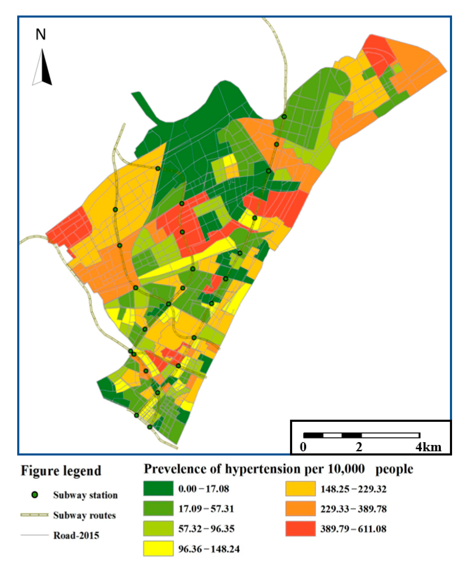
3.1. Collecting Hypertension Data for Visualized Images at Community Level
3.2. Calculation of Built Environment Indicators
3.2.1. Land Use
- Land use mix (LUM):
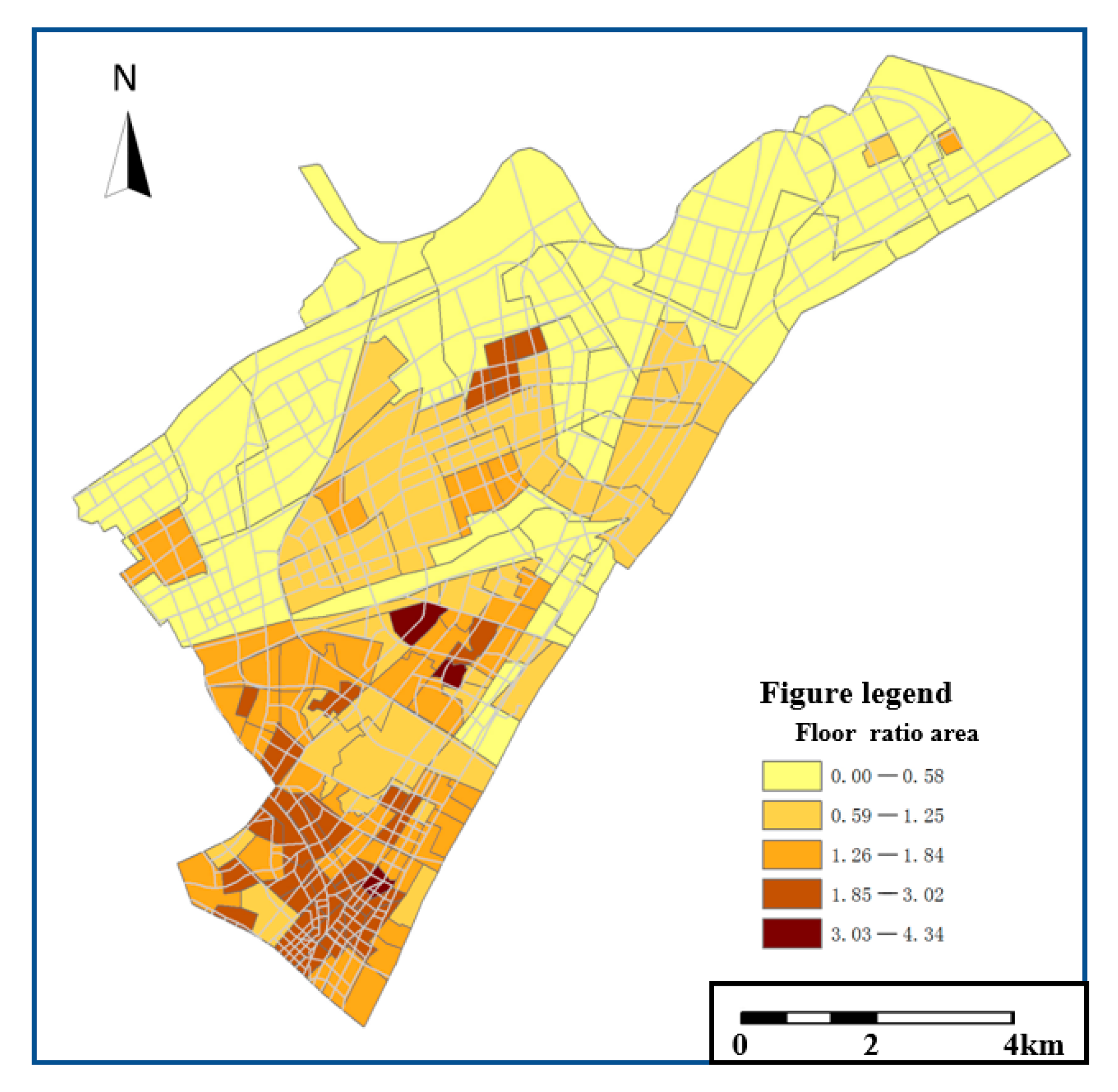
- Floor area ratio (FAR):
3.2.2. Transport
- Density of road networks:
- Destination accessibility:
- Public transport accessibility:
- Accessibility of public facilities:
3.2.3. Green Space
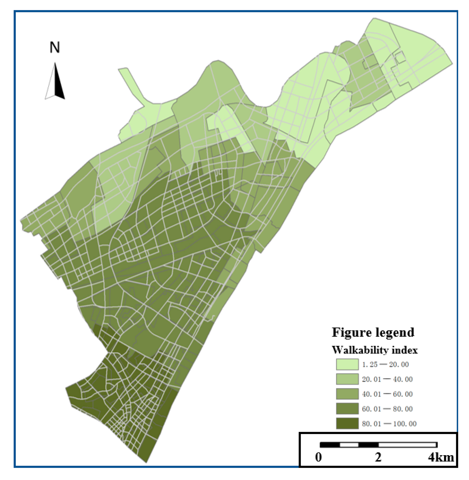
3.2.4. Urban Design
3.2.5. Income
3.3. Evaluating the Influences of Built Environment Indicators on the Prevalence of Hypertension
3.3.1. Multivariate Regression Model
3.3.2. Spatial Analysis Based on SLM and SEM
4. Results
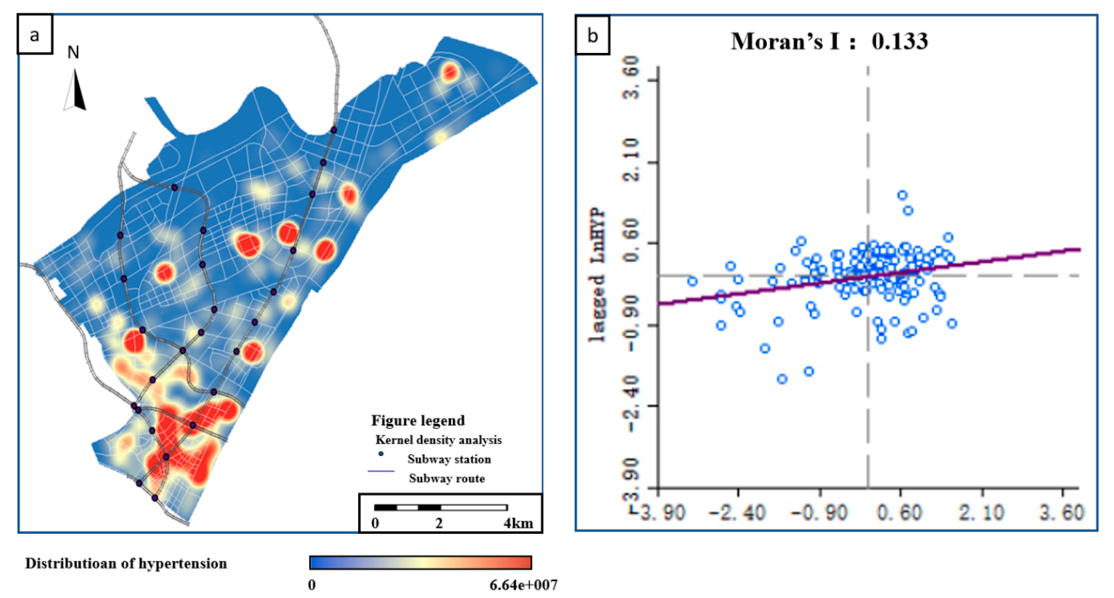
4.1. Spatial Clustering of the Hypertension Prevalence
4.2. Results of Multivariate Regression Models
4.3. The Performance of SEM and SLM
5. Discussion
5.1. The Significance of Influences of Built Environment Variables on Hypertension
5.2. Built Environment Factors that Affect the Prevalence of Hypertension Significantly
5.3. Other Built Environment Factors That Did Not Pass Significance Test
6. Conclusions
Author Contributions
Funding
Data Availability Statement
Acknowledgments
Conflicts of Interest
References
- Omran, A.R. The Epidemiologic Transition: A Theory of the Epidemiology of Population Change. Milbank Q. 2005, 83, 731–757. [Google Scholar] [CrossRef] [PubMed] [Green Version]
- Goenka, S.; Andersen, L.B. Urban design and transport to promote healthy lives. Lancet 2016, 388, 2851–2853. [Google Scholar] [CrossRef]
- Barrett, M.A.; Miller, D.; Frumkin, H. Parks and Health: Aligning Incentives to Create Innovations in Chronic Disease Prevention. Prev. Chronic Dis. 2014, 11, 63. [Google Scholar] [CrossRef] [PubMed] [Green Version]
- Webster, C. Refutation and the Scientific Knowledge Base of Urban Planning Practice. Urban Plan. Forum 2013, 3, 36–42. [Google Scholar]
- Wang, L.; Jiang, X.J. A Review of Research and Practice hotspot in healthy cities 2019. Sci. Technol. Guide 2020, 38, 164. [Google Scholar] [CrossRef]
- Sun, B.D.; Yin, C. Impact of built environment on residents’ health: Evidence from residents living in relocation housing. Urban and Reg. Plan. Res. 2018, 10, 48–58. [Google Scholar]
- Melanie, L.; Paula, H.; Helen, J.; Kathryn, B.; Iain, B.; Billie, G. Evidence-Informed Planning for Healthy Liveable Cities: How Can Policy Frameworks Be Used to Strengthen Research Translation? Curr. Environ. Health Rep. 2019, 6, 127–136. [Google Scholar]
- Garfinkel-Castro, A.; Kim, K.; Hamidi, S.; Ewing, R. Obesity and the built environment at different urban scales: Examining the literature. Nutr. Rev. 2017, 75, 51–61. [Google Scholar] [CrossRef] [PubMed]
- Lalonde, M. A New Perspective on the Health of Canadians: A Working Document; Government of Canada: Ottawa, ON, Canada, 1974; pp. 1–76. [Google Scholar]
- Handy, S.L.; Boarnet, M.G.; Ewing, R.E.; Killingsworth, R.E. How the built environment affects physical activityy: Views from urban planning. Am. J. Rev. Med. 2002, 23, 64–73. [Google Scholar]
- Papas, M.A.; Alberg, A.J.; Ewing, R.; Helzlsouer, K.J.; Gary-Webb, T.; Klassen, A.C. The Built Environment and Obesity. Epidemiologic Rev. 2007, 29, 129–143. [Google Scholar] [CrossRef] [Green Version]
- Mytton, O.T.; Nick, T.; Harry, R.; Charlie, F. Green space and physical activity: An observational study using Health Survey for England data. Health Place 2012, 18, 1034–1041. [Google Scholar] [CrossRef] [Green Version]
- Sallis, J.F.; Cerin, E.; Kerr, J.; Adams, M.A.; Sugiyama, T.; Christiansen, L.B.; Schipperijn, J.; Davey, R.; Salvo, D.; Frank, L.D.; et al. Built environment, physical activity, and obesity: Findings from the international physical activity and environment network (IPEN) adult study. Annu. Rev. Public Health 2020, 41, 119–139. [Google Scholar] [CrossRef] [Green Version]
- Höijer, K.; Lindö, C.; Mustafa, A.; Nyberg, M.; Olsson, V.; Rothenberg, E.; Sepp, H.; Wendin, K. Health and Sustainability in Public Meals—An Explorative Review. Int. J. Environ. Res. Public Health 2020, 17, 621. [Google Scholar] [CrossRef] [Green Version]
- Collado, S.; Staats, H.; Corraliza, J.A.; Hartig, T. Restorative Environments and Health. In Handbook of Environmental Psychology and Quality of Life Research; Fleury-Bahi, G., Pol, E., Navarro, O., Eds.; Springer International Publishing AG: Cham, Switzerlands, 2016; pp. 127–148. [Google Scholar]
- Grant, M.; Braubach, M. Evidence review on the spatial determinants of health in urban settings. In Urban Planning, Environment and Health: From Evidence to Policy Action. Meeting Report. Annex 2; WHO Regional Office for Europe: Copenhagen, Denmark, 2010; pp. 22–97. [Google Scholar]
- Nieuwenhuijsen, M.; Khreis, H. Integrating Human Health into the Urban Development and Transport Planning Agenda: A Summary and Final Conclusions. In Integrating Human Health into Urban and Transport Planning: A Framework; Nieuwenhuijsen, M., Khreis, H., Eds.; Springer International Publishing AG: Cham, Switzerland, 2019; pp. 707–718. [Google Scholar]
- Malambo, P.; Kengne, A.P.; De Villiers, A.; Lambert, E.V.; Puoane, T. Built environment, selected risk factors and major cardiovascular disease outcomes: A systematic review. PLoS ONE 2016, 11, e0166846. [Google Scholar] [CrossRef]
- Malambo, P.; Kengne, A.P.; Lambert, E.V.; Villers, A.D.; Puoane, T. Association between perceived built environment and prevalent hypertension among South African adults. Adv. Epidemiol. 2016, 2016, 1–11. [Google Scholar] [CrossRef] [Green Version]
- Sarkar, C.; Webster, C.; Gallacher, J. Association between adiposity outcomes and residential density: A full-data, cross-sectional analysis of 419 562 UK Biobank adult participants. Lancet Planet. Health 2017, 1, e277–e288. [Google Scholar] [CrossRef] [Green Version]
- Andreucci, M.B.; Russo, A.; Olszewska-Guizzo, A. Designing Urban Green Blue Infrastructure for Mental Health and Elderly Wellbeing. Sustainability 2019, 11, 6425. [Google Scholar] [CrossRef] [Green Version]
- Olszewska-Guizzo, A.; Sia, A.; Fogel, A.; Ho, R. Can exposure to certain urban green spaces trigger frontal alpha asymmetry in the brain?—Preliminary findings from a passive task EEG study. Int. J. Environ. Res. Public Health 2020, 17, 394. [Google Scholar] [CrossRef] [Green Version]
- Beute, F.; Andreucci, M.B.; Lammel, A.; Davies, Z.; Glanville, J.; Keune, H.; Marselle, M.; O’Brien, L.A.; Olszewska-Guizzo, A.; Remmen, R.; et al. Types and Characteristics of Urban and Peri-Urban Green Spaces Having an Impact on Human Mental Health and Wellbeing. An EKLIPSE Expert Working Group Report; UK Centre for Ecology & Hydrology: Wallingford, UK, 2020. [Google Scholar]
- Grant, M.; Brown, C.; Caiaffa, W.T.; Capon, A.; Corburn, J.; Coutts, C.; Crespo, C.J.; Ellis, G.; Ferguson, G.; Fudge, C.; et al. Cities and health: An evolving global conversation. Cities Health 2017, 1, 1–9. [Google Scholar] [CrossRef]
- Rao, M.; Prasad, S.; Adshead, F.; Tissera, H. The built environment and health. Lancet 2007, 370, 1111–1113. [Google Scholar] [CrossRef]
- Krieger, N.; Chen, J.T.; Waterman, P.D.; Soobader, M.-J.; Subramanian, S.V.; Carson, R. Choosing area based socioeconomic measures to monitor social inequalities in low birth weight and childhood lead poisoning: The Public Health Disparities Geocoding Project (US). J. Epidemiol. Community Health 2003, 57, 186–199. [Google Scholar] [CrossRef] [PubMed] [Green Version]
- Ewing, R.; Meakins, G.; Hamidi, S.; Nelson, A.C. Relationship between urban sprawl and physical activity, obesity, and morbidity – Update and refinement. Health Place 2014, 26, 118–126. [Google Scholar] [CrossRef] [Green Version]
- Auchincloss, A.H.; Roux, A.V.D. A new tool for epidemiology: The usefulness of dynamic-agent models in understanding place effects on health. Am. J. Epidemiol. 2008, 168, 1–8. [Google Scholar] [CrossRef] [Green Version]
- Galea, S.; Riddle, M.; Kaplan, G.A. Causal thinking and complex system approaches in epidemiology. Int. J. Epidemiol. 2010, 39, 97–106. [Google Scholar] [CrossRef]
- Pinto, A.; McGaw-Césaire, J.; Petrokofsky, C. Spatial Planning for Health: An Evidence Resource for Planning and Designing Healthier Places; Public Health England: London, UK, 2017. [Google Scholar]
- Sugiyama, T.; Koohsari, M.J.; Mavoa, S.; Owen, N. Activity-Friendly Built Environment Attributes and Adult Adiposity. Curr. Obes. Rep. 2014, 3, 183–198. [Google Scholar] [CrossRef] [PubMed]
- Albanese, N.N.; Friedberg, J.P.; Rundle, A.; Quinn, J.; Neckerman, K.; Lipsitz, S.R.; Natarajan, S. Association of the built environment and neighborhood resources with obesity-related health behavior (Abstracts from the 38th Annual Meeting of the Society of General Internal Medicine). J. Gen. Intern. Med. 2015, 30, 45–551. [Google Scholar]
- Frank, L.D.; Andresen, M.A.; Schmid, T.L. Obesity relationships with community design, physical activity, and time spent in cars. Am. J. Prev. Med. 2004, 27, 87–96. [Google Scholar] [CrossRef]
- Liu, Z.; Yang, D. Exploring the impact of the built environment on outdoor recreational activities of the elderly in the neighborhood: A comparative study of four typical neighborhood in Dalian. J. Archit. 2016, 6, 25–29. [Google Scholar]
- Cerin, E.; Leslie, E.; Du Toit, L.; Owen, N.; Frank, L.D. Destinations that matter: Associations with walking for transport. Health Place 2007, 13, 713–724. [Google Scholar] [CrossRef]
- Forsyth, A.; Hearst, M.; Oakes, J.M.; Schmitz, K.H. Design and Destinations: Factors Influencing Walking and Total Physical Activity. Urban Stud. 2008, 45, 1973–1996. [Google Scholar] [CrossRef]
- Ewing, R.; Cervero, R. Travel and the Built Environment: A Meta-Analysis. J. Am. Plan. Assoc. 2010, 76, 265–294. [Google Scholar] [CrossRef]
- Jiang, B.; Zhang, T.; Sullivan, W.C. Healthy cities: Mechanisms and research questions regarding the impacts of urban green landscapes on public health and well-being. Landsc. Archit. Front. 2015, 3, 24–35. [Google Scholar]
- Ulrich, R.S. View through a window may influence recovery from surgery. Science 1984, 224, 420–421. [Google Scholar] [CrossRef] [PubMed] [Green Version]
- China Cardiovascular Disease Report 2018; National Center for Cardiovascular Disease; China Encyclopedia Press: Beijing, China, 2019.
- Wang, Z.; Chen, Z.; Zhang, L.; Wang, X.; Hao, G.; Zhang, Z.; Shao, L.; Tian, Y.; Dong, Y.; Zheng, C.; et al. Status of Hypertension in China. Circulation 2018, 137, 2344–2356. [Google Scholar] [CrossRef]
- Cervero, R.; Kockelman, K. Travel demand and the 3Ds: Density, diversity, and design. Transp. Res. Part D: Transp. Environ. 1997, 2, 199–219. [Google Scholar] [CrossRef]
- Frank, L.D.; Sallis, J.F.; Conway, T.L.; Chapman, J.E.; Saelens, B.E.; Bachman, W. Many Pathways from Land Use to Health: Associations between Neighborhood Walkability and Active Transportation, Body Mass Index, and Air Quality. J. Am. Plan. Assoc. 2006, 72, 75–87. [Google Scholar] [CrossRef]
- Ewing, R.; Cervero, R. Travel and the Built Environment: A Synthesis. Transp. Res. Rec. J. Transp. Res. Board 2001, 1780, 87–114. [Google Scholar] [CrossRef] [Green Version]
- Chen, Y.; Wei, P.Y.; Lai, S.H. A Calculation Method of Area Public Transit Accessibility Based on GIS. Transp. Syst. Eng. Inf. 2015, 2, 61–67. [Google Scholar]
- Li, M.; Long, Y. The coverage ratio of bus stations and spatial pattern evaluation in Chinese major cities. Beijing City Lab Working Papers 2015, 68, 1–20. [Google Scholar]
- Ewing, R.; Handy, S. Measuring the Unmeasurable: Urban Design Qualities Related to Walkability. J. Urban Des. 2009, 14, 65–84. [Google Scholar] [CrossRef]
- Herrmann, T.; Boisjoly, G.; Ross, N.A.; El-Geneidy, A.M. The Missing Middle: Filling the Gap Between Walkability and Observed Walking Behavior. Transp. Res. Rec. J. Transp. Res. Board 2017, 2661, 103–110. [Google Scholar] [CrossRef]
- Long, Y.; Zhou, Y. Quantitative Evaluation of Street Vitality and Analysis of Influencing Factors–A Case Study of Chengdu. New Archit. 2016, 1, 52–57. [Google Scholar]
- Carroll, S.J.; Paquet, C.; Howard, N.J.; Coffee, N.T.; Taylor, A.W.; Niyonsenga, T.; Daniel, M.; Niyonsenga, T. Local descriptive norms for overweight/obesity and physical inactivity, features of the built environment, and 10-year change in glycosylated haemoglobin in an Australian population-based biomedical cohort. Soc. Sci. Med. 2016, 166, 233–243. [Google Scholar] [CrossRef]
- NRDC (Natural Resources Defense Council). Walkability Evaluation of Chinese Cities 2017. 2017. Available online: http://www.nrdc.cn/Public/uploads/2017-12-15/5a336e65f0aba.pdf (accessed on 18 June 2019).
- New York City community health survey atlas 2008. GIS Center, Bureau of Epidemiology Service, New York City Department of Health and Mental Hygiene. 2008. Available online: https://www1.nyc.gov/assets/doh/downloads/pdf/epi/nyc_commhealth_atlas08.pdf (accessed on 14 May 2021).
- Anselin, L. Spatial Econometrics: Methods and Models; Kluwer Academic Publishers: Dordrecht, The Netherlands, 1988. [Google Scholar]
- Anselin, L.; Florax, R. New Directions in Spatial Econometrics: Introduction. In New Directions in Spatial Econometrics. Advances in Spatial Science; Anselin, L., Florax, R., Eds.; Springer: Berlin/Heidelberg, Germany, 1995; pp. 3–18. [Google Scholar]
- Oluyomi, A.O. Objective Assessment of the Built Environment and its Relationship to Physical Activity and Obesity. Ph.D. Thesis, The University of Texas, Austin, TX, USA, 2011. [Google Scholar]
- Ball, K.; Lamb, K.; Travaglini, N.; Ellaway, A. Street connectivity and obesity in Glasgow, Scotland: Impact of age, sex and socioeconomic position. Health Place 2012, 18, 1307–1313. [Google Scholar] [CrossRef] [PubMed] [Green Version]
- Dunphy, R.T.; Fisher, K. Transportation, Congestion, and Density: New Insights. Transp. Res. Rec. J. Transp. Res. Board 1996, 1552, 89–96. [Google Scholar] [CrossRef]
- Rundle, A.; Roux, A.V.D.; Freeman, L.M.; Miller, D.; Neckerman, K.M.; Weiss, C.C. The Urban Built Environment and Obesity in New York City: A Multilevel Analysis. Am. J. Health Promot. 2007, 21, 326–334. [Google Scholar] [CrossRef] [PubMed]
- Lin, J.; Sun, B.D. The effect of built environment on subjective well-being of urban residents – Evidence from China’s labor force dynamics survey. Urban Dev. Res. 2017, 24, 69–75. [Google Scholar]
- Alfonzo, M.; Guo, Z.; Lin, L.; Day, K. Walking, obesity and urban design in Chinese neighborhoods. Prev. Med. 2014, 69, S79–S85. [Google Scholar] [CrossRef] [PubMed]
- Marmot, M. The influence of income on health: Views of an epidemiologist. Health Aff. 2002, 21, 31–46. [Google Scholar] [CrossRef]
- Ettner, S.L. New evidence on the relationship between income and health. J. Health Econ. 1996, 15, 67–85. [Google Scholar] [CrossRef]
- LaVela, S.L.; Smith, B.; Weaver, F.M.; Miskevics, S.A. Geographical proximity and health care utilization in veterans with SCI&D in the USA. Soc. Sci. Med. 2004, 59, 2387–2399. [Google Scholar] [PubMed]
- Tilt, J.H.; Unfried, T.M.; Roca, B. Using Objective and Subjective Measures of Neighborhood Greenness and Accessible Destinations for Understanding Walking Trips and BMI in Seattle, Washington. Am. J. Health Promot. 2007, 21, 371–379. [Google Scholar] [CrossRef]
- Akpinar, A. Assessing the Associations between Types of Green Space, Physical Activity, and Health Indicators Using GIS and Participatory Survey. ISPRS Ann. Photogramm. Remote. Sens. Spat. Inf. Sci. 2017, IV-4/W4, 47–54. [Google Scholar] [CrossRef] [Green Version]
- Mitchell, R.; Popham, F. Greenspace, urbanity and health: Relationships in England. J. Epidemiol. Community Health 2007, 61, 681–683. [Google Scholar] [CrossRef] [PubMed] [Green Version]
- Maas, J.; Verheij, R.A.; Spreeuwenberg, P.; Groenewegen, P.P. Physical activity as a possible mechanism behind the relationship between green space and health: A multilevel analysis. BMC Public Health 2008, 8, 206. [Google Scholar] [CrossRef] [PubMed] [Green Version]
- Stevenson, M.; Thompson, J.; de Sá, T.H.; Ewing, R.; Mohan, D.; McClure, R.; Roberts, I.; Tiwari, G.; Giles-Corti, B.; Sun, X.; et al. Land use, transport, and population health: Estimating the health benefits of compact cities. Lancet 2016, 388, 2925–2935. [Google Scholar] [CrossRef] [Green Version]


| Model | R | R-Square | Adjusted R-Square | Sig. | F | Std. Error of the Estimate | Durbin–Watson (U) |
|---|---|---|---|---|---|---|---|
| 1 | 0.517 | 0.267 | 0.210 | 0.000 | 4.696 | 37.867 | |
| 2 | 0.515 | 0.265 | 0.214 | 0.000 | 5.213 | 37.955 | |
| 3 | 0.507 | 0.257 | 0.212 | 0.000 | 5.678 | 38.353 | |
| 4 | 0.494 | 0.244 | 0.204 | 0.000 | 6.083 | 39.054 | |
| 5 | 0.483 | 0.233 | 0.198 | 0.000 | 6.729 | 39.624 | 2.058 |
| Model | Unstandardized Coefficients | Standardized Coefficients | t | Sig. | Collinearity Statistics | |||
|---|---|---|---|---|---|---|---|---|
| B | Std. Error | Beta | Tolerance | VIF | ||||
| 5 | (Constant) | −2.426 | 1.848 | −1.312 | 0.192 | |||
| Medcost | 0.496 | 0.177 | 0.325 | 2.796 | 0.006 | 0.428 | 2.335 | |
| Income | 1.028 | 0.396 | 0.235 | 2.593 | 0.011 | 0.704 | 1.421 | |
| WalkIndex | −1.168 | 0.436 | −0.475 | −2.678 | 0.008 | 0.183 | 5.460 | |
| FAR | 0.253 | 0.152 | 0.213 | 1.660 | 0.099 | 0.349 | 2.865 | |
| RoadDen | −0.741 | 0.150 | −0.540 | −4.929 | 0.000 | 0.480 | 2.082 | |
| GymCost | 1.070 | 0.279 | 0.775 | 3.843 | 0.000 | 0.142 | 7.054 | |
| R-Squared | Adjusted R-Squared | AIC | Log-Likelihood | Schwarz Criterion | |
|---|---|---|---|---|---|
| OLS regression model | 0.167 | 0.104 | 281.505 | −129.752 | 314.173 |
| Spatial lag model (SLM) | 0.192 | — | 280.400 | −128.200 | 316.038 |
| Spatial error model (SEM) | 0.190 | — | 279.003 | −128.501 | 311.670 |
| Variables | Coefficients | Influence Direction and Degree | Sig. | Significance | Significance Ranking |
|---|---|---|---|---|---|
| RoadDen | −0.779 | − − | 0.000 | ** | 1 |
| GymCost | 1.401 | + + | 0.001 | ** | 2 |
| Income | 1.160 | + + | 0.005 | ** | 3 |
| Medcost | 0.510 | + | 0.006 | * | 4 |
| WalkIndex | −0.952 | − − | 0.042 | * | 5 |
| FAR | 0.281 | + | 0.071 | − | 6 |
| NDVI | 0.216 | + | 0.113 | Not significant | 7 |
| PopuDen | 0.024 | + | 0.132 | Not significant | 8 |
| BusIndex | −0.674 | − − | 0.251 | Not significant | 9 |
| LUM | 0.288 | + | 0.586 | Not significant | 10 |
Publisher’s Note: MDPI stays neutral with regard to jurisdictional claims in published maps and institutional affiliations. |
© 2021 by the authors. Licensee MDPI, Basel, Switzerland. This article is an open access article distributed under the terms and conditions of the Creative Commons Attribution (CC BY) license (https://creativecommons.org/licenses/by/4.0/).
Share and Cite
Xie, H.; Wang, Q.; Zhou, X.; Yang, Y.; Mao, Y.; Zhang, X. Built Environment Factors Influencing Prevalence of Hypertension at Community Level in China: The Case of Wuhan. Sustainability 2021, 13, 5580. https://doi.org/10.3390/su13105580
Xie H, Wang Q, Zhou X, Yang Y, Mao Y, Zhang X. Built Environment Factors Influencing Prevalence of Hypertension at Community Level in China: The Case of Wuhan. Sustainability. 2021; 13(10):5580. https://doi.org/10.3390/su13105580
Chicago/Turabian StyleXie, Hongjie, Qiankun Wang, Xilin Zhou, Yiping Yang, Yuwei Mao, and Xu Zhang. 2021. "Built Environment Factors Influencing Prevalence of Hypertension at Community Level in China: The Case of Wuhan" Sustainability 13, no. 10: 5580. https://doi.org/10.3390/su13105580