Article

A Novel Hybrid Deep Neural Network Model to Predict the Refrigerant Charge Amount of Heat Pumps

1
Department of Architectural Engineering, Kyung Hee University, Yongin 17104, Korea
2
HVAC Solutions R&D Lab2, Samsung Electronics, Suwon 16677, Korea
3
Department of Architecture, Kyung Hee University, Yongin 17104, Korea
4
Faculty of Built Environment, University of New South Wales, Sydney 2052, Australia
*
Author to whom correspondence should be addressed.
Sustainability 2020, 12(7), 2914; https://doi.org/10.3390/su12072914
Submission received: 25 March 2020 / Revised: 3 April 2020 / Accepted: 4 April 2020 / Published: 6 April 2020
(This article belongs to the Section Energy Sustainability)

Abstract

:
Improper refrigerant charge amount (RCA) is a recurring fault in electric heat pump (EHP) systems. Because EHP systems show their best performance at optimum charge, predicting the RCA is important. There has been considerable development of data-driven techniques for predicting RCA; however, the current data-driven approaches for estimating RCA suffer from poor generalization and overfitting. This study presents a hybrid deep neural network (DNN) model that combines both a basic DNN model and a thermodynamic model to counter the abovementioned challenges of existing data-driven approaches. The data for designing models were collected from two EHP systems with different specifications, which were used for the training and testing of models. In addition to the data obtained using the basic DNN model, the hybrid DNN model uses the thermodynamic properties as a thermodynamic model. The testing results show that the hybrid DNN model has a prediction performance of 93%, which is 21% higher than that of the basic DNN model. Furthermore, for model training and model testing, the hybrid DNN model has a 6% prediction performance difference, indicating its reliable generalization capabilities. To summarize, the hybrid DNN model improves data-driven approaches and can be used for designing efficient and energy-saving EHP systems.

1. Introduction

The refrigerant charge amount (RCA), which plays an important role in the effective operation of an air-conditioning system, is one of the primary parameters that influence energy consumption in an electric heat pump (EHP) [1]. Non-optimal maintenance and operation of air conditioning systems such as the undercharging or overcharging of refrigerants contribute either directly or indirectly to the inefficient system operation, increased power consumption, and high maintenance cost of air-conditioners (ACs) [2,3,4]. To compare the performance of ACs, experiments were conducted under a range of charging conditions [5,6]. Depending on the units and operating conditions, the results of laboratory data analysis demonstrate that the effect of improper RCA on system capacity varies because a lower RCA was observed to cause a significant reduction in both cooling and heating capacity [7]. Braun [8] reported that a 25% reduction in RCA reduced the average energy efficiency of ACs by ~15% and decreased the capacity by ~20%; moreover, improper RCA can further reduce the efficiency of on-site ACs by 10–20% [9].
In a field study, the refrigerant was improperly charged for ~50% of the on-site heating, ventilating, and air-conditioning (HVAC) systems [8,10]. Furthermore, more than half of the residential cooling systems showed improper RCA problems [8]. For the long-term operation of systems, mechanical wear or improper maintenance could lead to refrigerant leakage or overcharge, which, in turn, resulted in reduced system operation efficacy and increased energy consumption [11]. Moreover, improper RCA can result in decreased system performance, increased energy consumption, and reduced life span of the system [12]. In the long run, from an economic point of view, improper RCA can lead to an increase in the operational cost of a building system; thus, if the RCA of a running system in a building can be effectively estimated, it can be positively used to solve the abovementioned problems.
The topic of RCA detection is not widely discussed in the literature and only a few studies have been conducted for detecting RCA [13,14,15,16,17]. For example, a polynomial expression-based RCA detection algorithm was developed using only subcooling. The results showed relatively good predictions within a relative deviation of 8.0% [13]; however, although approaches based on mathematical expression models allow accurate predictions of RCA, they are often designed for individual systems, thus making their applications on other on-site EHP systems difficult [2,14]. Moreover, they may require several sensors to implement, thus leading to increase in cost. Other studies report data-driven methods for improving the prediction capabilities of virtual refrigerant charge (VRC) sensors, which are inexpensive and noninvasive measurement devices developed to estimate RCA in packaged ACs [15,16,17]. For instance, to improve the prediction performance of VRC sensors of a variable refrigerant flow (VRF) system, a study by Li, Hu, Chen, et al. [15] used multiple linear regression and non-linear support vector regression; however, VRC sensors suffer from difficulties in estimating the RCA in systems that use accumulators [18].
Algorithms based on artificial neural network (ANN) are extensively applied for estimating RCA. Guo, Li, Chen, et al. [19] developed a backpropagation neural network for the fault diagnosis of a VRF system in the heating mode. The model showed a fault detection accuracy of 90%. Similarly, Son, Nam, Kang, et al. [20] developed an algorithm that detects the appropriate levels of RCA for multi-split VRF systems using a feed-forward backpropagation neural network. While ANNs show significant success in fault detection and diagnostics (FDD) of HVAC systems, they are still prone to poor generalization and overfitting [21,22]; consequently, ANN implementation for predicting the RCA is still a challenge. Shi et al. [21] attempted to address the issue of poor generalization of ANN models using Bayesian regulation for the fault diagnosis of a VRF system.
In this study, an approach incorporating a DNN model and a thermodynamic model is proposed. This approach is validated using experimental data obtained from an EHP system with different specifications compared to those of the EHP system used for model development. By verifying the predictive performance of the developed model, we identified whether a novel approach can address the overfitting and generalization issues faced in previous studies on RCA prediction.
The remainder of this paper is organized as follows. Section 2 discusses the model development strategy along with a description of the DNN and thermodynamic model. Moreover, the details of the experimental setup, including EHP systems and measurement conditions, as well as the description of measured data, are presented in Section 2. Section 3 describes the correlation analysis of measured variables and the comparative analysis of prediction performances on developed models. Finally, both the discussion and conclusion are mentioned in Section 4 and Section 5, respectively.

2. Methods

2.1. Experimental Setup

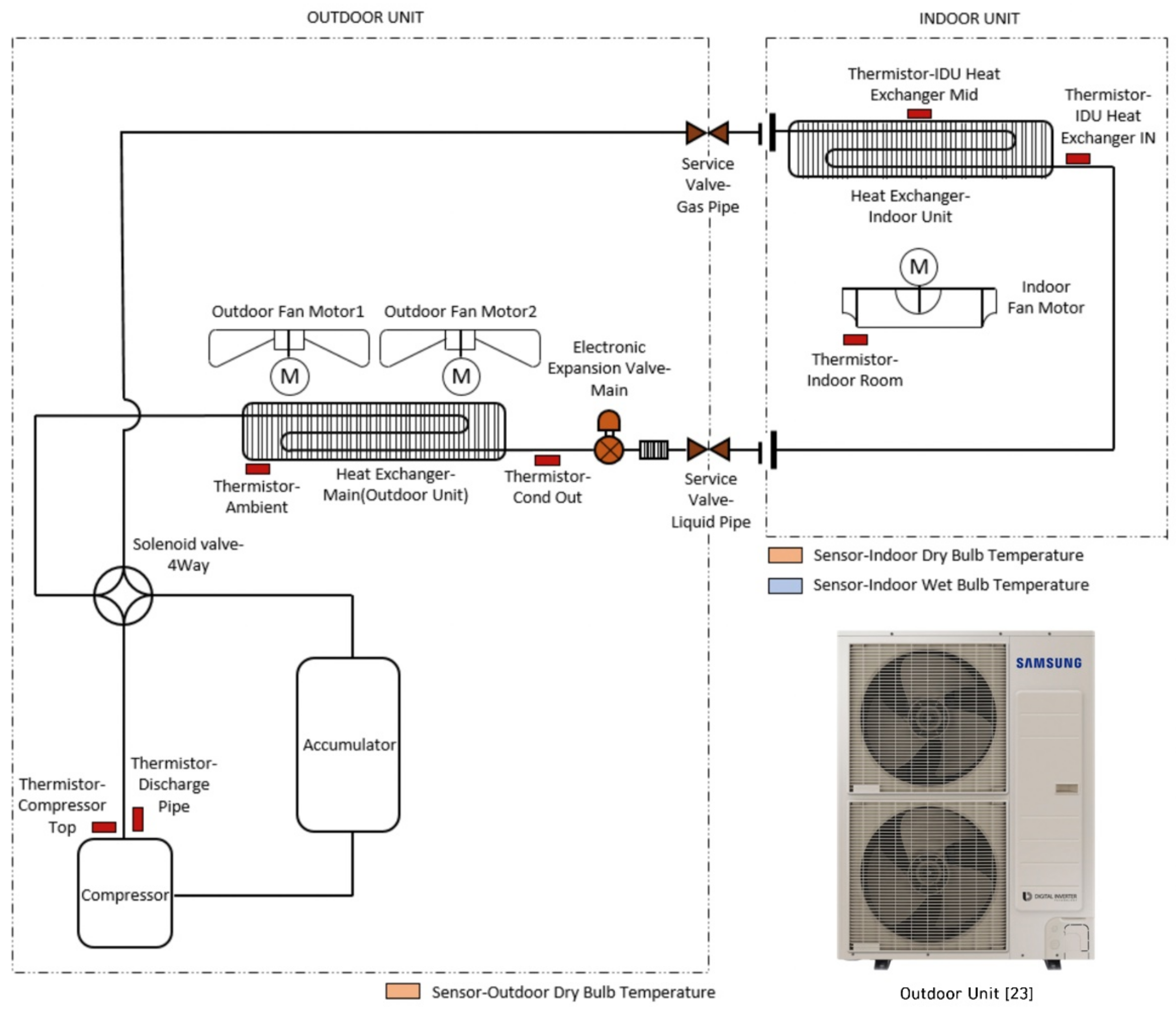
2.1.1. Electric Heat Pumps (EHPs)

The psychrometric calorimeter test facility comprised both indoor and outdoor chambers. The variables associated with refrigerant temperatures have been experimentally measured under variable experimental conditions in a psychrometric calorimeter test facility. Moreover, the specifications of the heat pump systems for both cooling and heating modes were identified. Regarding the EHP system used for training the model, Table 1 lists the capacity, power, and current for both cooling and heating. The system comprises indoor (Model number: AC145RN4PBH1) and outdoor units (Model number: AC145RX4PHH3). The operating temperature of the outdoor unit is −15–50 °C in the cooling mode and −25–24 °C in the heating mode. Moreover, the actual capacity of the compressor is 4.12 kW. In the EHP system, a liquid pipe with an internal diameter of 9.52 mm and a gas pipe having an internal diameter of 15.88 mm were installed. The refrigerant used in the system was R410a, one of the major alternatives to R22; moreover, an electronic expansion valve (EEV) was used to operate the refrigerant in the system.
Figure 1 shows the schematic of the EHP system for model development. It shows both physical connections and placement of the components such as the outdoor fan motors, indoor fan motors, heat exchangers, compressors, accumulators, and valves. Moreover, the valve types include EEVs used for refrigerant operation, four-way solenoid valve used for controlling the flow rate of the chilled water flowing into the heat exchanger, and service valves used for liquid and gas pipes. The four-way valve caused the chilled water to flow more into the heat exchanger when the ambient temperature increased. The heat exchangers were divided into the primary and sub heat exchangers; moreover, the temperature of the refrigerant at the inlet, inside, and the outlet were measured. Note that the system operates on a single compressor.
Using 204-type NTC thermistors, the temperature of the refrigerant at the outlet and top of the compressor was measured, and the refrigerant temperature at the condenser and heat exchanger were measured using 103-type NTC thermistors. As shown in Figure 1, the outdoor dry-bulb temperature, indoor dry-bulb temperature, and indoor wet-bulb temperature were measured, while the T-type thermocouples were used as measurement sensors. Table 2 lists the specifications of the experimental apparatus.
For testing the model, the capacity, power, and current of the EHP system were identified. Table 3 lists the minimum, standard, and maximum values for each specification. Table 3 also shows that the standard capacities of EHP systems for model training and testing have the same value; however, they differ in power consumption. The testing system comprises indoor (Model number: AC145JN4PBH1) and outdoor units (Model number: AC145KX4PHH3). The internal diameters of the liquid and gas pipes of the EHP system for the model testing were 9.52 and 15.88 mm, respectively; these values are equal to the diameters of the EHP system used for developing the model. For refrigerants, we used the same R410a used in the EHP system as that for model development.

2.1.2. Experimental Conditions

Under various RCAs, experimental conditions were set to measure variables associated with the compressor, condenser, and evaporator. Table 4 shows TOdB, TIdB, TIwB, and RCA values for each of the seven conditions from A to G. Under all experimental conditions, the undercharge, normal charge, and overcharge states of the RCA were set, and the states ranged from 60% to 120% with a 12% interval between successive states. Moreover, in the laboratory, the cooling mode of the EHP system was implemented. For most systems, the nominal RCA at rated conditions can be determined in the cooling mode [1,15]. Condition A–C show that TIdB is higher than TOdB, whereas conditions E–G show the state where the TOdB is higher than TIdB. For condition D, both TIdB and TOdB are set to 27 °C. As shown in Table 4, TOdB, TIdB, and ID WB ranged from 5 °C to 43 °C, 20 °C to 32 °C, and 15 °C to 27.5 °C, respectively. Moreover, most of the on-site installed EHP systems were found to be installed under the environmental condition of TOdB being < 40 °C. Under experimental conditions, the TOdB from 5 °C to 43 °C was used to predict RCA in a wider range compared to the temperature range readily accessible at most sites.

2.2. Data Collection

To easily apply the proposed approach in on-site systems, all experimental results were collected using sensors and data loggers. The data measurement interval of the sensors was 10 s. For the training dataset, in addition to the 42 static state data, 2381 dynamic state data were added to the training dataset; however, for the testing dataset, a total of 18 data were measured when the RCA was 60%, 70%, and 100%. Finally, the training dataset had 2423 entries while the testing datasets had 18 entries.
Table 5 lists the details of the 22 selected variables. These features were used as input variables to develop the DNN-based RCA prediction models. ΔTcond and ΔTcomp were calculated as the difference between the Tcond,out and TOdB and the difference between Tcomp,out and TOdB, respectively. The dataset for developing the basic DNN model was obtained based on the variables measured with the sensors. The thermodynamic properties of the refrigerant in the compressor, condenser, and evaporator were obtained using a thermodynamic model based on measured variables. For the compressor, the refrigerant temperature, pressure, enthalpy, entropy, and superheat at the inlet and outlet were estimated for model development. Note that refrigerant enthalpies at compressor outlet (hcomp,out, Scomp,out) were the values assumed to be isentropic. Scomp,out is the value obtained when 100% efficiency of the isentropic was applied. The superheat of refrigerant was calculated as the difference between the saturation temperature corresponding to the refrigerant pressure at the compressor outlet and Tcomp,out. Moreover, for the condenser, the pressure, enthalpy, and subcooling of the refrigerant at the outlet were calculated using the thermodynamic model. The subcooling of the refrigerant was calculated as the difference between saturation temperature, corresponding to refrigerant pressure at the compressor outlet and condenser outlet. Moreover, the dry-bulb temperature and the pressure of the refrigerant at the evaporator inlet were estimated; ΔP and Δh were calculated as the difference in the refrigerant pressure and enthalpy in the compressor, condenser, and evaporator. The variables measured under various experimental conditions and the thermodynamic properties obtained through the thermodynamic model using these variables constitute the dataset required for implementing the hybrid DNN model.

2.3. Thermodynamic Model

Thermodynamic properties such as pressure, density, heat capacity, enthalpy, and entropy, which are obtained through a thermodynamic model, are important for determining the performance of EHP systems. Moreover, they are required for simplifying equipment operation and design [24]. In this study, the National Institute of Standards and Technology (NIST) REFPROP program was used as a thermodynamic model to obtain the abovementioned properties. Moreover, this model is referred to as a white-box model because it clearly explains the influencing input variables and how the outcomes are obtained. The following sections explain the combination of this thermodynamic model with a DNN model to make a hybrid model that increases the number of variables and RCA prediction performance. The NIST REFPROP program, which has different coefficients and exponents for each mixture, uses the equation of state (EoS) to calculate the thermodynamic properties of RCA mixtures with different compositions. The calculated RCA values demonstrated that experimental data could be reproduced within the reliable experimental uncertainty of the data [25,26]. For thermodynamic properties such as density, the results conform with experimental data [27].
The EoS, expressed in terms of Helmholtz energy, has been extensively used as a reference equation to calculate the thermodynamic properties for multiple refrigerant mixtures [28]. The equations could be used to calculate the thermodynamic properties of the mixture in various compositions. These equations and their computational usage have been incorporated into the NIST REFPROP database. While properties obtained using fluid-specific correlations cannot be denied, NIST REFPROP proved to produce reliable performance [29]. The estimated uncertainties of calculated properties are 0.1% in density and 0.5% in heat capacity [30]. The NSIT REFPROP results showed good agreement compared with experimental data of Ar and C3H8 [31]. Kim and Shin [32] and Haung, Ding, Hu, et al. [33] confirmed the enthalpy, temperature, pressure, and mass flow values using NIST REFPROP. An error range of ±0.2% was discovered compared to experimental data. In this study, thermodynamic properties were calculated through mixture equations presented in NIST REFPROP by reflecting the characteristics of R32 and R125, which constitute the mixture R410a, which has received considerable attention and has been increasingly used as a working fluid in many air-conditioning and heat pump applications [34,35]. Appendix A presents the details of the thermodynamic model.

2.4. Deep Neural Network Model

2.4.1. Deep Neural Network (DNN)

To ensure the algorithm works better, traditional machine learning algorithms require the user’s knowledge about the data and the machine-learning algorithm. Moreover, these algorithms are prone to overfitting and less generalization ability because the data amount increases; however, deep learning has the potential to overcome drawbacks of using traditional machine learning algorithms by discovering the intricate structure in data sets using backpropagation algorithms [36,37]. Major advances in deep learning have been made for addressing challenges that have resisted the best attempts of the machine learning community for many years [38]. Using deep structures, rather than shallow ones, DNN is able to capture useful information from raw data and approximate complex non-linear functions with a small error [39]; hence, we adopted DNN in this study.
DNN models are capable of learning high complex patterns within the presented data and provide a scope for reducing the generalization error. Figure 2 shows a typical architecture of a DNN model, which is composed of one input layer, several hidden layers, and a single output layer. This architecture permits incremental learning and the layer-by-layer manner in which increasing complex representations are developed and jointly learned.
During the DNN training process, neurons weights and biases are updated and adjusted using the supervised learning backpropagation and optimization technique such as stochastic gradient descent [40]. The activation functions of hidden layers play a major role for mapping the nonlinear relationship between both input and output. Therefore, without the activation functions, non-linear patterns among variables cannot be learned [41]. The nonlinear activation function, f , is detailed in Equation (1). α represents the weighted combination and b represents activation thresholds of neurons. Both x i and w i represent the neuron’s input values and weights, respectively.
Of the activation functions, Rectifier, Tanh, and Maxout have recently been used for implementing the most accurate prediction performance in DNN and have been effectively applied [42]. The formula for Rectifier, Tanh, and Maxout are denoted as Equations (2), (3), and (4), respectively.
f α = f i = 1 n w i x i + b
  f α = max 0 , α
f α = e α e α e α + e α
  f α 1 , α 2 = max α 1 , α 2
To avoid overfitting and increase the generalizability in DNN, regularization techniques such as dropouts and weight regularizers are used. The use of dropouts is a technique where randomly selected neurons are ignored during the training process [43]. If the neurons randomly drop out during training, they are prevented from overlearning or co-adapting; consequently, the developed model has a low generalization error. Using L1 (Lasso) and L2 (Ridge), weight regularization can be achieved. These are used to add stability and improve generalization by setting the values of multiple weights to smaller values. L1 and L2 enforce penalties and modify the loss function by minimizing them [44,45]. The regularization process of L1 and L2 is denoted in Equation (5). The size of penalty is determined by hyperparameters λ 1 and λ 2 . R 1 W , B | j and R 2 W , B | j show the sum of the absolute values of weights and the sum of the squared weights, respectively. The penalty is performed by adding λ 1 R 1 W , B | j and λ 2 R 2 W , B | j to the result of loss function.
L W , B | j = L W , B | j + λ 1 R 1 W , B | j + λ 2 R 2 W , B | j

2.4.2. Model development

Figure 3 shows the developmental structure of basic DNN and hybrid DNN models that predict RCA for EHP systems. The basic DNN model is a typical black-box model developed with experimental modeling techniques that use only measured data. However, a hybrid DNN model is a gray-box model combining a black-box model and a white-box model. In addition to the measured data, the hybrid DNN model uses thermodynamic properties calculated using the thermodynamic model. The measured data are outdoor dry-bulb temperature (TOdB), indoor dry-bulb temperature (TIdB), refrigerant temperature at evaporation inlet (Tevap,in), refrigerant temperature at compressor outlet (Tcomp,out), and refrigerant temperature at condenser outlet (Tcond,out). Section 2.3 discusses the thermodynamic properties in detail. All data used for designing the models were collected from two EHP systems with different specifications. The data from one EHP was used for training, whereas that from the other EHP was used for testing. To remove missing and null values, data fitting was performed via statistical methods such as cumulative histogram, scatter plots, and box plots. The testing dataset was used to evaluate the performance and generalizability of the developed prediction models. The optimal parameters of DNN used for developing both prediction models were selected using a Cartesian random search. Parameters such as the number of hidden layers and activation functions were optimized using a random search; the process is discussed in Section 2.4.3 in detail. In terms of computational capacity, the workstation used for model development and testing has an NVIDIA GeForce GT 710 graphics processing unit (GPU), Intel® core™i5-7500 central processing unit (CPU) with a processor of 3.4GHz and a memory of 32GB. The computational time for model development was approximately 1 hour for the basic DNN model and 2 hours for the hybrid DNN model.

2.4.3. Model Optimization and Evaluation

For deep learning, the DNN hyperparameters required for achieving the model learning process can considerably affect model performance; however, because of the complexity of the data to be analyzed increased, tuning hyperparameters has become an intractable task [46]. These hyperparameters include the number of hidden layers, the number of neurons in each layer, the maximum number of epochs, loss function, optimizer, learning rate, and regularization method. A good model uses the optimal combination of these hyperparameters and achieves good generalization capability.
Using both manual and automatic approaches, DNN hyperparameters are adjusted [47]. The manual approach, which is tedious, is based on expert knowledge where the expert inspects how the hyperparameters affect the performance of the model. Moreover, the search space expands exponentially with respect to the number of hyperparameters. Automatic hyperparameter optimization uses algorithms that combine a list of the hyperparameters. Grid search and Random search are two popular algorithms. Grid search evaluates every model corresponding to each hyperparameters combination provided in the list, whereas Random search tries random combinations of the hyperparameters to identify the best model. This study used Random search because it helps identify models that are as good as the models obtained by Grid search within minimal computation time [47].
Previously, studies have reported a simple mathematical formula (Equation (6)) that determines the number of neurons in hidden layers [48,49]. Thus, Equation (6) was used to set the minimum number of neurons in the hyperparameters list in Random search for the basic and hybrid DNN models: 15 neurons and 45 neurons were obtained, and 7 and 22 inputs were used to develop the basic and hybrid DNN models, respectively.
Number of neurons = 2n + 1, n = number of inputs
For both DNN models, the number of hidden layers ranged from 2 to 6. The maximum number of epochs was set to 1000 epochs. The lists of activation functions included Rectifier, Tanh, and Maxout, and L1 and L2 regularization were used to identify the best regularizer.
The models were evaluated using the coefficient of determination (R2) and root mean squared error (RMSE). A good model uses the highest R2 and lowest RMSE in both the training and testing dataset. Equations (7) and (8) describe the calculations of R2 and RMSE, where y k and y k ^ are the actual and predicted values at step k, respectively.
  RMSE = k = 1 n ( y k y k ^ ) 2 n
R 2 = 1 k = 1 n y k y k ^ 2 k = 1 n y k y k ¯ 2

3. Results

3.1. Relationship between Measured Variables and RCA

The relationship between the measured variables and RCA under various experimental conditions was measured (Table 4) and discussed in Section 2.1.2. Table 6 shows the Pearson correlation coefficient (R) values between the measured variables and RCA. The value of R ranges from −1 to 1; the sign of the correlation coefficient indicates the direction of the relationship (positive or negative). The strength of the relationship is proportional to how close the R value is to −1 or 1. In this study, statistical significance was determined at P > 0.01; moreover, all the measured variables (i.e., Tevap,in, Tcond,out, Tcomp,out) correlated with RCA and the correlations were statistically significant (P > 0.001) except for the relationship between RCA and Tcomp,out under experimental condition B (R = 0.103, P < 0.001). Moreover, results showed that Tevap,in is positively correlated with RCA, whereas Tcond,out and Tcomp,out were negatively correlated with RCA under all experimental conditions. For example, under experimental condition A, R between RCA and Tevap,in, RCA and Cond, and RCA and Tcomp,out were 0.917, −0.477, and −0.894, respectively. To summarize, the strongest correlations were observed between RCA and Tevap,in, followed by RCA and Tcond,out and RCA and Tcomp,out. For example, R between RCA and Tevap,in were > 0.70 under all experimental conditions except for experimental conditions B, C, and E. Similarly, R between RCA and Tcond,out was > 0.70 under all experimental conditions except for experimental conditions B, C, and F. However, R between RCA and Tcomp,out was < 0.70 under all experimental conditions except for experimental conditions D, F, and G. Moreover, we observed that R between RCA and all the three measured variables (i.e., Tevap,in, Cond, Tcomp,out) was > 0.70 under experimental conditions D and G.

3.2. Prediction Performance

3.2.1. Random Search Results

For neural network-based algorithms, in each hidden layer, the number of neurons has considerable influence on the prediction performance of developed predictive models. Generally, the number of neurons in input and output layers is the same as the number of input and output variables, respectively; however, there are no standard rules for determining the appropriate number of neurons per hidden layer [50]. To determine the optimal number of neurons in each hidden layer, empirical approaches have been determined. Subsequently, studies have developed simple mathematical formula to determine the number of neurons in hidden layers (i.e., 2n + 1) [48,49]. In this study, such a formula was used to determine the minimum number of neurons in hidden layers. Based on the formula, the minimum number of neurons for the basic DNN model (7 input variables) and hybrid DNN model (i.e., 22 input variables) at 15 and 45 neurons were determined. For the basic DNN model, the initial setting of the parameters model was as follows: the L1 regularization was set to 1 × 10⁻³, the L2 regularization was set to 1 × 10⁻³, the number of epochs was set to 1000, and the activation function was set to Rectifier. Subsequently, a 5-layer DNN model that included input and output layers was developed. For this model, the number of neurons was set to 15 neurons based on the abovementioned formulae. We then iteratively increased the number of neurons by 15 until there was no further increase in R2 or a decrease in RMSE. For the 5-layer DNN, the optimum performance was found with 75 neurons in the second and second to the last hidden layers and 150 neurons in the middle layer. These conditions were maintained as the number of hidden layers was increased; consequently, for all the developed models, the number of neurons in the second and second to the last hidden layers was 75, whereas the neurons in the middle layers were maintained at 150 neurons. Consequently, the hidden layers composed of combinations based on 75 and 150 neurons were used for the random search. In the random search, hidden layers and training scheme were optimized as follows: (1) the number of hidden layers (ranging from 2 to 7); (2) the activation function (including Rectifier, Tanh, and Maxout); (3) the L1 regularization (0, 1e-4, and le-6); and (4) the L2 regularization (0,1e-4, and le-6). For the activation function, the Rectifier function is the most extensively used; however, Maxout and Tanh were used for random search to evaluate the change of model prediction performance by various activation functions. For the hybrid DNN model, the number of neurons was maintained as mentioned previously. Moreover, the range of parameters determined for the random search was set to the same value as that of the basic DNN model.
Table 7 shows random search results for both basic DNN and hybrid DNN models. Table 7 shows the top five models with a high prediction performance using R2 and RMSE values among the models developed via a random search. Moreover, it presents the parameters optimized using random search. For the basic DNN model, a model developed with Rectifier and two hidden layers showed optimal prediction performance. Moreover, models developed using Maxout as an activation function showed a relatively high R2 value; however, models using Tanh as an activation function showed a reduced predictive performance regardless of the number of hidden layers. In addition to the basic DNN model, the hybrid DNN model was found to have a relatively reliable predictive performance when using Rectifier and Maxout as activation functions. Most models developed using Rectifier and Maxout functions had satisfactory R2 values of > 0.8 regardless of the number of hidden layers. In particular, models developed with Rectifier as an activation function and using three and six hidden layers, respectively, had R2 values of > 0.9.
For both basic and hybrid DNN models, models developed with Rectifier showed very reliable prediction performance. Rectifier, which has good sparsity properties because of its real zero value and can represent any non-negative real value, has recently been proposed as an efficient activation function [51]. Moreover, the Rectifier function has been effectively applied to DNN-based prediction modeling [42,51]. Furthermore, we reported that when not using “dropout” as a parameter, models developed with Maxout, which works by multiplying the input vector by a matrix, has relatively lower predictive performance compared to models developed using the Rectifier function. Furthermore, compared to the models developed with Rectifier and Maxout functions, models developed with Tanh have a low predictive performance. This may be attributed to Tanh being a type of sigmoidal activation function bounded by minimum and maximum values, thus causing saturated neurons in the higher layers of the neural networks. Consequently, these saturated neurons limit the depth of the neural network that can be trained.

3.2.2. Prediction Performance on Training Dataset

Figure 4 shows the prediction performance of the developed basic DNN model and hybrid DNN model under each experimental condition using the training dataset. The x-axis represents the number of data points and the y-axis represents RCA. The basic DNN and hybrid DNN models can explain the reason for 96% and 99% of total variance in RCA, respectively. The prediction performance of developed models differed according to experimental conditions. However, on an average, the basic DNN model showed a predictive performance of 95%, whereas the hybrid DNN model showed a high predictive performance of 99% under all conditions except condition A. For the basic DNN model, the prediction performance was relatively low for experimental conditions A and G; however, it had a high prediction performance of >98% at experimental conditions B, C, D, and E. Figure 4 shows that, especially under the experimental condition E, the values predicted through both developed models were highly similar to measured values.
According to the indoor and outdoor temperature, the experimental conditions can be classified into three types of cases: the first case indicates conditions when TIdB is higher than TOdB, the second case indicates conditions when TIdB and TOdB are the same, and the third case indicates conditions when TOdB is higher than TIdB. The developed models showed a higher predictive performance under the second case compared to the first and third cases. The developed basic DNN and hybrid DNN models, under the second case (i.e., TIdB greater than TOdB), could explain the reason for the 98% and 99% of the total variance in RCA, respectively. Moreover, the difference in the predictive accuracy between the basic DNN model and the hybrid DNN model under the first and second cases was < 1%. However, under the third class, the predictive accuracy of the hybrid DNN model was 4% higher compared to the basic DNN model.
Figure 5 shows the RMSE values of development models according to RCA. As shown in Figure 5, the RMSE gap between the developed models increased as the charge amount increased under conditions when the charge state is > 84%. The difference in the performance of the two models was better observed when the RCA was in an overcharge state (i.e., 120%). Moreover, the lowest RMSE values of 0.0176 and 0.0143 for the basic DNN model and hybrid DNN model, respectively, were observed at the RCA of 84%. Furthermore, the hybrid DNN model had a RMSE value of <0.04 at all charge states and showed the lowest RMSE value of 0.006 at a charge state of 108%.

3.2.3. Prediction Performance of Testing Datasets

Figure 6 shows the prediction performance of basic DNN and hybrid DNN models. The y-axis shows the RMSE and R2 values for each model. The results obtained using both training and testing datasets show that the hybrid DNN model had a relatively higher R2 value and relatively lower RMSE value compared to the basic DNN model. For the training dataset, the basic DNN model had an R2 value of 0.9646 and a RMSE value of 0.0426; however, the hybrid DNN model had an R2 value of 0.9913 and a RMSE value of 0.0197. For the testing dataset, the basic DNN model had an R2 value of 0.7217 and a RMSE value of 0.0797, whereas the hybrid DNN model had an R2 value of 0.9312 and a RMSE value of 0.0395. As shown in Figure 6, the prediction performance for the testing dataset is relatively lesser than that for the training dataset for both models; however, the difference between the predictive performance using the training and testing dataset was larger for the basic DNN model compared to the hybrid DNN model. For example, the difference in prediction performance between the training dataset and the testing dataset was 24% and 6% for the basic DNN model and the hybrid DNN model, respectively.
Table 8 shows predictive values of models developed using the testing dataset. Because of verification of the standard deviation of the error between the predicted values and the measured values, the basic DNN model and the hybrid DNN model had values of 11% and 6%, respectively. The performance of the developed models under the three categories of the experimental conditions was analyzed; the first case was when TIdB is higher than TOdB, the second case was when TIdB and TOdB are the same, and the third case was when TOdB is higher than TIdB. The basic DNN model performed better (R2 = 96%) under the third class (TOdB > TIdB) compared to the first case (TOdB < TIdB) where R2 = 87%. Similarly, the hybrid DNN model showed a better predictive performance under the third case (R2 = 97%) compared to the first case (R2 = 94%).
For model testing, RCA was set to 60%, 70%, and 100%. Both developed models had the smallest RMSE error at a charge state of 60% and the largest RMSE at a charge state of 70%. The basic DNN and hybrid DNN models had RMSE of 6.27% and 1.47% at a charge of 60%, 8.41% and 4.73% at a charge of 70%, and 7.58% and 4.6% at a charge of 100%, respectively. Moreover, the hybrid DNN model had a smaller RMSE compared to the basic DNN model in all charge states.

4. Discussion

This study reports a hybrid DNN model for predicting the RCA of heat pumps by incorporating a DNN model and a thermodynamic model. The values predicted using a hybrid DNN model agreed with the measured values. Recently, estimating the RCA in EHP systems has attracted considerable interest [15,52]. However, because of the difficulty in developing an appropriate physics-based estimation model, most estimation algorithms developed in existing studies rely on experimental modeling [52,53]. The developed physics-based mathematical algorithms showed relatively good prediction performance with a relative deviation of 8.0% [13]; however, they are often designed for individual systems and have problems with time and implementation costs. In this study, DNN-based experimental modeling was performed for RCA prediction using variables measured from on-site installed systems. Furthermore, a hybrid DNN model using thermodynamic properties obtained through the theoretical-based thermodynamic model was developed. The hybrid DNN model predicted RCA with a reliable accuracy of 97% under all seven experimental conditions with different set indoor and outdoor dry-bulb temperature.
RCA is an important optimization parameter in the EHP system because it considerably affects the coefficient of performance (COP) and the energy efficiency of the systems positively; therefore, it needs to be intensively controlled [7,8]. Moreover, because of the emergence of improving the energy efficiency of VRF systems using a technology built on direct expansion heat pump platform [54,55], efficient detection and control of RCA is essential. To efficiently control RCA, understanding the exact amount under various conditions is important. However, except for developing VRC sensors, very few studies have estimated the exact RCA. However, most studies have focused on developing the FDD strategy to diagnose fault situations of the EHP system because of faulty RCA via ANN-based learning [20,21,56]. Moreover, the primary content of diagnosis for fault-related situations is determining the charge conditions such as undercharge and overcharge [19,21]. In this study, under a wide range of operating conditions by changing indoor and outdoor temperatures, the exact RCA was predicted. A RMSE value of <0.04 for all charge states, such as undercharge, normal charge, and overcharge, was confirmed using a developed model. According to various operating conditions, this approach can be used as part of an installed control or monitoring system to predict optimal RCA.
Another contribution of this study is related to variables used to study and estimate RCA. Previously, studies have examined RCA using factors such as outdoor dry bulb temperature and factors related to subcooling and superheating. These factors are important for estimating RCA, e.g., the outdoor dry-bulb temperature is essential for determining the fan step of the outdoor unit; therefore, it has considerable influence on the refrigerant flow in the EHP system [57]. Similarly, both subcooling and superheating have been reported to significantly affect RCA [2,13,58]. In addition to factors affecting RCA identified in previous studies [2,13,57,58], this study reveals the effects of three additional factors (i.e., Tevap,in, Tcond,out, and Tcomp,out) on RCA and shows the relationship between RCA and these factors under diverse experimental conditions (Section 3.1). Generally, the RCA was considerably affected by the refrigerant temperature at the evaporator inlet compared to the refrigerant temperature at compressor and condenser outlets. Furthermore, refrigerant temperature at evaporator inlet was positively correlated to RCA, whereas refrigerant temperature at both compressor and condenser outlets was negatively correlated to RCA. This information is useful for developing predictive models to estimate RCA. One important process for developing predictive models is the feature selection process; a process that involves determining important factors to be used as explanatory variables for training the model. In this study, the importance of refrigerant temperature at evaporator inlet, compressor outlet, and condenser outlet for estimating RCA was identified and validated. Therefore, future studies on the prediction of RCA should consider these factors (i.e., Tevap,in, Tcond,out and Tcomp,out) for developing RCA-predictive models.
In this study, the dynamic state data, which may occur during the operation lifecycle of the commercialized EHP system, were used for the development of the RCA prediction model. The transient nature of the external inputs to EHP systems resulted in dynamic fluctuations of system variables. Changes in room temperature and operations of components in the system, such as compressors and fans, induced transient responses [52]. Therefore, diagnosing the system fault through RCA prediction at various states such as the dynamic state of the EHP system to be commercialized is important. In particular, dynamic state data play an important role for accurate RCA prediction in an EHP system in which an accumulator is installed. However, the VRC sensor has been reported to have difficulty in estimating RCA for systems using accumulators [18]. When the EHP system is not running at a low outdoor temperature, the overcharged refrigerant is stored within the accumulator. Subsequently, the refrigerant stored in the accumulator was not easily released even if the compressor was restarted and changed to a dynamic state. Note that the VRC sensor made an error and detected this situation as a refrigerant shortage [12]. This study was conducted in EHP system equipped with the accumulator and reflected the following experimental conditions: (1) various states of RCA including undercharge and overcharge; (2) a wide range of temperature conditions, including outdoor temperature from as low as 5 °C to as high as 43 °C; and (3) experimental data measured in dynamic states before reaching the set experimental conditions. Consequently, the developed RCA hybrid DNN prediction model can cope with various circumstances in an on-site installed EHP system; hence, it confirms the high prediction performance.
To deal with the overfitting and generalization issues, RCA was predicted by applying a hybrid DNN model that combines a DNN model and a thermodynamic model to a system having a completely different specification from the EHP system in which the data used in the model development were measured. ANN has been continuously used in studies based on FDD for detecting faulty RCA [19,20,21,56]. Although the ANN has achieved considerable success in the refrigerant field, it still has a risk of poor generalization ability and overfitting [21,22]. When overfitting occurs, the developed model shows good performance for training data but poor generalization to data acquired from other systems. In this study, the basic DNN model, a type of black-box model based on experimental modeling, was developed using only measured data and showed poor generalization ability because of overfitting. It had a prediction performance of 96% and 72% for model training and model testing, respectively; however, the hybrid DNN model uses thermodynamic properties calculated through the thermodynamic model, a type of white-box model based on theoretical modeling, as additional input variables for model development. The hybrid DNN model had reliable prediction performance and showed outstanding generalization ability. For model training, it had a RMSE value of 0.0197 and an R2 value of 0.9913. For model testing, it had a RMSE value of 0.0395 and an R2 value of 0.9312. Consequently, a new approach to RCA prediction developed in this study shows that DNN and the thermodynamic model can be efficiently applied to overcome overfitting and poor generalization abilities.
To determine optimal parameters for DNN model development, hidden layers and training attributes were determined using random search. Parameters such as the number of hidden layers, the number of neurons in each layer, the number of epochs, and activation functions have considerable influence on the prediction performance of the DNN model [48,49,50]. However, determining optimal parameters for various models is important, and it is tedious to verify the number of all cases using the trial and error method. The random search is an efficient parameter selection method that provides developers optimal parameters that are suited for their model. It confirms the minimum error value for the models developed for all parameter combinations. In this study, the number of hidden layers and activation function optimized for DNN models were identified. First, the number of hidden layers (ranging from 2 to 7) and the activation function (Rectifier, Tanh, and Maxout) were specified for various sets to be researched. Various combinations were then compared and analyzed. Consequently, Rectifier was confirmed to be an optimized activation function for both the basic DNN model and the hybrid DNN model, and the optimized number of hidden layers was determined to be 2 and 3, respectively. The random search saved time compared to the trial and error method and was able to efficiently identify more various combinations of parameters.
The main practical challenge of our proposed approach is how efficiently it can be generalized to other systems. The thermodynamic properties used for developing the hybrid model were obtained based on the NIST REFPROP program, but the applicability of this program in on-site systems with real-time responses should be investigated. In addition, it is important to note that there are systems that already measure thermodynamic properties through sensors. When applying the proposed approach hybrid model, care should be taken to check its suitability for the prediction of energy demand and COP of EHP systems. If the model can predict energy demand and COP, along with the RCA of an EHP system, then it is expected to play an important role in terms of system optimization by reducing energy consumption, improving the system efficiency, and maintaining thermal comfort of the occupants. Further research on the main challenges mentioned above should be undertaken, thereby ensuring the generalizability of the proposed approach.
Future directions to be considered would be to test the hybrid DNN model after obtaining sufficient data from on-site EHP systems. This enables us to identify the generalizability of our approach. One of the major challenges is how to effectively collect a comprehensive dataset for model testing in terms of cost and time. This challenge could be partially overcome with the use of transfer learning. Transfer learning is the application of a pre-trained model during the execution of a primary task to the execution of a new but similar secondary work [59]. Through transfer learning, our model based on experimental data could be applied to each EHP system without developing a new model. Existing previous studies that used transfer learning have found it to be able to obtain faster and more cost-effective results under the process of a model test [60,61].

5. Conclusions

This study, which applies the DNN and a thermodynamic model, presents a highly efficient hybrid DNN model that predicts RCA under various temperature conditions. The measured data from two different EHP systems were used for training and testing of the models. Furthermore, the prediction performance of the hybrid DNN model was compared with the basic DNN model developed with only measured variables without using thermodynamic properties. Based on the results, the following conclusions were drawn:
(1)
The temperature variables such as indoor and outdoor dry-bulb temperature; the refrigerant temperature at the evaporator inlet, compressor outlet, and condenser outlet; and the difference between outdoor dry-bulb temperature and refrigerant temperature at outlets of compressor and condenser are used as input variables for the basic DNN model. For the hybrid DNN model, the thermodynamic properties, enthalpy, entropy, pressure, superheat, and subcooling, were used as additional input variables.
(2)
For DNN models developed in this study, the hidden layers and training scheme were optimized using random search. The basic DNN model and hybrid DNN model developed with optimized parameters have two and three hidden layers, respectively, and having the Rectifier as the activation function in common.
(3)
The new sophisticated RCA prediction model (hybrid DNN model) achieved high accuracy compared to the basic DNN model. For model testing, the RCA was predicted with a precision of 72% for the basic DNN model and 93% for the hybrid DNN model.
(4)
Under various experimental conditions, reliable prediction performance was confirmed with the hybrid DNN model. For model training, it had an average RMSE error of 2.93% for seven conditions that reflect different indoor and outdoor temperatures and a RMSE of 3.95% for testing.
(5)
The hybrid DNN model showed similar trends under various experimental conditions. For both training and testing, it had a high predictive performance at a normal charged state (~100%) than at an undercharged state (~70%). Moreover, it showed higher accuracy in conditions where outdoor dry-bulb temperature was relatively higher than the indoor dry-bulb temperature.
(6)
Overfitting and poor generalization challenges, which were identified as the problems of conventional ANN, were addressed by the hybrid DNN model. When the developed model was applied to the new EHP system, the RCA prediction performance decreased by 24% in the basic DNN model but recorded a decrease of 6% only in the hybrid DNN model. The prediction performance for model training was 99% and 93% for model testing.
The new approach implemented by combining DNN and the thermodynamic model proved to be an efficient strategy for RCA prediction in EHP systems. Applying the developed model to commercial EHP systems may be a good solution for solving the problems that can be attributed to the faulty RCA operations such as thermal discomfort for the occupants, lower COP, and equipment damage. In addition, the model, which can efficiently predict RCA with insufficient data, can be applied to new EHP systems.

Author Contributions

Conceptualization, G.Y.Y. and S.L.; Formal analysis, P.N.D. and M.S.; Investigation, J.K.H.; Methodology, G.Y.Y., S.L. and M.S.; Validation, M.S.; Visualization, J.K.H. and P.N.D.; Writing—original draft, J.K.H. and G.Y.Y.; Writing—review & editing, G.Y.Y., S.L., H.S., I.K. and M.S. All authors have read and agreed to the published version of the manuscript.

Funding

This research was supported by a grant (20AUDP-B127891-04) from the Architecture & Urban Development Research Program funded by the Ministry of Land, Infrastructure and Transport of the Korean government.

Conflicts of Interest

The authors declare no conflict of interest.

Appendix A. The Details of the Thermodynamic Model

The process presented in NIST REFPROP uses generalized equations, applicable to several mixtures, based on their corresponding states theory and using reducing parameters that are dependent on the mole fractions of the mixture [30]. The reducing parameters were used to modify the values of density and temperature for the mixture. Consequently, equations that use density, temperature, and composition as independent variables can identify thermodynamic properties using simple derivatives. Table A1 lists the equations for the mixture.
The sum of Helmholtz energy for an ideal mixture (aidmix) and Helmholtz energy for an excess property of a mixture (aE), which are defined as the actual mixture property is the mixture Helmholtz energy (a). The ideal gas Helmholtz energy ( a i 0 ) and residual Helmholtz energy ( a i r ) for aidmix calculations and coefficients and exponents of excess function for the mixture Helmholtz energy have been confirmed in a previous study by Lemmon and Jacobsen [62] Table A2 lists the coefficients and exponents of the mixture equations. Moreover, for the mixture equations of R410a, ζ i j , ξ i j , and Fij values are 28.95, −0.006008, and 1, respectively. The values of pressure, enthalpy, and entropy used for model development in this study are based on equations in Table A1. Table A3 and Table A4 show the list of physical quantities and the list of superscripts and subscripts, respectively.
Table A1. Equations of thermodynamic properties.
No.ValuesEquations
1Helmholtz energy (a) a = a idmix + a E
2Helmholtz energy for an ideal mixture
(aidmix)
a idmix = i = 1 m x i [ a i 0 ρ , T + a i r δ , τ + RTlnx i ]
3Reduced values of density (δ) δ = ρ / ρ red
4Reduced values of temperature (τ) τ = T red / T
5Reducing values of density (ρred) ρ red = i = 1 m x i ρ c i + i = 1 m 1 j = i + 1 m x i x j ξ ij 1
6Reducing values of temperature (Tred) T red = i = 1 m x i T c i + i = 1 m 1 j = i + 1 m x i x j ζ i j
7Excess function for the mixture
Helmholtz energy
a E RT = a E δ , τ , x = i = 1 m 1 j = i + 1 m x i x j F ij k N k δ d k τ t k exp δ l k
8Compressibility factor (Z), Pressure (p) Z = p ρ RT = 1 + δ α r δ τ
9Internal energy (u) u RT = τ α 0 τ δ + α r τ δ
10Enthalpy (h) h RT = τ α 0 τ δ + α r τ δ + δ α r δ τ + 1
11Entropy (s) s R = τ α 0 τ δ + α r τ δ α 0 α r
12Gibbs energy (g) g RT = 1 + α 0 + α r + δ α r δ τ
13Isochoric heat capacity (cv) c v R = τ 2 2 α 0 τ 2 δ + 2 α r τ 2 δ
14Isobaric heat capacity (cp) c p R = c v R + 1 + δ α r δ τ δ τ 2 α r δ τ 2 1 + 2 δ α r δ τ + δ 2 2 α r δ 2 τ
15Speed of sound (w) w 2 M RT = c p c v 1 + 2 δ α r δ τ + δ 2 2 α r δ 2 τ
16First derivative of pressure with respect
to density at constant temperature
p ρ T = RT 1 + 2 δ α r δ τ + δ 2 2 α r δ 2 τ
17Second derivative of pressure with
respect to density at constant
temperature
2 p ρ 2 T = RT ρ 2 δ α r δ τ + 4 δ 2 2 α r δ 2 τ + δ 3 3 α r δ 3 τ
18First derivative of pressure with respect
to temperature at constant density
p ρ ρ = R ρ 1 + δ α r δ τ δ τ 2 α r δ τ
19Ideal gas Helmholtz energy (α0) α 0 = i = 1 m x i a i 0 ( ρ , T ) RT + lnx i
20Residual Helmholtz energy (αr) α r = i = 1 m x i a i r δ , τ + α E ( δ , τ , x )
Table A2. Coefficients and exponents of the mixture equations.
kNktkdklk
1−0.007 29554.521
20.078 0350.5751
30.610 071.912
40.642 461.232
50.014 9650.592
6−0.340 492.623
70.085 65811.433
8−0.064 4294.563
Table A3. List of physical quantities.
AbbreviationPhysical QuantityUnit
aMolar Helmholtz energyJ/mol
AHelmholtz energyJ
cpIsobaric heat capacityJ/(mol∙K)
cvIsochoric heat capacityJ/(mol∙K)
dDensity exponent
fFugacityMPa
FGeneralized factor
gGibbs energyJ/mol
hEnthalpyJ/mol
lDensity exponent
mNumber of components
MMolar massg/mol
nNumber of molesmol
pPressureMPa
RMolar gas constantJ/(mol∙K)
sEntropyJ/(mol∙K)
tTemperature exponent
TTemperatureK
uInternal energyJ/mol
vMolar volumedm3/mol
VVolumedm3
wSpeed of soundm/s
xCompositionmole fraction
ZCompressibility factor (Z = p/ρRT)
αReduced Helmholtz energy (α = a/RT)
δReduced density (δ = ρ/ρc)
ρMolar densitymol/dm3
τInverse reduced temperature (τ = Tc/T)
μChemical potentialJ/mol
ξReduced density parameterdm3/mol
ζReduced temperature parameterK
kNktkdklk
1−0.007 29554.521
20.078 0350.5751
30.610 071.912
40.642 461.232
50.014 9650.592
6−0.340 492.623
70.085 65811.433
8−0.064 4294.563
Table A4. List of superscripts and subscripts.
Superscripts Superscripts
0Ideal gas property0Reference state property
EExcess propertyCCritical point property
idmixIdeal mixturecalcCalculated using an equation
rResidualdataExperimental value
Saturated liquid statei,jProperty of component i or j
Saturated vapor stateredReducing parameter

References

  1. Choi, J.M.; Kim, Y.C. The effects of improper refrigerant charge on the performance of a heat pump with an electronic expansion valve and capillary tube. Energy 2002, 27, 391–404. [Google Scholar] [CrossRef]
  2. Tassou, S.A.; Grace, I.N. Fault diagnosis and refrigerant leak detection in vapour compression refrigeration systems. Int. J. Refrig. 2005, 28, 680–688. [Google Scholar] [CrossRef]
  3. Akkurt, G.G.; Aste, N.; Borderon, J.; Buda, A.; Calzolari, M.; Chung, D.; Costanzo, V.; Del Pero, C.; Evola, G.; Huerto-Cardenas, H.E.; et al. Dynamic thermal and hygrometric simulation of historical buildings: Critical factors and possible solutions. Renew. Sustain. Energy Rev. 2020, 118, 109509. [Google Scholar] [CrossRef]
  4. Serraino, M.; Lucchi, E. Energy Efficiency, Heritage Conservation, and Landscape Integration: the Case Study of the San Martino Castle in Parella (Turin, Italy). Energy Procedia 2017, 133, 424–434. [Google Scholar] [CrossRef]
  5. Choi, J.; Kim, Y. Influence of the expansion device on the performance of a heat pump using R407C under a range of charging conditions. Int. J. Refrig. 2004, 27, 378–384. [Google Scholar] [CrossRef]
  6. Cho, H.; Ryu, C.; Kim, Y.; Kim, H.Y. Effects of refrigerant charge amount on the performance of a transcritical CO2 heat pump. Int. J. Refrig. 2005, 28, 1266–1273. [Google Scholar] [CrossRef]
  7. Kim, W.; Braun, J.E. Impacts of Refrigerant Charge on Air Conditioner and Heat Pump Performance. In Proceedings of the 13th International Refrigeration and Air Conditioning Conference, West Lafayette, IN, USA, 10–15 July 2010; pp. 1–8. [Google Scholar]
  8. Kim, W.; Braun, J.E. Evaluation of the impacts of refrigerant charge on air conditioner and heat pump performance. Int. J. Refrig. 2012, 35, 1805–1814. [Google Scholar] [CrossRef]
  9. Downey, T.; Proctor, J. What Can 15,000 Air Conditioners Tell Us. Available online: https://www.proctoreng.com/dnld/biasedresultsairflow.pdf (accessed on 5 April 2020).
  10. Salmon, W. Review of recent commercial roof top unit field studies in the practice northwest and California. Available online: https://newbuildings.org/sites/default/files/NWPCC_SmallHVAC_Report_R3_.pdf (accessed on 5 April 2020).
  11. Li, Z.; Tan, J.; Li, S.; Liu, J.; Chen, H.; Shen, J.; Huang, R.; Liu, J. An efficient online wkNN diagnostic strategy for variable refrigerant flow system based on coupled feature selection method. Energy Build. 2019, 183, 222–237. [Google Scholar] [CrossRef]
  12. Kim, W.; Braun, J.E. Performance evaluation of a virtual refrigerant charge sensor. Int. J. Refrig. 2013, 36, 1130–1141. [Google Scholar] [CrossRef]
  13. Choi, H.; Cho, H.; Choi, J.M. Refrigerant amount detection algorithm for a ground source heat pump unit. Renew. Energy 2012, 42, 111–117. [Google Scholar] [CrossRef]
  14. Hu, Y.; Li, G.; Chen, H.; Li, H.; Liu, J. Sensitivity analysis for PCA-based chiller sensor fault detection. Int. J. Refrig. 2016, 63, 133–143. [Google Scholar] [CrossRef]
  15. Li, G.; Hu, Y.; Chen, H.; Shen, L.; Li, H.; Li, J.; Hu, W. Extending the virtual refrigerant charge sensor (VRC) for variable refrigerant flow (VRF) air conditioning system using data-based analysis methods. Appl. Therm. Eng. 2016, 93, 908–919. [Google Scholar] [CrossRef]
  16. Li, H.; Braun, J. Virtual Refrigerant Pressure Sensors for Use in Monitoring and Fault Diagnosis of Vapor-Compression Equipment. HVAC&R Res. 2009, 15, 597–616. [Google Scholar]
  17. Lin, X.; Lee, H.; Hwang, Y.; Radermacher, R. A review of recent development in variable refrigerant flow systems. Sci. Technol. Built Environ. 2015, 21, 917–933. [Google Scholar] [CrossRef]
  18. Kim, W.; Braun, J.E. Evaluation of a Virtual Refrigerant Charge Sensor. Available online: https://digitalcommons.unl.edu/cgi/viewcontent.cgi?article=1139&context=archengfacpub (accessed on 5 April 2020).
  19. Guo, Y.; Li, G.; Chen, H.; Wang, J.; Guo, M.; Sun, S.; Hu, W. Optimized neural network-based fault diagnosis strategy for VRF system in heating mode using data mining. Appl. Therm. Eng. 2017, 125, 1402–1413. [Google Scholar] [CrossRef]
  20. Son, J.E.; Nam, S.; Kang, K.; Lee, J. Refrigerant Charge Estimation for an Air Conditioning System using Artificial Neural Network Modelling. In Proceedings of the 2018 18th International Conference on Control, Automation and Systems (ICCAS), Daegwallyeong, South Korea, 17–20 October 2018. [Google Scholar]
  21. Shi, S.; Li, G.; Chen, H.; Liu, J.; Hu, Y.; Xing, L.; Hu, W. Refrigerant charge fault diagnosis in the VRF system using Bayesian artificial neural network combined with ReliefF filter. Appl. Therm. Eng. 2017, 112, 698–706. [Google Scholar] [CrossRef]
  22. Shi, S.; Li, G.; Chen, H.; Hu, Y.; Wang, X.; Guo, Y.; Sun, S. An efficient VRF system fault diagnosis strategy for refrigerant charge amount based on PCA and dual neural network model. Appl. Therm. Eng. 2018, 129, 1252–1262. [Google Scholar] [CrossRef]
  23. Samsung. Available online: https://www.samsung.com/sec/support/model/AC145KX4PHH3/ (accessed on 5 April 2020).
  24. Mora R, J.E.; Pérez T, C.; González N, F.F.; Ocampo D, J.D.D. Thermodynamic properties of refrigerants using artificial neural networks. Int. J. Refrig. 2014, 46, 9–16. [Google Scholar] [CrossRef]
  25. Sieres, J.; Varas, F.; Martínez-Suárez, J.A. A hybrid formulation for fast explicit calculation of thermodynamic properties of refrigerants. Int. J. Refrig. 2012, 35, 1021–1034. [Google Scholar] [CrossRef]
  26. Thol, M.; Lemmon, E.W. Equation of State for the Thermodynamic Properties of trans-1,3,3,3-Tetrafluoropropene [R-1234ze(E)]. Int. J. Thermophys. 2016, 37, 1–16. [Google Scholar] [CrossRef]
  27. Coquelet, C.; El Abbadi, J.; Houriez, C. Prediction of thermodynamic properties of refrigerant fluids with a new three-parameter cubic equation of state. Int. J. Refrig. 2016, 69, 418–436. [Google Scholar] [CrossRef]
  28. Al Ghafri, S.Z.S.; Rowland, D.; Akhfash, M.; Arami-Niya, A.; Khamphasith, M.; Xiao, X.; Tsuji, T.; Tanaka, Y.; Seiki, Y.; May, E.F.; et al. Thermodynamic properties of hydrofluoroolefin (R1234yf and R1234ze(E)) refrigerant mixtures: Density, vapour-liquid equilibrium, and heat capacity data and modelling. Int. J. Refrig. 2019, 98, 249–260. [Google Scholar] [CrossRef]
  29. Fouad, W.A.; Vega, L.F. Transport properties of HFC and HFO based refrigerants using an excess entropy scaling approach. J. Supercrit. Fluids 2018, 131, 106–116. [Google Scholar] [CrossRef]
  30. Lemmon, E.W.; Jacobsen, R.T. Equations of State for Mixtures of R-32, R-125, R-134a, R-143a, and R-152a. J. Phys. Chem. Ref. Data 2004, 33, 593–620. [Google Scholar] [CrossRef] [Green Version]
  31. Velasco, S.; Santos, M.J.; White, J.A. Extended corresponding states expressions for the changes in enthalpy, compressibility factor and constant-volume heat capacity at vaporization. J. Chem. Thermodyn. 2015, 85, 68–76. [Google Scholar] [CrossRef]
  32. Kim, M.-H.; Shin, J.-S. Evaporating heat transfer of R22 and R410A in horizontal smooth and microfin tubes. Int. J. Refrig. 2005, 28, 940–948. [Google Scholar] [CrossRef]
  33. Huang, X.; Ding, G.; Hu, H.; Zhu, Y.; Peng, H.; Gao, Y.; Deng, B. Influence of oil on flow condensation heat transfer of R410A inside 4.18mm and 1.6mm inner diameter horizontal smooth tubes. Int. J. Refrig. 2010, 33, 158–169. [Google Scholar] [CrossRef]
  34. Kong, X.Q.; Li, Y.; Lin, L.; Yang, Y.G. Modeling evaluation of a direct-expansion solar-assisted heat pump water heater using R410A. Int. J. Refrig. 2017, 76, 136–146. [Google Scholar] [CrossRef]
  35. Wang, X.; Hwang, Y.; Radermacher, R. Two-stage heat pump system with vapor-injected scroll compressor using R410A as a refrigerant. Int. J. Refrig. 2009, 32, 1442–1451. [Google Scholar] [CrossRef]
  36. Voulodimos, A.; Doulamis, N.; Doulamis, A.; Protopapadakis, E. Deep Learning for Computer Vision: A Brief Review. Comput. Intell. Neurosci. 2018. [Google Scholar] [CrossRef]
  37. Hwang, J.K.; Yun, G.Y.; Lee, S.; Seo, H.; Santamouris, M. Using deep learning approaches with variable selection process to predict the energy performance of a heating and cooling system. Renew. Energy 2019. [Google Scholar] [CrossRef]
  38. LeCun, Y.; Bengio, Y.; Hinton, G. Deep learning. Nature 2015, 521, 436–444. [Google Scholar] [CrossRef] [PubMed]
  39. Jia, F.; Lei, Y.; Lin, J.; Zhou, X.; Lu, N. Deep neural networks: A promising tool for fault characteristic mining and intelligent diagnosis of rotating machinery with massive data. Mech. Syst. Signal Process. 2016, 72–73, 303–315. [Google Scholar] [CrossRef]
  40. Larochelle, H.; Bengio, Y.; Louradour, J.; Lamblin, P. Exploring Strategies for Training Deep Neural Networks. J. Mach. Learn. Res. 2009, 1, 1–40. [Google Scholar]
  41. Schmidhuber, J. Deep learning in neural networks: An overview. Neural Netw. 2015, 61, 85–117. [Google Scholar] [CrossRef] [Green Version]
  42. Ramachandran, P.; Zoph, B.; Le, Q.V. Searching for Activation Functions. Available online: https://arxiv.org/pdf/1710.05941.pdf (accessed on 5 April 2020).
  43. Srivastava, N.; Hinton, G.; Krizhevsky, A.; Sutskever, I.; Salakhutdinov, R. Dropout: A Simple Way to Prevent Neural Networks from Overfitting. J. Mach. Learn. Res. 2014, 15, 1929–1958. [Google Scholar]
  44. Guo, Z.; Zhou, K.; Zhang, X.; Yang, S. A deep learning model for short-term power load and probability density forecasting. Energy 2018, 160, 1186–1200. [Google Scholar] [CrossRef]
  45. Suryanarayana, G.; Lago, J.; Geysen, D.; Aleksiejuk, P.; Johansson, C. Thermal load forecasting in district heating networks using deep learning and advanced feature selection methods. Energy 2018, 157, 141–149. [Google Scholar] [CrossRef]
  46. Ozaki, Y.; Yano, M.; Onishi, M. Effective hyperparameter optimization using Nelder-Mead method in deep learning. IPSJ Trans. Comput. Vis. Appl. 2017. Available online: https://link.springer.com/article/10.1186/s41074-017-0030-7 (accessed on 5 April 2020).
  47. Bergstra, J.; Bengio, Y. Random Search for Hyper-Parameter Optimization. J. Mach. Learn. Res. 2012, 13, 281–305. [Google Scholar]
  48. Hecht-Nielsen, R.; Drive, O.; Diego, S. Kolmogorov’s Mapping Neural Network Existence Theorem. Available online: https://cs.uwaterloo.ca/~y328yu/classics/Hecht-Nielsen.pdf (accessed on 5 April 2020).
  49. Guo, Y.; Tan, Z.; Chen, H.; Li, G.; Wang, J.; Huang, R.; Liu, J.; Ahmad, T. Deep learning-based fault diagnosis of variable refrigerant flow air-conditioning system for building energy saving. Appl. Energy 2018, 225, 732–745. [Google Scholar] [CrossRef]
  50. Ahmad, M.W.; Mourshed, M.; Rezgui, Y. Trees vs Neurons: Comparison between random forest and ANN for high-resolution prediction of building energy consumption. Energy Build. 2017, 147, 77–89. [Google Scholar] [CrossRef]
  51. Van Doorn, J. Analysis of Deep Convolutional Neural Network Architectures. Available online: https://www.semanticscholar.org/paper/Analysis-of-Deep-Convolutional-Neural-Network-Doorn/6831bb247c853b433d7b2b9d47780dc8d84e4762 (accessed on 5 April 2020).
  52. Janecke, A.; Terrill, T.J.; Rasmussen, B.P. A comparison of static and dynamic fault detection techniques for transcritical refrigeration. Int. J. Refrig. 2017, 80, 212–224. [Google Scholar] [CrossRef]
  53. Halm-Owoo, A.K.; Suen, K.O. Applications of fault detection and diagnostic techniques for refrigeration and air conditioning: A review of basic principles. Proc. Inst. Mech. Eng. Part E J. Process Mech. Eng. 2002, 216, 121–132. [Google Scholar] [CrossRef]
  54. Yun, G.Y.; Lee, J.H.; Kim, H.J. Development and application of the load responsive control of the evaporating temperature in a VRF system for cooling energy savings. Energy Build. 2016, 116, 638–645. [Google Scholar] [CrossRef]
  55. Yun, G.Y.; Lee, J.H.; Kim, I. Dynamic target high pressure control of a VRF system for heating energy savings. Appl. Therm. Eng. 2017, 113, 1386–1395. [Google Scholar] [CrossRef]
  56. Fan, B.; Du, Z.; Jin, X.; Yang, X.; Guo, Y. A hybrid FDD strategy for local system of AHU based on artificial neural network and wavelet analysis. Build. Environ. 2010, 45, 2698–2708. [Google Scholar] [CrossRef]
  57. Aynur, T.N.; Hwang, Y.; Radermacher, R. Integration of variable refrigerant flow and heat pump desiccant systems for the heating season. Energy Build. 2010, 42, 468–476. [Google Scholar] [CrossRef]
  58. Grace, I.N.; Datta, D.; Tassou, S.A. Sensitivity of refrigeration system performance to charge levels and parameters for on-line leak detection. Appl. Therm. Eng. 2005, 25, 557–566. [Google Scholar] [CrossRef]
  59. Pan, S.J.; Tsang, I.W.; Kwok, J.T.; Yang, Q. Domain Adaptation via Transfer Component Analysis. IEEE Trans. Neural Netw. 2011, 22, 199–210. [Google Scholar] [CrossRef] [Green Version]
  60. Mocanu, E.; Nguyen, P.H.; Kling, W.L.; Gibescu, M. Unsupervised energy prediction in a Smart Grid context using reinforcement cross-building transfer learning. Energy Build. 2016, 116, 646–655. [Google Scholar] [CrossRef] [Green Version]
  61. Zhuang, F.; Cheng, X.; Luo, P.; Pan, S.J.; He, Q. Supervised Representation Learning: Transfer Learning with Deep Autoencoders. Available online: https://www.ijcai.org/Proceedings/15/Papers/578.pdf (accessed on 5 April 2020).
  62. Lemmon, E.W.; Jacobsen, R.T. A New Functional Form and New Fitting Techniques for Equations of State with Application to Pentafluoroethane (HFC-125). J. Phys. Chem. Ref. Data 2005, 34, 69–108. [Google Scholar] [CrossRef] [Green Version]
Figure 1. Schematic of the EHP system for model development and outdoor unit system (Outdoor Unit image was obtained from [23]).
Sustainability 12 02914 g001
Figure 2. A Deep Neural Network (DNN) algorithm.
Sustainability 12 02914 g002
Figure 3. Model development strategy.
Sustainability 12 02914 g003
Figure 4. Comparison of predictive values of developed models for training under various conditions.
Sustainability 12 02914 g004
Figure 5. Comparison of the RMSE of developed models for training under various RCA.
Sustainability 12 02914 g005
Figure 6. Prediction performance of developed models.
Sustainability 12 02914 g006
Table 1. The specifications of the electric heat pump (EHP) system for model development.
Capacity (kW)Power (kW)Current (A)
CoolingHeatingCoolingHeatingCoolingHeating
Minimum4.340.80.6921.5
Standard14.516.74.84.87.87.7
Maximum17.419.56.57.510.312
Table 2. The specifications of experimental apparatus.
ApparatusUncertaintiesCalibration RangeResistance Value at 25 °C
T-type thermocouple±0.5 [°C]−10–125 [°C]
204-type NTC thermistor±T [%]−40–150 [°C]200 [kOhms]
103-type NTC thermistor±TC [%]−55–155 [°C]10 [kOhms]
Table 3. The specifications of the EHP system for model test.
Capacity (kW)Power (kW)Current (A)
CoolingHeatingCoolingHeatingCoolingHeating
Minimum3.74.10.950.7121.5
Standard14.516.74.54.557.37.4
Maximum16.719.56.4710.111.5
Table 4. Experimental conditions of the EHP system for model development.
Outdoor Dry-Bulb Temperature (°C)Indoor Dry-Bulb Temperature (°C)Indoor Wet-Bulb Temperature (°C)Refrigerant Charge Amount (%)
Condition A5201560–120
(with a 12% interval)
Condition B53227.5
Condition C152015
Condition D272719
Condition E352725.7
Condition F432015
Condition G433227.5
Table 5. Abbreviations of the selected variables.
No.AbbreviationName of VariableUnitAcquisition Method
1hcomp,inRefrigerant enthalpy at compressor inletkJ/kgThermodynamic model
2hcomp,outRefrigerant enthalpy at compressor outletkJ/kgThermodynamic model
3hcond,outRefrigerant enthalpy at condenser outletkJ/kgThermodynamic model
4Pcomp,inRefrigerant pressure at compressor inletkPaThermodynamic model
5Pcomp,outRefrigerant pressure at compressor outletkPaThermodynamic model
6Pcond,outRefrigerant pressure at condenser outletkPaThermodynamic model
7Pevap,inRefrigerant pressure at evaporator inletkPaThermodynamic model
8Scomp,inRefrigerant entropy at compressor inletkJ/kgKThermodynamic model
9Scomp,outRefrigerant entropy at compressor outletkJ/kgKThermodynamic model
10Tcomp,inRefrigerant temperature at compressor inlet°CThermodynamic model
11Tcomp,outRefrigerant temperature at compressor outlet°CMeasurement
12Tcond,outRefrigerant temperature at condenser outlet°CMeasurement
13TdB,evap,inDry-bulb temperature at evaporator inlet°CThermodynamic model
14Tevap,inRefrigerant temperature at evaporator inlet°CMeasurement
15TIdBIndoor dry-bulb temperature°CMeasurement
16TOdBOutdoor dry-bulb temperature°CMeasurement
17TscRefrigerant subcooling at condenser outlet°CThermodynamic model
18TshRefrigerant superheat at compressor outlet°CThermodynamic model
19Δh kJ/kghcond,out–hcomp,out
20ΔP kPaPcomp,out–Pcomp,in
21ΔTcomp °CTcomp,out–TOdB
22ΔTcond °CTcond,out–TOdB
Table 6. Correlation matrix of measured variables.
Evaporator Inlet Temperature (°C)Compressor Outlet Temperature (°C)Condenser Outlet Temperature (°C)
Refrigerant charge amount (RCA) at condition A0.917 *−0.477 *−0.894 *
Refrigerant charge amount (RCA) at condition B0.453 *0.103−0.591 *
Refrigerant charge amount (RCA) at condition C0.319 *−0.308 *−0.513 *
Refrigerant charge amount (RCA) at condition D0.804 *−0.758 *−0.945 *
Refrigerant charge amount (RCA) at condition E0.668 *−0.483 *−0.801 *
Refrigerant charge amount (RCA) at condition F0.866 *−0.853 *−0.473 *
Refrigerant charge amount (RCA) at condition G0.801 *−0.741 *−0.882 *
Correlations > 0.700 indicated in italics * Correlation is significant at the 0.01 level (2-tailed).
Table 7. Random search results of developed models.
No.ActivationHidden LayerL1L2R2RMSE
Basic DNN model1Rectifier(75, 75)1.5E-54.5E-50.72170.0787
2Maxout(65, 130, 65)0.07.7E-50.69320.08
3Maxout(25, 50, 50, 25)9.3E-55.1E-50.68730.0808
4Tanh(65, 65)2.5E-55 8.6E-50.67990.0817
5Maxout(65, 130, 130, 65)3.6E-50.00.67540.0823
Hybrid DNN model1Rectifier(75, 150, 75)3.6E-57.8E-50.93120.0395
2Rectifier(45, 45)8.6E-59.8E-50.92110.0406
3Rectifier(75, 75)2.1E-59.9E-50.91750.0415
4Tanh(85, 170, 85)1.3E-54.9E-50.91720.0415
5Maxout(75, 150, 150, 75)3.1E-58.1E-50.90680.0441
Table 8. Comparison of predictive values of developed models for testing.
Experimental ConditionRefrigerant Charge Amount (%)
Outdoor Dry-Bulb Temperature (°C)Indoor Dry-Bulb Temperature (°C)Indoor Wet-Bulb Temperature (°C)Experimental ValuesPredicted Values of Basic DNN ModelPredicted Values of Hybrid DNN Model
44.231.727.51009299
35.7261910096106
26.626.825.710011299
14.6191510093102
4.719.51510095108
44.23126706466
4432.127.5707168
36.126.224.4706668
3526.419706672
27.326.224.4706967
27.323.121.5706466
26.826.825.7709377
15.719.618.6707782
15.62321.5707969
14.719.415706670
4.619.715706669
15.723.221.5606861
15.620.118.6606458

