Deep Learning Predictor for Sustainable Precision Agriculture Based on Internet of Things System

Abstract

Based on the collected weather data from the agricultural Internet of Things (IoT) system, changes in the weather can be obtained in advance, which is an effective way to plan and control sustainable agricultural production. However, it is not easy to accurately predict the future trend because the data always contain complex nonlinear relationship with multiple components. To increase the prediction performance of the weather data in the precision agriculture IoT system, this study used a deep learning predictor with sequential two-level decomposition structure, in which the weather data were decomposed into four components serially, then the gated recurrent unit (GRU) networks were trained as the sub-predictors for each component. Finally, the results from GRUs were combined to obtain the medium- and long-term prediction result. The experiments were verified for the proposed model based on weather data from the IoT system in Ningxia, China, for wolfberry planting, in which the prediction results showed that the proposed predictor can obtain the accurate prediction of temperature and humidity and meet the needs of precision agricultural production.

1. Introduction

The process of adopting innovation, especially with regard to precision farming (PF), is inherently complex and social and influenced by producers, change agents, social norms, and organizational pressure. Vecchio, Y et al. [1] conducted an empirical analysis on the preliminary results of Italian farmers and found that increasing awareness of using precision farming (PF) tools is very meaningful, and future research should focus on innovations and solutions that offer environmental sustainability. In this process, the application of the Internet of Things system is a very important aspect. It will reduce the amount of information required by farmers as decision makers and thus improve the overall agricultural level. In addition, severe weather has a great impact on agricultural development. Planning in advance can effectively reduce losses by forecasting the weather in the medium- and long-term. At the same time, it also has guiding significance for farm management and agricultural insurance [2,3].

Internet of Things (IoT) technology enables sensors to collect data and has provided important technologies for a variety of intelligent systems. The precision agriculture system is one of the most important IoT systems in recent years, by which higher productivity, sustainable profitability, and higher quality products can be achieved based on information technology [4,5,6].

Precision agriculture has great potential and can make a significant contribution to food production, safety, and security [7]. An important research direction of the IoT system for precision agriculture is to provide a specific environment for productivity in response to changes in weather, such as temperature and humidity, etc., to optimize resource use including energy, space, and labor and to further achieve more efficient production.

The accurate medium- and long-term prediction of future weather condition can help farmers, distributors, and policymakers to make decisions for sustainable agricultural production, which promotes the activities that increase the benefit of utilization and development of food resources for individual, social, and economic purposes. The analysis and modeling methods of future weather can assist in the projection of possible future agricultural management, thus helping and guiding the management of production towards sustainable agriculture development.

The prediction based on the weather data is a difficult problem because the collected data from sensors always contain complex nonlinear relationships with multiple components. On the other hand, thanks to the high sampling frequency, large-scale data have been collected and stored in the IoT system, which makes it possible to analyze sensory data, discover new information, and predict future insights [8,9].

Some methods have been proposed to solve the prediction problem for the collected time sequential data based on the sensors of the IoT system. For example, the traditional autoregressive integrated moving average (ARIMA) [10], artificial neural networks (ANN) [11,12,13,14], support vector machines (SVMs) [15], and echo state network (ESN) with particle swarm optimization [16] have been applied to the modeling and predicting of the future of time sequential data. However, for the practical IoT system, these models cannot obtain accurate predictions due to the complexity of the collected data and weak modeling ability for nonlinearity.

Recently, deep learning networks have shown great advantages for extracting the features of complex nonlinear data. Particularly, the convolutional neural network (CNN) [17] and the recurrent neural network (RNN) and its improved models [18,19,20], such as long short-term memory (LSTM) network, gated recurrent unit (GRU) network, and bidirectional long short-term memory (Bi-LSTM) network have been used for extracting the features of time sequential data.

For example, the developed Bi-LSTM [21] increases the performance of LSTM by inputting one step of the time sequential data into the network in both forward and reverse directions. Although the number of parameters increases and more generations of training are required, the information considered by Bi-LSTM becomes more comprehensive. Tang Y et al. [22] also proposed a method named GRU to improve LSTM by reducing a gating unit, and experiments have shown that the GRU has better performance than LSTM even with more concise structure [23]. Jin X et al. [24] combined the traditional method ARIMA model with GRU and verified it with Beijing pm2.5 data, which gave a more accurate long-term prediction.

However, the performance of these networks still needs to be developed to obtain more accurate prediction for the weather data in order to meet the requirement of precision agriculture. Researchers agree that one of the reasons for the degradation of prediction performance is that the collected weather data from the IoT system always contain multiple components.

As an example, the temperature data in general contain four kinds of components:

(1)

Trend component: This refers to the main trend direction of temperature data. This part often includes the trend of linear growth and decline. The trend component reflects the changes of temperature over a long period of time.

(2)

Period components per day: The temperature data have obvious period characteristics in 1 day; that is, the value during the day is higher and that at night is lower.

(3)

Period components per year: The temperature data have another period in 1 year, in which the temperature cycle changes in spring, summer, autumn, and winter.

(4)

Residual component: This refers to the remaining part of the original data minus the trend and period components and usually consists of complex nonlinear element and noise.

Figure 1a is an example of hourly temperature data (in the first sub-figure) from January 2016 to December 2017 in Ningxia, China. The abscissa axis in Figure 1 represents observation points when the sampling interval is set to 1 h. The trend component shown in the second sub-figure (Figure 1b) in this period is between about 10 degrees and 17.5 degrees.

The third sub-figure, Figure 1c, shows the period component per day. We can see that the temperature variation of the daytime temperature has obvious periodicity with 24 h. To show the period each day clearly, we show data for 10 days, about 240 h. The figure shows that from the early hours of the morning, the temperature rises, and after noon, the temperature begins to drop.

On the other hand, the bottom sub-figure Figure 1d shows the period per year, where the obvious changes in the four seasons can also be found. The average temperature in winter is lower than the average temperature in summer. Therefore, during the year, the temperature changes have two periods: the four seasons rotation and the day to night changes. Similarly, other weather data, such as relative humidity, have the same pattern of change.

Because a network still cannot effectively extract the complex nonlinearity of such multi-component data, researchers have proved that decomposition is an effective method to develop predictions; that is, the data are decomposed into multiple components to reduce their complexity, and then multiple sub-models are used to improve the prediction performance. For example, García et al. [25] applied a decomposition procedure to decompose data sequentially into smaller seasonal component patterns. A trend was compared to recorded changes in land use at varying distances from a city to determine their possible influence on pollen-count variations, and the decomposition proved highly effective for extracting trend components from time sequential data. Jesús et al. [26] divided pollen concentration data sequentially into seasonal and residual parts by the decomposition method, used partial least squares regression to fit the residuals, and established an airborne pollen time sequential model to predict the daily pollen concentration. Ming et al. [27] extracted accurate seasonal signals and used maximum likelihood estimation to estimate the trend of the seasonally adjusted time sequential data, which improved the prediction accuracy of the data. Qin L et al. [28] combined seasonal-trend decomposition procedures based on LOESS (STL) with an echo state network (ESN) for passenger flow prediction, in which two passenger flow forecasting applications based on air data and railway data, respectively, were conducted to verify the effectiveness and scalability of the proposed approaches.

We continued in this decomposition manner, and our innovative contributions are as follows:

(1)

Based on the characteristics of weather data, we decomposed the data with sequential two-level structure to find out its periodicity of per day and per year. Comparing with [26,27,28], the proposed two-level decomposition structure can more effectively extract the periodic features of weather data, simplify the complexity of decomposition components, and improve the performance of the final prediction results;

(2)

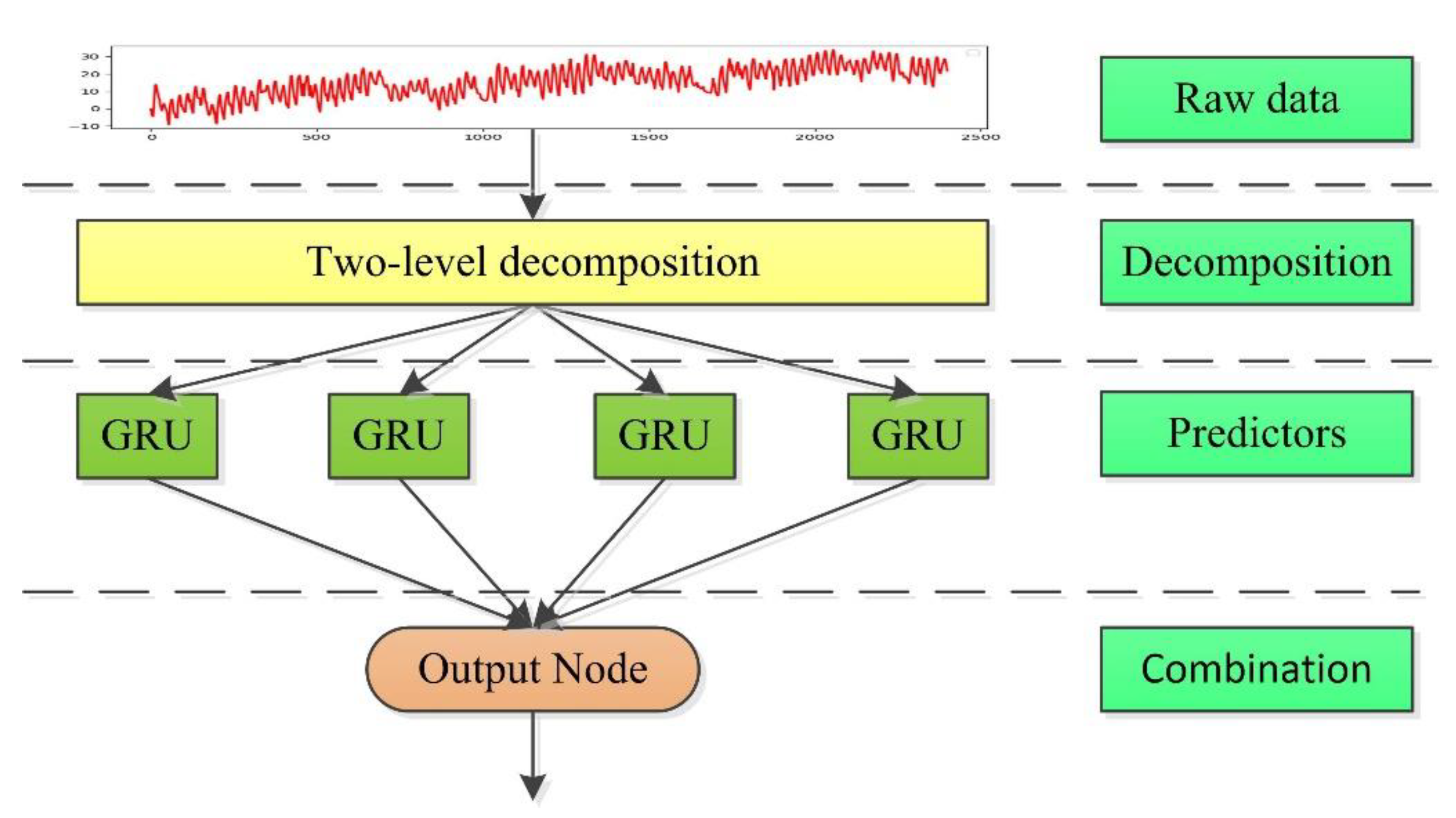
We present a general prediction framework for the IoT system that obtains accurate prediction of weather information, in which sub-predictors are designed based on four GRUs for the decomposed trend, periods, and residual components. Using the pick-up-data method, the input and output dimension was reduced to obtain long-term prediction for the following 30 days, and by expanding the prediction of the next day, the sub-prediction results were combined to obtain the accurate hourly prediction of temperature and humidity for the next day.

The rest of the paper is organized as follows. Section 2 discusses the research objective and introduces the data for experiments. The predictor is proposed in Section 3, especially the two-level decomposition and the prediction model structure. Section 3 gives the experiment results of the temperature and humidity data from the wolfberry plantation in Ningxia, China, and the results highlight applicability value of the proposed model. Finally, Section 4 summarizes and concludes the paper.

2. Research Objectives and Data Description

The IoT system was used for a wolfberry plantation in Ningxia province, China. Ningxia is one of the largest wolfberry planting areas in China. The area is a major crop for local farmers. At present, the planting area of Ningxia is 1 million mu, accounting for 33% of the total area of the whole country. The survival and growth of wolfberry plants are closely related to environmental factors such as temperature, humidity, etc. To understand and predict these weather factors is extremely important for the role and impact of precision cultivation of wolfberry.

According to future weather information, the planters can adjust the planting and picking plan, make full use of the advantages of local natural resources, and maintain the sustainable development of the planting industry.

Figure 2 shows the IoT system for precision agriculture. The IOT system is mainly composed of five parts: sensors, a display board, a computer, a controller, and an irrigation actuator. Because the planting is outdoor, we constructed an IoT system with a battery-powered wireless temperature and humidity sensor to collect the temperature and humidity data, being the data transmitted to the data center (a computer) for storage. Furthermore, a large quantity of stored data was used to train the deep learning model to give an accurate prediction of future temperature and humidity. The display board was mainly used to display the current weather conditions. The controller was used to control the irrigation actuator.

Based on the actual application needs, the requirements for the prediction results include the following two-terms prediction:

(1)

Medium-term prediction: Providing accurate predictions of temperature and humidity for the next 24 h;

(2)

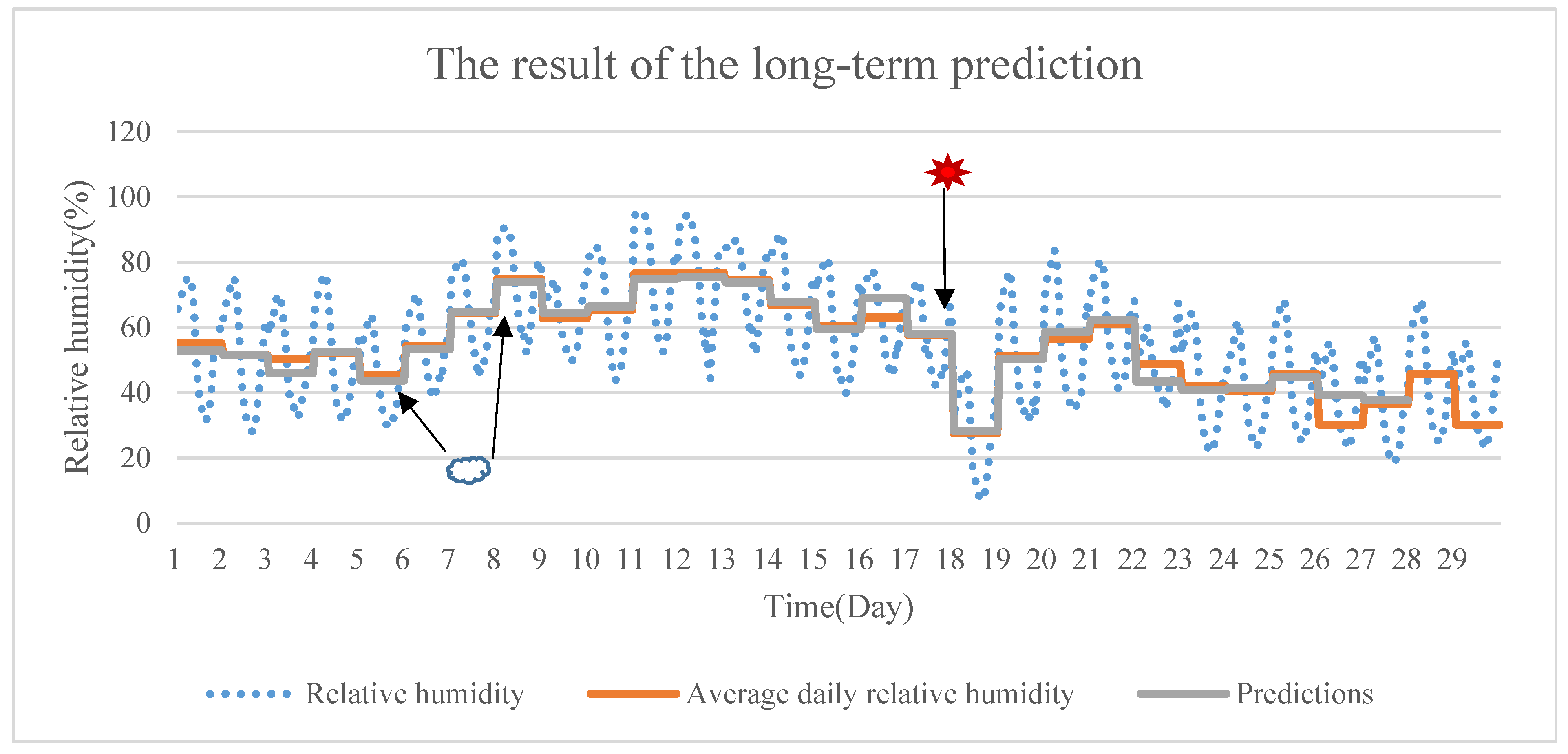
Long-term prediction: Providing average daily temperature and humidity for the next 30 days.

The former is used to guide the next day’s irrigation plan to ensure the effective use of water resources. Based on the accurate predictions of temperature and humidity in the next 24 h, the real-time irrigation time and irrigation volume are dynamically determined, and finally the automatic irrigation can be realized by using the irrigation control.

The latter is used to plan fertilization, harvesting, and picking, etc. Based on the accurate predictions of weather changes, these plans can improve agricultural sustainability.

To verify the prediction model, the temperature and humidity data were used with a total of 28,320 records from January 2016 to December 2017.

3. Distributed Decomposition Model

3.1. Model Framework

The model has three parts, i.e., decomposition, prediction, and combination. The prediction framework is shown in Figure 3. We used a two-level decomposition in which the original data were decomposed into four components. Then, each component was treated separately to obtain different GRU sub-predictors in the network training stage. In the prediction stage, different GRUs were used to predict the different components, respectively. Lastly, all the predictions were combined to get the final predicted results in the output node.

3.2. Sequential Two-Level Decomposition

A sequential two-level decomposition was used to decompose the raw time series data. The first-level decomposition period was 24 h and the trend, period per day, and residual were obtained. Because the residual obtained by the first-level decomposition still had periodicity, we used the second-level decomposition to decompose the residual into three further components.

Figure 4 shows the details of the decomposition node in Figure 3. By the first-level decomposition, the weather data, such as the temperature and humidity, were decomposed to the trend $T{D}_t$, the period per day $P{D}_t$ and the residual $R{D}_t$, and then the residual $R{D}_t$ was decomposed again, obtaining the trend $T{Y}_t$, the period per year $P{Y}_t$ and the residual $R{Y}_t$.

3.2.1. First-Level Decomposition

Assume that the time-sequential data $D_t$ has $N$ data, which means t = 1, 2, …, N. The relation with $Y_t$ and its three independent components, i.e., trend, period per day, and residual, is shown in Equation (1).

$$D_t=T{D}_t+P{D}_t+R{D}_t\hspace{1em}t=1,2,\dots ,N$$

(1)

where $T{D}_t$, $P{D}_t$, and $R{D}_t$ are trend component, period per day component, and residual component, respectively. The decomposition process is as follows:

(1)

Set the period for the first-level decomposition as 1 day, i.e., 24 h. For the data used in this study, that means 24 samples. Calculate the number of periods by $Num=\left[\frac{N}{24}\right]$, where $\left[a\right]$ is described to round up $a$.

(2)

Extract the trend $T{D}_t$ by the mean regression method to reflect the overall trend of the time series data.

(3)

Extract the period component of the data by the following two steps: $①$ Calculate $X{D}_t=D_t-T{D}_t$ to get the initial period component firstly. $②$ Select the data points from 1st to $Num\times 24$th in $X{D}_t$, add the data at the same time point, and then divide by $Num$ to obtain one period curve, and then copy it $Num$ times and consider the different of the $Num\times 24$ and $N$ to obtain the period component $P{D}_t$ with $N$ points.

(4)

Extract the residual component $R{D}_t$ by $R{D}_t=D_t-T{D}_t-P{D}_t$.

3.2.2. Second-Level Decomposition

We used a similar method for the second-level decomposition with the data as decomposed $R{D}_t$. Lastly, we obtained the mean value for each day. The relation with $R{D}_t$ and its three independent components, i.e., trend, period per year, and residual is the following.

$$R{D}_t=T{Y}_t+P{Y}_t+R{Y}_t\hspace{1em}t=1,2,\dots ,N$$

(2)

where $T{Y}_t$, $P{Y}_t$, and $R{Y}_t$ are the trend component, period component per year, and residual component, respectively. The decomposition process is as follows:

(1)

Set the period for the second-level decomposition as 1 year, i.e., $24\times 365=8760$ h. Then calculate the number of period components by $Num=\left[\frac{N}{8760}\right]$, where $\left[a\right]$ is described to round up $a$.

(2)

Extract the trend $T{Y}_t$ by the mean regression method to reflect the overall trend of the time series data.

(3)

Extract the period component of the data by the following two steps: $①$ Calculate $X{Y}_t=R{D}_t-T{Y}_t$ to get the initial period component firstly. $②$ Select the data points from 1st to $Num\times 8760$th in $X{Y}_t$, add the data at the same time point, and then divide by $Num$ to obtain one period curve and then copy it $Num$ times to obtain the component $XP{Y}_t$. $③$ Calculate the mean of each 24 h’ $XP{Y}_t$ to substitute the former point data, and obtain the period component $P{Y}_t$ with $N$ points.

(4)

Extract the residual component $R{Y}_t$ by $R{Y}_t=R{D}_t-T{Y}_t-P{Y}_t$.

3.3. Deep Learning Predictor

Two trends, i.e., $T{D}_t$ and $T{Y}_t$ were added as the trend component $T_t$. Considering this together with the other three components, i.e., the period per day $P{D}_t$ the period per year $P{Y}_t$ and the residual $R{Y}_t$, four components were used to train four GRU networks as the sub-predictors. Using the known input and output data, four GUR networks were trained by using supervised learning.

3.3.1. Sub-predictor GRU

The GRU network consists of multiple GRU cells. We set the number of layers as 2. Shown as Figure 5, $S_t$, $t=1,2,\dots ,n$ is the input of the GRU network, and $S_{t+n}$, $t=1,2,\dots ,n$ is the output.

The GRU uses the update gate to control the degree to which the state information of the previous moment is brought into the current state. The update gate and the reset gate were used to model the relation of input and output data. The forward propagation formulas in each GRU cell are as follows [29]:

$$\begin{array}{l}{z}_t=\sigma (a_t{U}^z+h_{t-1}{W}^z+b^z)\\ r_t=\sigma (a_t{U}^r+h_{t-1}{W}^r+b^r)\\ {\tilde{h}}_t=\tanh (a_t{U}^h+(h_{t-1}\circ r_t)W^h+b^h)\\ h_t=(1-z_t)\circ {\tilde{h}}_t+z_t\circ h_{t-1}\end{array}$$

(3)

where $a_t\in R^d$ is the input vector of each GRU cell; $z_t$, $r_t$, ${\tilde{h}}_t$, and $h_t$ stand for the update gate, reset gate, candidate state of the current hidden node, and the active state of the current hidden node output at time $t$, respectively; $U$ and $W$ are weight matrices to be learned during model training; $b$ represents bias vectors; $\circ$ is an element-wise multiplication; and $\sigma$ and $\tanh$ are activation functions.

In this research, we designed four GRUs as sub-predictors to predict four components, namely trend component $T_t$, the period per day $P{D}_t$, the period per year $P{Y}_t$ and the residual $R{Y}_t$. For long-term prediction, $S_t$ takes the component of the period per year $P{Y}_t$ and we set $n$ as 30. For medium-term prediction, $S_t$ takes the other three components and we set $n$ as 24. This means we used the data from the historical 24 h to predict the data of the future 24 h. The method proposed in this paper can be combined with other system identification methods [30,31,32] to study the modeling and prediction of other dynamic time series and random systems [33,34] and can be applied to other fields [35,36,37] and other signal modeling and control systems [6,38,39,40].

3.3.2. Long-term Prediction

As we mention in Section 2, long-term prediction provides the average daily temperature and humidity for the next 30 days. The period per year component of temperature and humidity of 30 days was used as the input and output data for training the GRU. The trend and residual components were used as compensation for the prediction.

We know from Section 3.2.2 that the period component per year $P{Y}_t$ is obtained by hourly data. Figure 6 gives an example of the period per year $P{Y}_t$ of 1 to 25, December 2017, with 648 hourly data. As a consequence, 30 days have 720 points. It is difficult to converge and train a network with 720 dimensions of input and output. Therefore, we picked up the average value of each day on the period component per year $P{Y}_t$ to construct the picked-up period per year $PP{Y}_t$.

By the picked-up period per year $PP{Y}_t$, the input and output data were reduced to 30. We organized the dataset for training by pushing back one step. The pushing process is shown in Figure 7, in which the data with the blue bars are input data, and the orange are output. Figure 7a shows the input data from 1st to 30th point and output data from the 31st to 60th point of $PP{Y}_t$ and Figure 7b is the input data from the 2nd to 31st, and output data from the 32nd to 61st point of $PP{Y}_t$.

Table 1. The input and output for training the GRU for long-term prediction.

	Input Data	Output Data
1	$PP{Y}_1$, $PP{Y}_2$, ……, $PP{Y}_{30}$	$PP{Y}_{31}$, $PP{Y}_{32}$, ……, $PP{Y}_{60}$
2	$PP{Y}_2$, $PP{Y}_3$, ……, $PP{Y}_{31}$	$PP{Y}_{32}$, $PP{Y}_{33}$, ……, $PP{Y}_{61}$
3	$PP{Y}_3$, $PP{Y}_4$, ……, $PP{Y}_{32}$	$PP{Y}_{33}$, $PP{Y}_{34}$, ……, $PP{Y}_{62}$
⋮	⋮	⋮
600	$PP{Y}_{601}$, $PP{Y}_{602}$, ……, $PP{Y}_{630}$	$PP{Y}_{631}$, $PP{Y}_{632}$, ……, $PP{Y}_{660}$

gives the 600 sets of input and output data used for training the sub-predictor GRU. The advantage of this overlapping input and output is that whenever new data are acquired, we can scroll forward based on the new data.

Once the parameters of sub-predictor GRU were obtained, by the test input data, the period per year could be predicted. By adding the mean of trend and residual component, we could obtain the long-term prediction with the average daily temperature and humidity of the next 30 days.

3.3.3. Medium-term Prediction

Medium-term prediction provides the accurate predictions of temperature and humidity for the next 24 h. The trend component $T_t$, the period per day $P{D}_t$ and the residual $R{Y}_t$ were used to train the other three GRUs to as the sub-predictors. The input and output data were set as 24 points.

The dataset for training was organized by pushing back 24 steps.

Table 2. The input and output for training the GRU with trend component $T_t$ for medium-term prediction.

	Input Data	Output Data
1	$T_1$, $T_2$, ……, $T_{24}$	$T_{25}$, $T_{26}$, ……, $T_{48}$
2	$T_{25}$, $T_{26}$, ……, $T_{48}$	$T_{49}$, $T_{50}$, ……, $T_{72}$
3	$T_{49}$, $T_{50}$, ……, $T_{72}$	$T_{73}$, $T_{74}$, ……, $T_{96}$
⋮	⋮	⋮
600	$T_{14377}$, $T_{14378}$, ……, $T_{14400}$	$T_{14401}$, $T_{14402}$, ……, $T_{14424}$

,

Table 3. The input and output for training the GRU with period per day component $P{D}_t$ for medium-term prediction.

	Input Data	Output Data
1	$P{D}_1$, $P{D}_2$, ……, $P{D}_{24}$	$P{D}_{25}$, $P{D}_{26}$, ……, $P{D}_{48}$
2	$P{D}_{25}$, $P{D}_{26}$, ……, $P{D}_{48}$	$P{D}_{49}$, $P{D}_{50}$, ……, $P{D}_{72}$
3	$P{D}_{49}$, $P{D}_{50}$, ……, $P{D}_{72}$	$P{D}_{73}$, $P{D}_{74}$, ……, $P{D}_{96}$
⋮	⋮	⋮
600	$P{D}_{14377}$, $P{D}_{14378}$, ……, $P{D}_{14400}$	$P{D}_{14401}$, $P{D}_{14402}$, ……, $P{D}_{14424}$

and

Table 4. The input and output for training the GRU with residual component $R{Y}_t$ for medium-term prediction.

	Input Data	Output Data
1	$R{Y}_1$, $R{Y}_2$, ……, $R{Y}_{24}$	$R{Y}_{25}$, $R{Y}_{26}$, ……, $R{Y}_{48}$
2	$R{Y}_{25}$, $R{Y}_{26}$, ……, $R{Y}_{48}$	$R{Y}_{49}$, $R{Y}_{50}$, ……, $R{Y}_{72}$
3	$R{Y}_{49}$, $R{Y}_{50}$, ……, $R{Y}_{72}$	$R{Y}_{73}$, $R{Y}_{74}$, ……, $R{Y}_{96}$
⋮	⋮	⋮
600	$R{Y}_{14377}$, $R{Y}_{14378}$, ……, $R{Y}_{14400}$	$R{Y}_{14401}$, $R{Y}_{14402}$, ……, $R{Y}_{14424}$

give the 600 sets of input and output data used for training.

With the training data shown in Table 2, Table 3 and Table 4, we could obtain three GRUs to predict the trend component $T_t$, the period per day $P{D}_t$ and the residual $R{Y}_t$ for the next 24 h. Based on the long-term prediction with average daily temperature for the next 30 days, we expended the next day’s value to 24 h’ average daily temperature (shown in Figure 8 in the top sub-figure with a yellow star). Then, the predictions were added, including trend component, daily mean value from the period per year, period per day, and residual for the next 24 h, to obtain the combined prediction.

4. Experiment Results and Discussion

4.1. Experimental Setup

The data used for training model were the collected hourly temperature and humidity data with about 35,040 records from January 2016 to December 2017. In the experiments, the ratio of the training set to the test set was 80:20.

The experiment hardware and software environments were set up to run the proposed prediction model. The open source deep learning library Keras, based on TensorFlow, was used to build all learning models. All experiments were performed on a PC with an Intel^® CORE™ CPU i5-4200U 1.60 GHz and 4 GB of memory. In order to model the deep neural network effectively, a large number of hyper parameters need to be set. In experiments, the default parameters in Keras were used for deep neural network initialization (e.g., weight initialization). We also used tanh as the activation function and ReLu as the activation function of the GRU model.

Usually, when we use neural networks to build models, the size of the network layer and the number of neurons is not strictly defined. Instead, the complexity of the model structure is determined based on the data. We determined the parameters of each layer of the model through multiple experimental adjustments. Specifically, we used the ReLu function. There were two GRU layers: the first layer had 30 neurons, and the second layer had 30 for predicting the picked-up period per year, and other GRUs had 24 neurons for these two layers (the number of neurons in the layers is determined by the output dimension of the model). In addition, all models underwent supervised training by using the Adam algorithm, which optimizes a predetermined objective function to obtain model parameters.

4.2. The Prediction Results

Figure 9 shows the long-term prediction of the temperature, in which the blue dotted line is the temperature data, the orange line is the average daily temperature, and the gray line is the predictions of the next 30 days. We can notice that at the first several days that the predictions are very close to the average daily temperature, while at the 10th day, the prediction is lower than the average daily temperature, and at the 15th and 23rd days, the prediction is higher than the average daily temperature. We can conclude that the long-term prediction can capture the rough changes of the future, while because the future weather is greatly affected by uncertain factors, it is impossible to accurately predict the effects of warm and cold air currents. There are similarities in the prediction of humidity (shown in Figure 10).

Because long-term forecasts are made every day, planting plans can change at any time if there is a sudden weather condition. The long-term prediction of weather information is used to designate rough planting plans for fertilization, harvesting, etc. for the next month, which is very beneficial for sustainable high-quality agricultural production.

Figure 11 and Figure 12 show the result of medium-term prediction. As an example, Figure 11 and Figure 12 show 4 days of predictions of the temperature and humidity, on December 1–4, 2017. The blue line is the temperature data and the orange line is the prediction result. We can find that these two lines are very close to each other, which indicates the obtained predictions are very accurate. Section 4.3 gives the numerical evaluation.

4.3. Comparing with Other Predictors

In this experiment, the proposed model was compared with eight other models, which are RNN [41], LSTM [42], BiLSTM [43], GRU [44], and the decomposition methods called seasonal-trend decomposition procedures based on loess (STL) [19] with RNN, LSTM, BiLSTM, and GRU as the sub-predictors, respectively. For evaluating the performance of the proposed predictor, root mean square error (RMSE) (shown in Equation (4)) is used as the evaluation metric to measure the difference between the prediction by a model and the collected data.

$$RMSE=\sqrt{\frac{{{\displaystyle {\sum }_{i=1}^N(x_{pre}(i)-x_{obs}(i))}}^2}{N}}$$

(4)

where $N$ is the number of prediction dataset; $x_{obs}$ represents the collected data; and $x_{pre}$ is predicted value.

The temperature and humidity data are used to show the prediction result.

Table 5. Comparison of root mean square error (RMSE) of prediction results with different predictors.

Model	RMSE of Temperature Predictions	RMSE of Relative Humidity Predictions
RNN	2.6682	14.0288
LSTM	2.9781	14.2898
BiLSTM	3.067	14.2683
GRU	3.0043	14.5584
STL_RNN	2.8155	13.8921
STL_LSTM	2.4940	13.6023
STL_BiLSTM	2.6482	14.0215
STL_GRU	2.5581	14.2546
The proposed model	2.4431	13.3041

gives a comparison of the predicted results of the RNN, LSTM, BiLSTM, GRU, STL_RNN (STL-based RNN), STL_LSTM (STL-based LSTM), STL_BiLSTM, STL_GRU, and two-level decomposition based on GRU (proposed in Section 3) models in terms of RMSE, and Figure 13 shows the histogram of RMSE. It is apparent from the comparison of prediction results that the decomposition models significantly outperform the undecomposed ones, and the proposed model has more accurate prediction than other models. For example, the prediction RMSE of the proposed model for temperature is approximately 20.34% and 2.04% lower, respectively, than that of the GRU and STL_LSTM models; for humidity, the RMSEs are about 8.61% and 2.19% lower, respectively. The results show that the developed two-level decomposition is effective because the RMSEs can be significantly reduced, and the GRU is the best choice as the sub-predictor.

5. Conclusions

In the precision agricultural IoT system, accurate prediction of weather data is a key way to improve the performance of the IoT system. The deep learning approach features self-learning capabilities and exhibits excellent performance in complex sensor data.

In this study, the two-level sequential decomposition structure was used to decompose the weather data according to different periods, thus reducing the complex nonlinear relationship of the raw data from sensors. By designing multiple GRUs as sub-predictors, the prediction results of sub-predictors were finally combined to obtain long-term and medium-term prediction of weather data. Through the verification of real data, the proposed model has higher prediction accuracy and can meet the needs of precision agriculture.

In precision agriculture, the use of the Internet of Things system can effectively reduce the workload of farmers and increase farmers’ awareness of the use of precision agricultural tools. According to our paper, long-term weather prediction can provide important guidance information for planning a reasonable growth cycle of crops. In addition, it can also help farmers manage farms. For example, there can be a preliminary forecast and estimation of severe weather in agriculture, so as to reduce risks and increase income.

References

1. Vecchio, Y.; Agnusdei, G.P.; Miglietta, P.P.; Capitanio, F. Adoption of Precision Farming Tools: The Case of Italian Farmers. Int. J. Environ. Res. Public Health 2020, 17, 869. [Google Scholar] [CrossRef] [Green Version]
2. Fusco, G.; Miglietta, P.P.; Porrini, D. How Drought Affects Agricultural Insurance Policies: The Case of Italy. J. Sustain. Dev. 2018, 1111, 1–13. [Google Scholar] [CrossRef]
3. Porrini, D.; Fusco, G.; Miglietta, P.P. Post-adversities recovery and profitability: The case of Italian farmers. Int. J. Environ. Res. Public Health 2019, 16, 3189. [Google Scholar] [CrossRef] [Green Version]
4. Muangprathub, J.; Boonnam, N.; Kajornkasirat, S.; Lekbangpong, N.; Wanichsombat, A.; Nillaor, P. IoT and agriculture data analysis for smart farm. Comput. Electron. Agric. 2019, 156, 467–474. [Google Scholar] [CrossRef]
5. Suciu, G.; Marcu, I.; Balaceanu, C.; Dobrea, M.; Botezat, E. Efficient IoT System for Precision Agriculture. In Proceedings of the 2019 15th International Conference on Engineering of Modern Electric Systems (EMES), Oradea, Romania, 13–14 June 2019; Volume 13–14, pp. 173–176. [Google Scholar]
6. Zhao, Z.; Yao, P.; Wang, X.; Xu, J.; Wang, L.; Yu, J. Reliable flight performance assessment of multirotor based on interacting multiple model particle filter and health degree. Chin. J. Aeronaut. 2019, 32, 444–453. [Google Scholar] [CrossRef]
7. Keswani, B.; Mohapatra, A.G.; Mohanty, A.; Khanna, A.; Rodrigues, J.J.P.C.; Gupta, D.; Albuquerque, V.H.C. Adapting weather conditions based IoT enabled smart irrigation technique in precision agriculture mechanisms. Neural Comput. Appl. 2019, 3131, 277–292. [Google Scholar] [CrossRef]
8. Mohammadi, M.; Al-Fuqaha, A.; Sorour, S.; Guizani, M. Deep learning for IoT big data and streaming analytics: A survey. IEEE Commun. Surv. Tutor. 2018, 20, 2923–2960. [Google Scholar] [CrossRef] [Green Version]
9. Bai, Y.T.; Jin, X.B.; Wang, X.Y.; Wang, X.K.; Xu, J.P. Dynamic correlation analysis method of air pollutants in spatio-temporal analysis. Int. J. Environ. Res. Public Health 2020, 17, 360. [Google Scholar] [CrossRef] [PubMed] [Green Version]
10. Benmouiza, K.; Cheknane, A. Small-scale solar radiation forecasting using ARMA and nonlinear autoregressive neural network models. Theor. Appl. Climatol. 2016, 124, 945–958. [Google Scholar] [CrossRef]
11. Wang, L.; Zhang, T.; Jin, X.; Xu, J.; Wang, X.; Zhang, H.; Yu, J.; Sun, Q.; Zhao, Z.; Xie, Y. An approach of recursive timing deep belief network for algal bloom forecasting. Neural Comput. Appl. 2020, 32, 163–171. [Google Scholar] [CrossRef]
12. Bai, Y.; Jin, X.; Wang, X.; Su, T.; Kong, J.; Lu, Y. Compound autoregressive network for prediction of multivariate time series. Complexity 2019, 2019, 9107167. [Google Scholar] [CrossRef]
13. Wang, L.; Zhang, T.; Wang, X.; Jin, X.; Xu, J.; Yu, J.; Zhang, H.; Zhao, Z. An approach of improved Multivariate Timing-Random Deep Belief Net modelling for algal bloom prediction. Neural Comput. Appl. 2019, 177, 130–138. [Google Scholar] [CrossRef]
14. Mao, J.D.; Zhang, X.J.; Li, J. Wind Power Forecasting Based on the BP Neural Network. Appl. Mech. Mater. 2013, 341–342, 1303–1307. [Google Scholar] [CrossRef] [Green Version]
15. Smits, G.F.; Jordaan, E.M. Improved SVM Regression Using Mixtures of Kernels. In Proceedings of the 2002 International Joint Conference on Neural Networks, Honolulu, HI, USA, 12–17 May 2002; IEEE: Piscataway, NJ, USA; Volume 3, pp. 2785–2790. [Google Scholar]
16. Xu, X.; Ren, W. Application of a Hybrid Model Based on Echo State Network and Improved Particle Swarm Optimization in PM2. 5 Concentration Forecasting: A Case Study of Beijing, China. Sustainability 2019, 11, 3096. [Google Scholar] [CrossRef] [Green Version]
17. Zheng, Y.Y.; Kong, J.L.; Jin, X.B.; Wang, X.Y.; Su, T.L.; Zuo, M. Cropdeep: The crop vision dataset for deep-learning-based classification and detection in precision agriculture. Sensors 2019, 19, 1058. [Google Scholar] [CrossRef] [PubMed] [Green Version]
18. Xu, J.; Rahmatizadeh, R.; Boloni, L.; Bölöni, L.; Turgut, D. Real-Time Prediction of Taxi Demand Using Recurrent Neural Networks. IEEE Trans. Intell. Transp. Syst. 2017, 19, 2572–2581. [Google Scholar] [CrossRef]
19. Sakar, C.O.; Polat, S.O.; Katircioglu, M.; Kastro, Y. Real-time prediction of online shoppers’ purchasing intention using multilayer perceptron and LSTM recurrent neural networks. Neural Comput. Appl. 2019, 31, 6893–6908. [Google Scholar] [CrossRef]
20. Che, Z.; Purushotham, S.; Cho, K.; Sontag, D.; Liu, Y. Recurrent Neural Networks for Multivariate Time Series with Missing Values. Sci. Rep. 2018, 8, 6085. [Google Scholar] [CrossRef] [Green Version]
21. Yao, Y.; Huang, Z. Bi-directional LSTM Recurrent Neural Network for Chinese Word Segmentation. In Lecture Notes in Computer Science, Proceedings of the ICONIP 2016 Neural Information Processing, Kyoto, Japan, 16–21 October 2016; Hirose, A., Ozawa, S., Doya, K., Ikeda, K., Lee, M., Liu, D., Eds.; Springer: Cham, Switzerland, 2016; Volume 9950. [Google Scholar]
22. Tang, Y.; Huang, Y.; Wu, Z.; Meng, H.; Xu, M.X.; Cai, L.H. Question Detection from Acoustic Features Using Recurrent Neural Network with Gated Recurrent Unit. In Proceedings of the 2016 IEEE International Conference on Acoustics, Speech and Signal Processing (ICASSP), Shanghai, China, 19 May 2016; IEEE: Piscataway, NJ, USA. [Google Scholar]
23. Chung, J.; Gulcehre, C.; Cho, K.H.; Bengio, Y. Empirical evaluation of gated recurrent neural networks on sequence modeling. arXiv 2014, arXiv:1412.3555. [Google Scholar]
24. Jin, X.; Yang, N.; Wang, X.; Bai, Y.; Su, T.; Kong, J. Integrated predictor based on decomposition mechanism for PM2. 5 long-term prediction. Appl. Sci. 2019, 9, 4533. [Google Scholar] [CrossRef] [Green Version]
25. García-Mozo, H.; Oteros, J.A.; Galán, C. Impact of land cover changes and climate on the main airborne pollen types in Southern Spain. Sci. Total Environ. 2016, 548, 221–228. [Google Scholar] [CrossRef] [PubMed]
26. Rojo, J.; Rivero, R.; Romero-Morte, J.; Fernández-González, F.; Pérez-Badia, R. Modeling pollen time series using seasonal-trend decomposition procedure based on LOESS smoothing. Int. J. Biometeorol. 2017, 61, 335–348. [Google Scholar] [CrossRef] [PubMed]
27. Ming, F.; Yang, Y.X.; Zeng, A.M.; Jing, Y.F. Analysis of seasonal signals and long-term trends in the height time series of IGS sites in China. Sci. China Earth Sci. 2016, 59, 1283–1291. [Google Scholar] [CrossRef]
28. Qin, L.; Li, W.; Li, S. Effective passenger flow forecasting using STL and ESN based on two improvement strategies. Neurocomputing 2019, 356, 244–256. [Google Scholar] [CrossRef]
29. Yang, W.; Zuo, W.; Cui, B. Detecting malicious urls via a keyword-based convolutional gated-recurrent-unit neural network. IEEE Access 2019, 7, 29891–29900. [Google Scholar] [CrossRef]
30. Ding, F.; Xu, L.; Meng, D.; Jin, X.-B.; Alsaedi, A.; Hayat, T. Gradient estimation algorithms for the parameter identification of bilinear systems using the auxiliary model. J. Comput. Appl. Math. 2020, 369, 112575. [Google Scholar] [CrossRef]
31. Cui, T.; Ding, F.; Jin, X.; Alsaedi, A.; Hayat, T. Joint Multi-innovation Recursive Extended Least Squares Parameter and State Estimation for a Class of State-space Systems. Int. J. Control Autom. Syst. 2020, 18, 1–13. [Google Scholar] [CrossRef]
32. Ding, F.; Lv, L.; Pan, J.; Wan, X.; Jin, X.-B. Two-stage Gradient-based Iterative Estimation Methods for Controlled Autoregressive Systems Using the Measurement Data. Int. J. Control Autom. Syst. 2020, 18, 1–11. [Google Scholar] [CrossRef]
33. Wang, X.; Zhou, Y.; Zhao, Z.; Wang, L.; Xu, J.; Yu, J. A novel water quality mechanism modeling and eutrophication risk assessment method of lakes and reservoirs. Nonlinear Dyn. 2019, 96, 1037–1053. [Google Scholar] [CrossRef]
34. Yu, J.; Deng, W.; Zhao, Z.; Wang, X.; Xu, J.; Wang, L.; Sun, Q.; Shen, Z. A hybrid path planning method for an unmanned cruise ship in water quality sampling. IEEE Access 2019, 7, 87127–87140. [Google Scholar] [CrossRef]
35. Wang, F.; Su, T.; Jin, X.; Zheng, Y.; Kong, J.; Bai, Y. Indoor Tracking by RFID Fusion with IMU Data. Asian J. Control 2019, 21, 1768–1777. [Google Scholar] [CrossRef]
36. Wang, Z.; Jin, X.; Wang, X.; Xu, J.; Bai, Y. Hard decision-based cooperative localization for wireless sensor networks. Sensors 2019, 19, 4665. [Google Scholar] [CrossRef] [PubMed] [Green Version]
37. Jin, X.; Yang, N.; Wang, X.; Bai, Y.; Su, T.; Kong, J. Deep Hybrid Model Based on EMD with Classification by Frequency Characteristics for Long-Term Air Quality Prediction. Mathematics 2020, 8, 214. [Google Scholar] [CrossRef] [Green Version]
38. Wang, X.; Zhou, Y.; Zhao, Z.; Wei, W.; Li, W. Time-Delay System Control Based on an Integration of Active Disturbance Rejection and Modified Twice Optimal Control. IEEE Access 2019, 7, 130734–130744. [Google Scholar] [CrossRef]
39. Bai., Y.; Wang, X.; Jin, X. Adaptive filtering for MEMS gyroscope with dynamic noise model. ISA Trans. 2020. [Google Scholar] [CrossRef]
40. Bai, Y.; Wang, X.; Jin, X.; Zhao, Z.; Zhang, B. A neuron-based kalman filter with nonlinear autoregressive model. Sensors 2020, 20, 299. [Google Scholar] [CrossRef] [Green Version]
41. Zhang, J.S.; Xiao, X.C. Predicting chaotic time series using recurrent neural network. Chin. Phys. Lett. 2000, 17, 88. [Google Scholar] [CrossRef]
42. Gers, F.A.; Schraudolph, N.N.; Schmidhuber, J. Learning precise timing with LSTM recurrent networks. J. Mach. Learn. Res. 2002, 3, 115–143. [Google Scholar]
43. Kiperwasser, E.; Goldberg, Y. Simple and accurate dependency parsing using bidirectional LSTM feature representations. Trans. Assoc. Comput. Linguist. 2016, 4, 313–327. [Google Scholar] [CrossRef]
44. Shen, G.; Tan, Q.; Zhang, H.; Zeng, P.; Xu, J. Deep learning with gated recurrent unit networks for financial sequence predictions. Procedia Comput. Sci. 2018, 131, 895–903. [Google Scholar] [CrossRef]
Figure 1. Decomposition of temperature data in Ningxia, China.
Sustainability 12 01433 g001
Figure 2. Data collection and prediction in the IoT system for precision agriculture.
Sustainability 12 01433 g002
Figure 3. Flowchart of prediction framework.
Sustainability 12 01433 g003
Figure 4. The structure of sequential two-level decomposition.
Sustainability 12 01433 g004
Figure 5. Network structure of the gated recurrent unit (GRU).
Sustainability 12 01433 g005
Figure 6. An example of the period per year P Y t and picked-up period per year P P Y t .
Sustainability 12 01433 g006
Figure 7. The input and output data for training the GRU by pushing back one step.
Sustainability 12 01433 g007aSustainability 12 01433 g007b
Figure 8. Schematic diagram of medium-term prediction.
Sustainability 12 01433 g008
Figure 9. The temperature result of long-term prediction.
Sustainability 12 01433 g009
Figure 10. The humidity result of long-term prediction.
Sustainability 12 01433 g010
Figure 11. The temperature result of medium-term prediction.
Sustainability 12 01433 g011
Figure 12. The humidity result of medium-term prediction.
Sustainability 12 01433 g012
Figure 13. The histogram of RMSE for prediction of temperature and humidity.
Sustainability 12 01433 g013