Analysis of Problems Related to the Calculation of Flood Frequency Using Rainfall-Runoff Models: A Case Study in Poland


Abstract
:1. Introduction
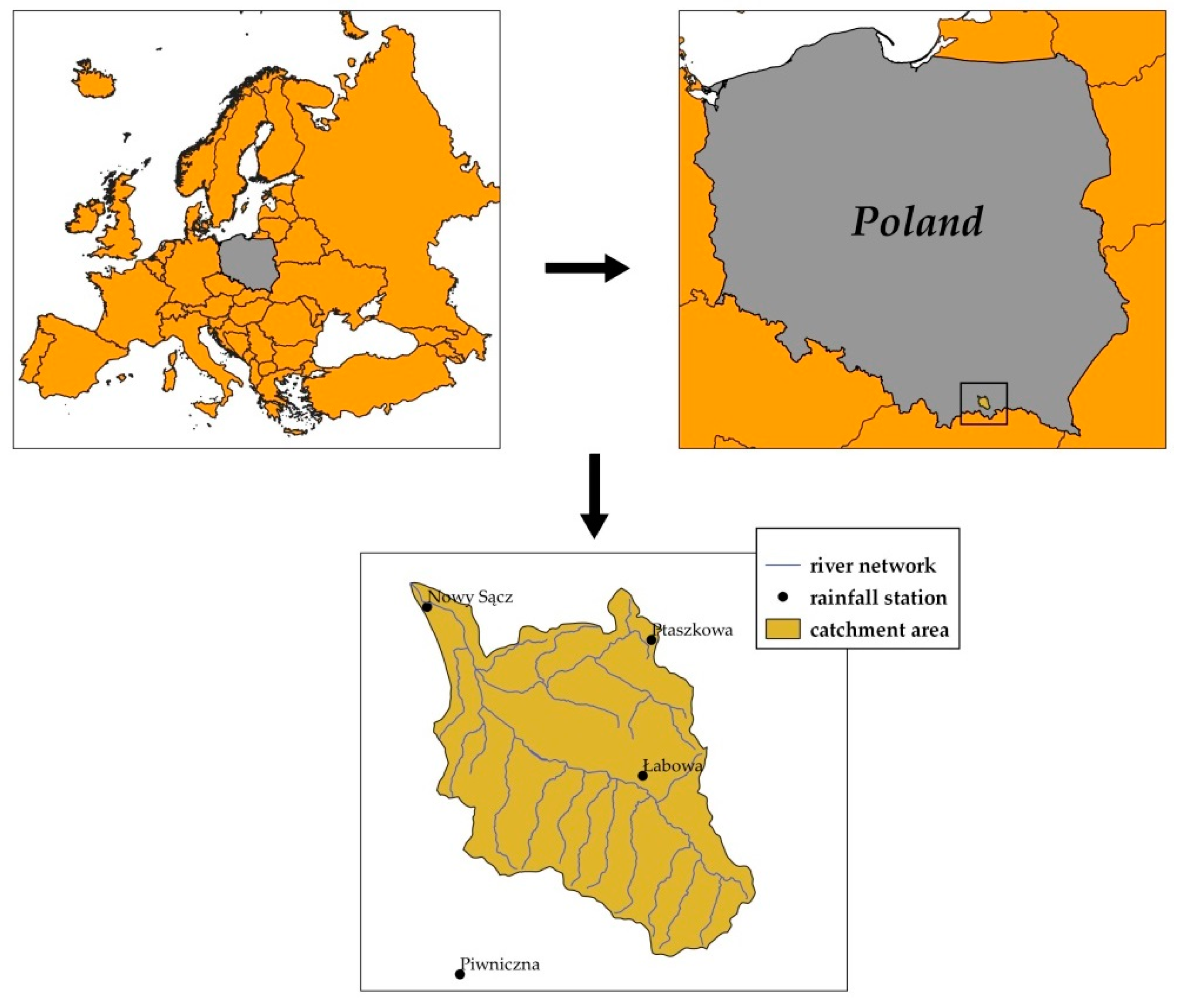
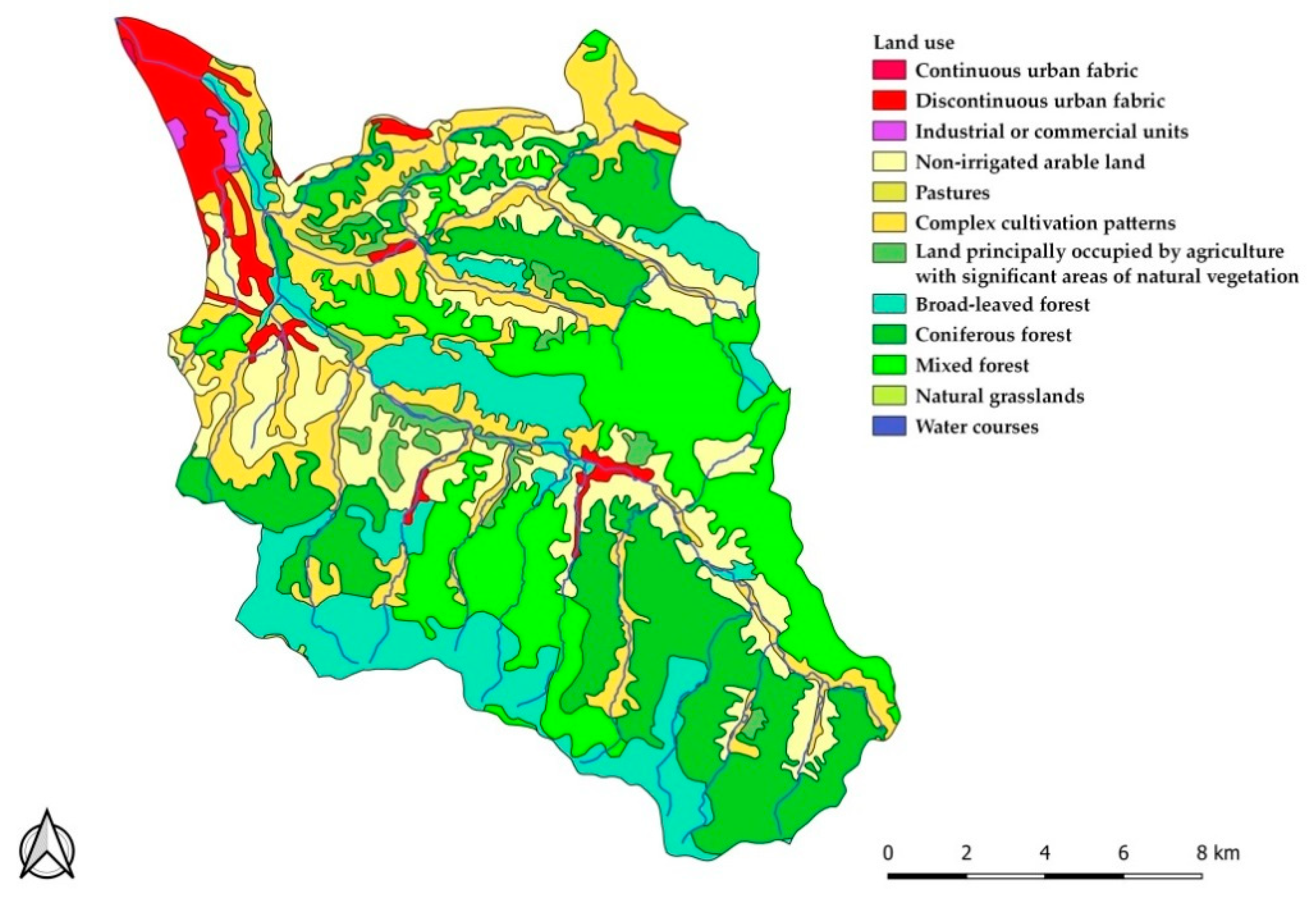
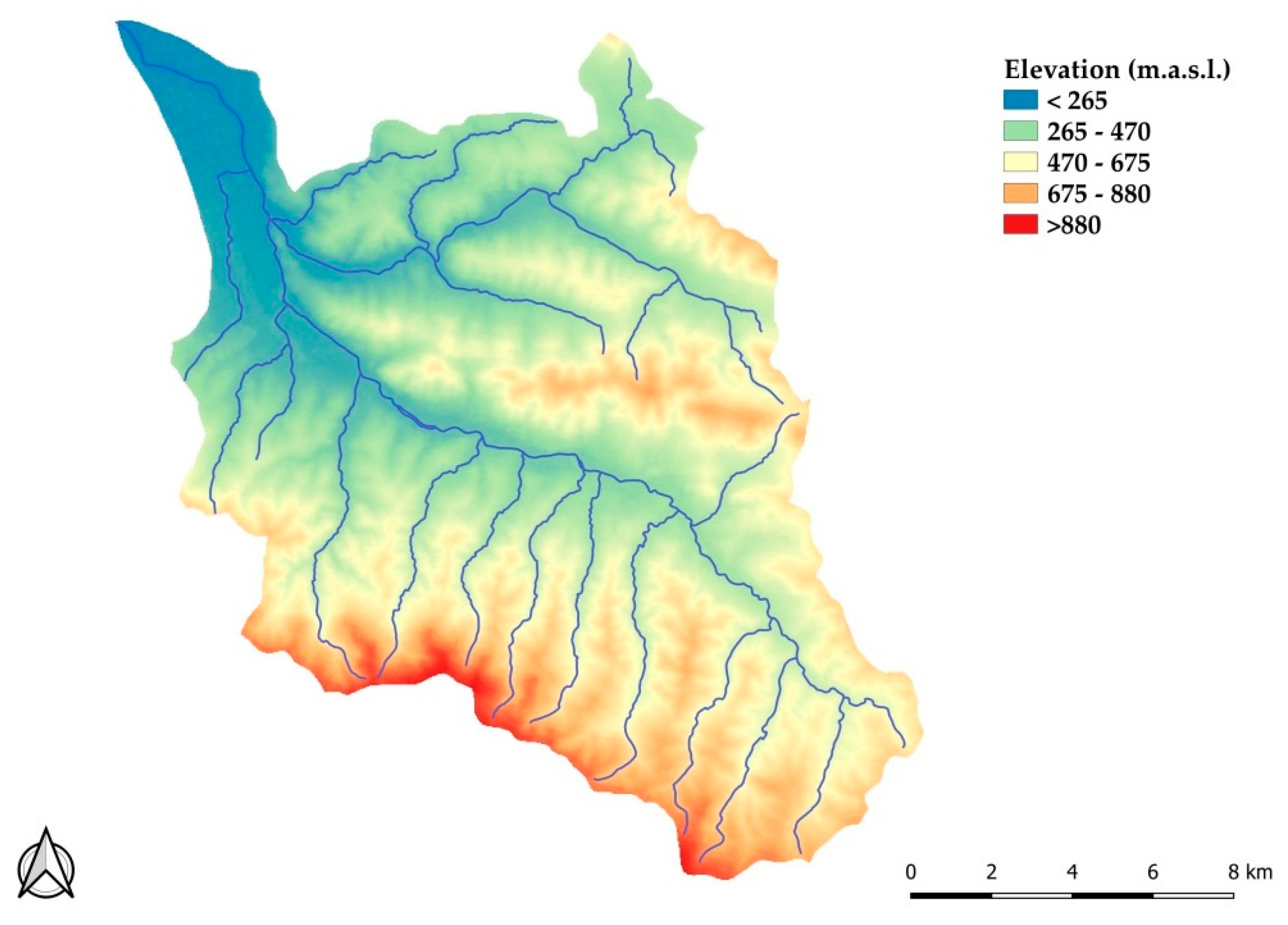
2. Study Area
3. Materials and Methods
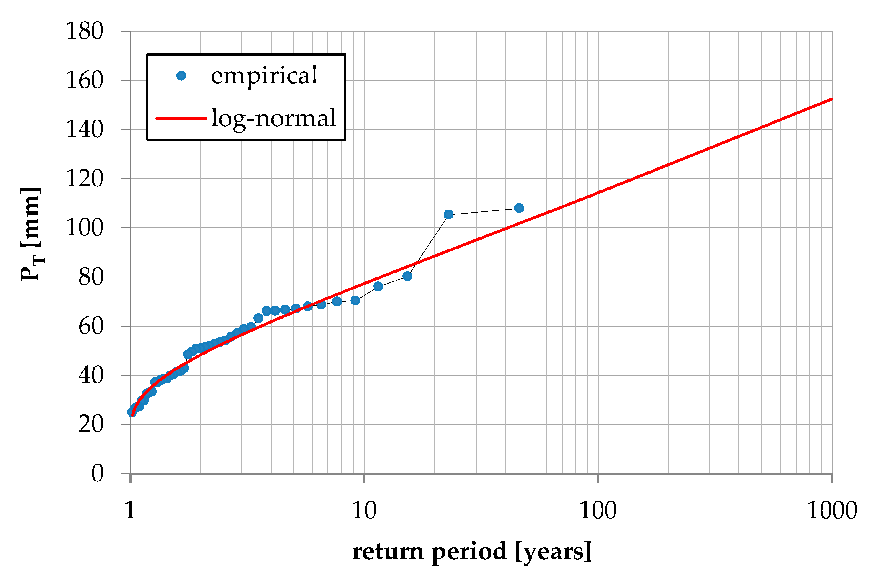
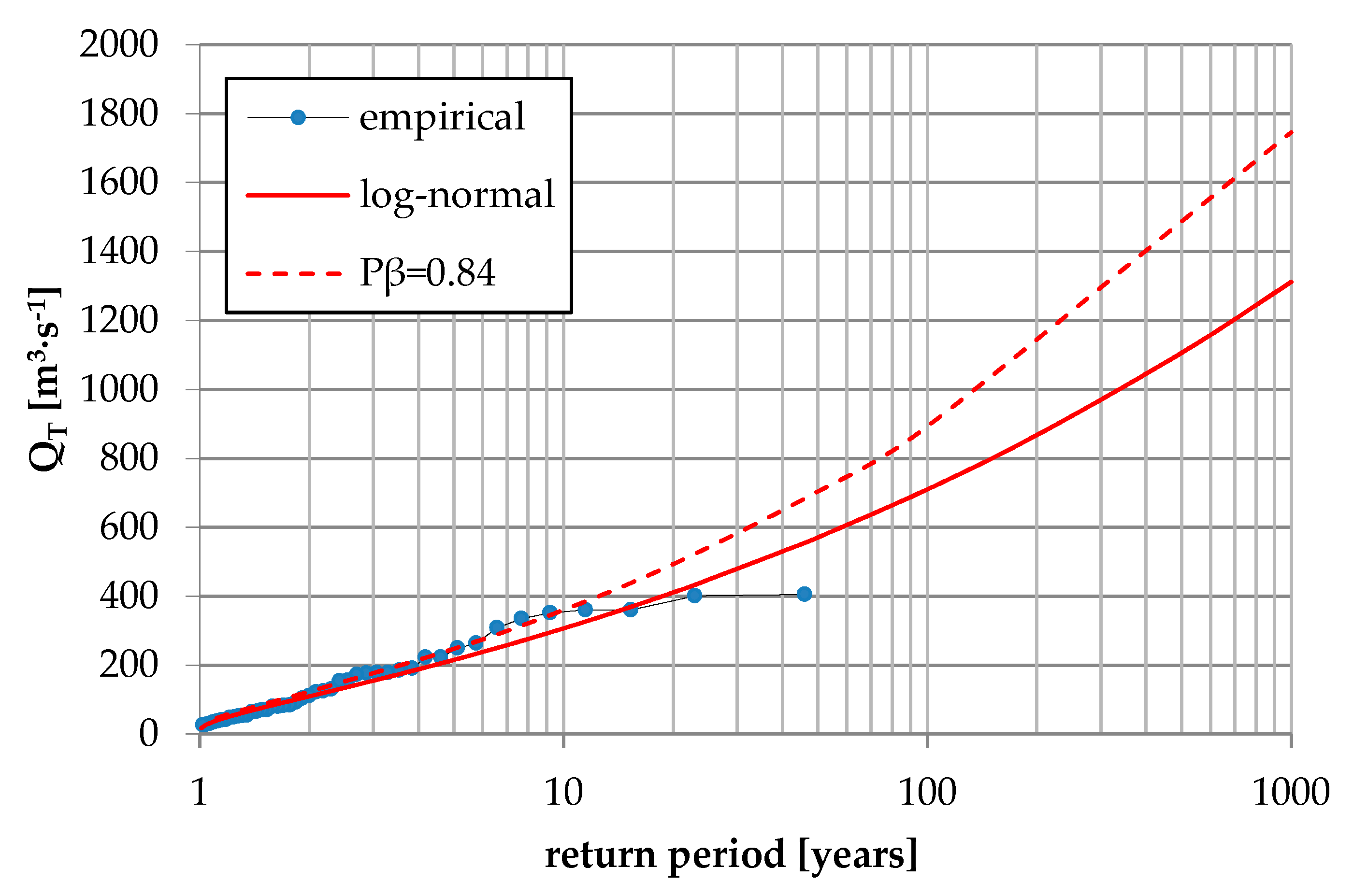
3.1. Determination of Design Precipitation and Design Flows Using Statistical Method
- xp—quantile of the theoretical log-normal distribution;
- ε—lower string limit,
- erf(2(1 − p) − 1)—Gauss error function.
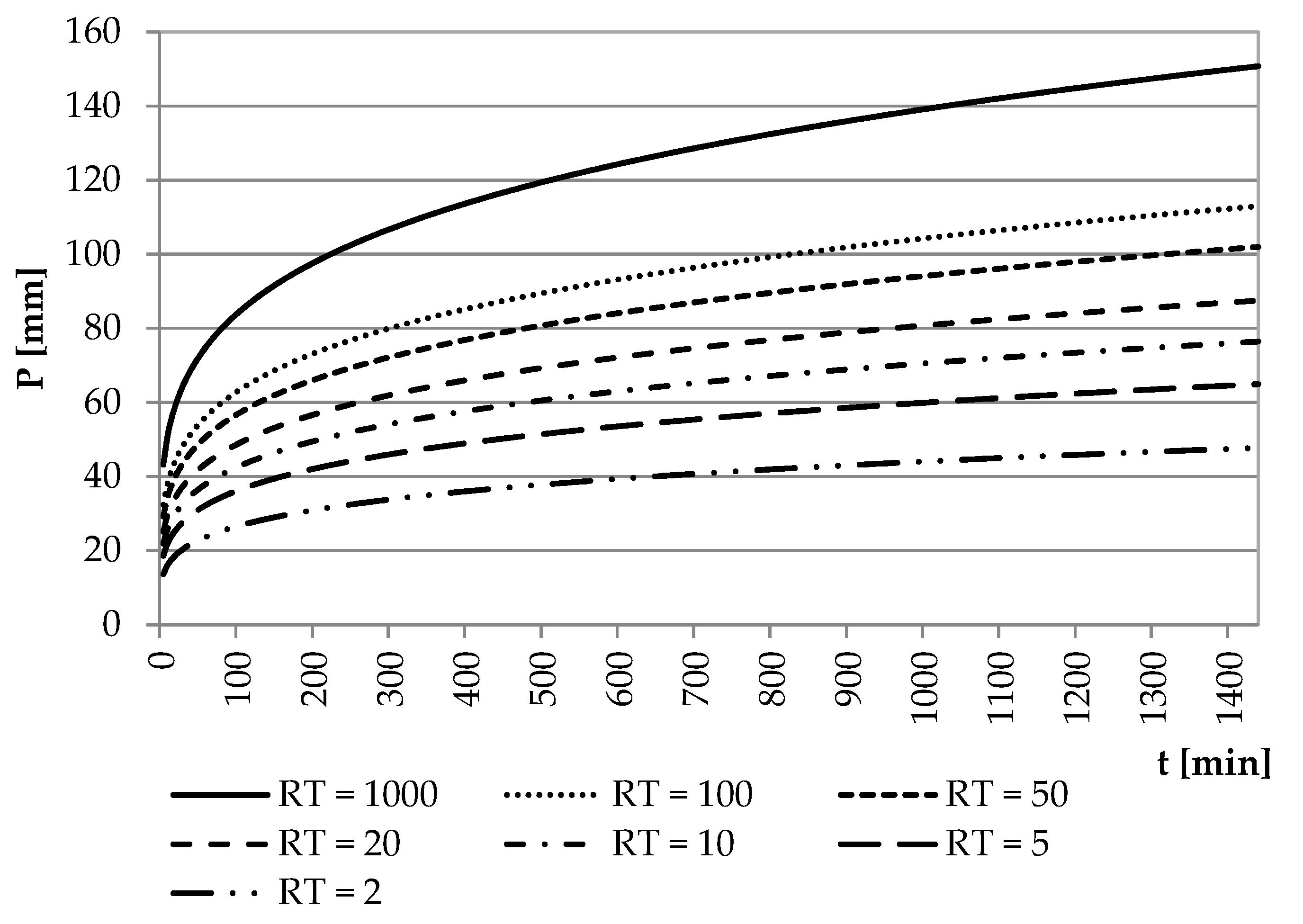
- Ψ(t)—precipitation reduction factor (-),
- t—duration of precipitation (min),
- P(Tc)—precipitation for a time equal to the concentration time (mm),
- PT—design precipitation with the same return period (mm),
- Tc—concentration time (min).
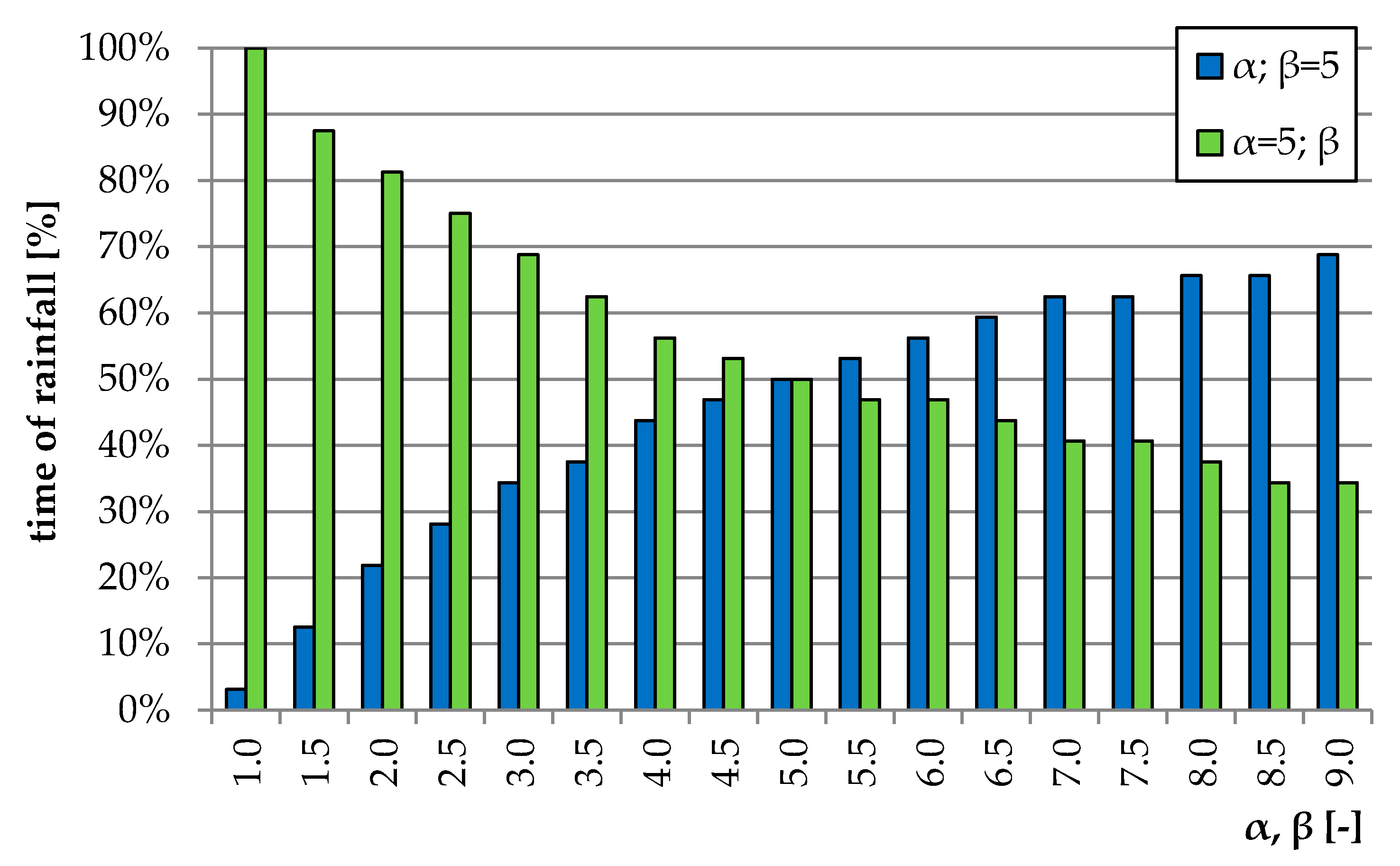
3.2. Determination of the Design Hyetograph
- α, β—shape factors (α > 0, β > 0),
- B—value of the beta function,
- t—duration of precipitation.
3.3. Determination of Design Flows Using the Snyder Model
- Pe—excessive rainfall [mm],
- P—total rainfall [mm],
- S—maximum potential catchment retention [mm].
- TL—delay time [h],
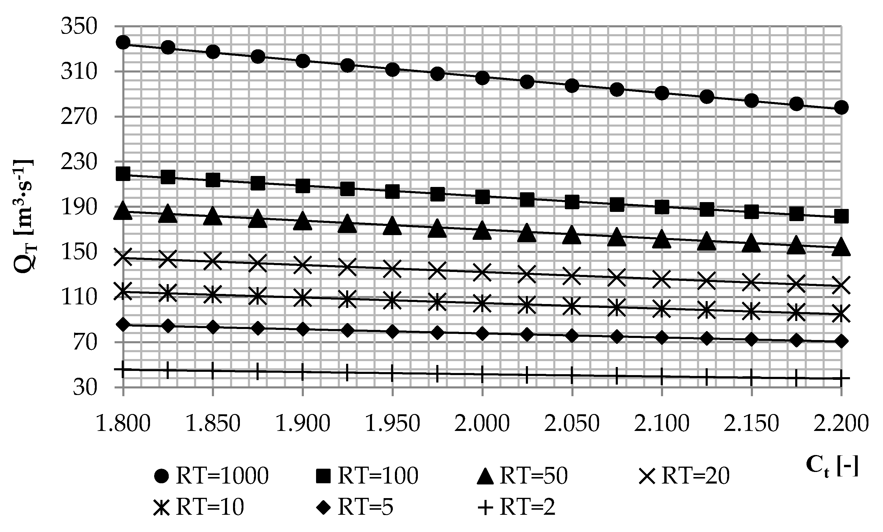
- Ct—coefficient related to the catchment retention range from 1.8 to 2.2 [-],
- L—distance along the watercourse from the closing cross-section to the intersection of the dry valley with the watershed [km],
- Lc—distance along the main watercourse from the mouth section to the center of gravity of the catchment area [km].
- Qp—peak flow of unit hydrograph [m3·s−1·mm],
- Cp—empirical coefficient resulting from the simplification of the hydrograph to triangle, taking values from 0.4 to 0.8 [-],
- A—catchment area [km2].
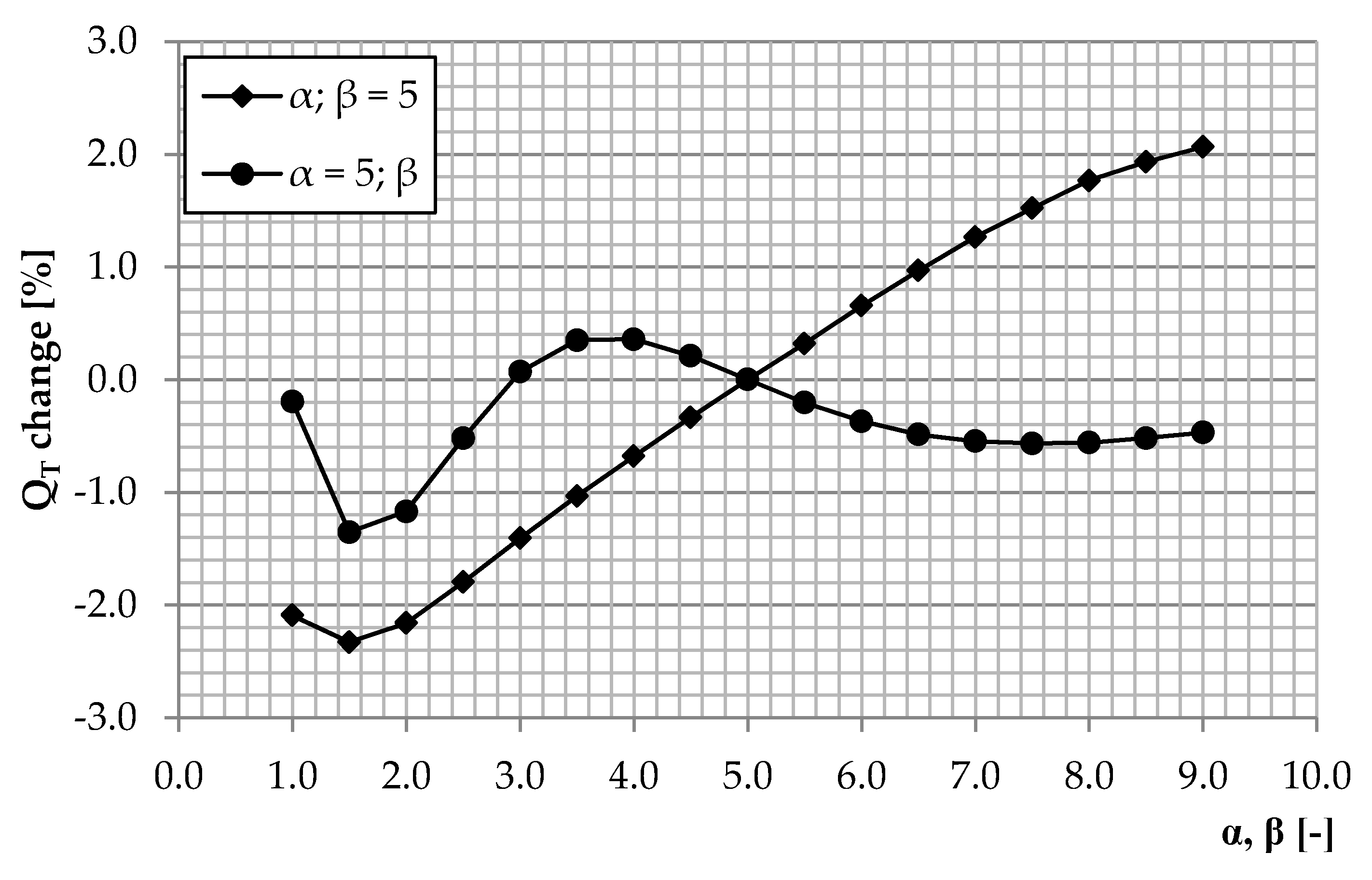
3.4. Evaluation of the Quality of Work of the Snyder Model
- QT—maximum flow with a given frequency of occurrence, calculated using the log-normal distribution [m3·s−1],
- —maximum flow with a given occurrence frequency, calculated using the Snyder model [m3·s−1].
4. Results and Discussion
4.1. Determination of Design Precipitation and Flows
4.2. Determination of Precipitation Hyetograph
4.3. Determining the Value of Design Flows Using the Snyder Model
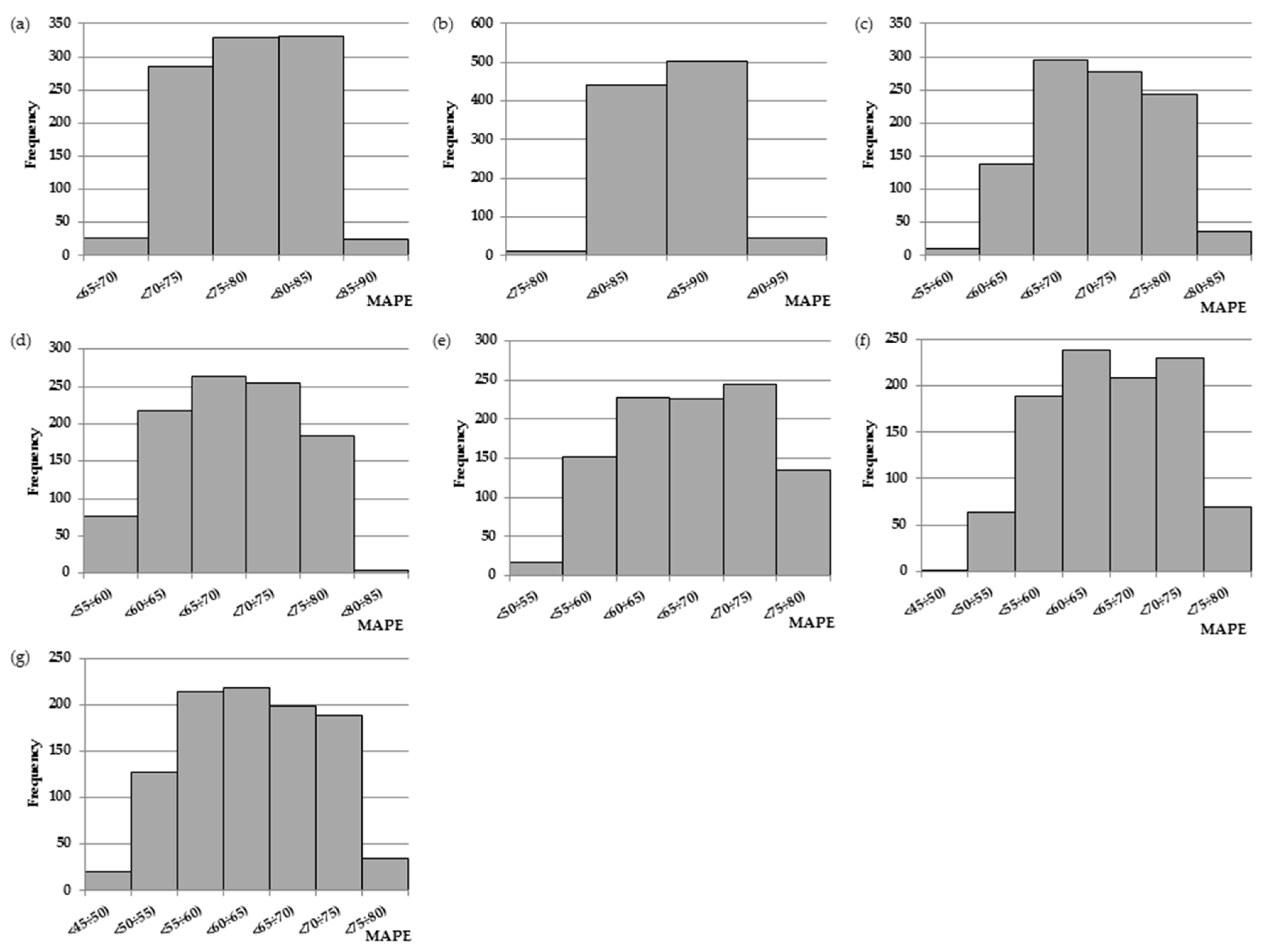
4.4. Determining Relative Error
5. Conclusions
Funding
Acknowledgments
Conflicts of Interest
References
- Karabová, B.; Sikorska-Senoener, A.E.; Banasik, K.; Kohnová, S. Rainfallrunoff model for a small catchment in Carpathians. Ann. Warsaw Univ. Life Sci. SGGW. Land Reclam. 2012, 44, 155–162. [Google Scholar] [CrossRef]
- Vaššová, D. Comparison of rainfall-runoff models for design discharge assessment in a small ungauged catchment. Soil Water Res. 2013, 8, 26–33. [Google Scholar] [CrossRef] [Green Version]
- Khaleghi, M.R.; Ghodusi, J.; Ahmadi, H. Regional analysis using the Geomorphologic Instantaneous Unit Hydrograph (GIUH) method. Soil Water Res. 2014, 9, 25–30. [Google Scholar] [CrossRef] [Green Version]
- Jena, J.; Nath, S. An empirical formula for design flood estimation of un-gauged catchments in Brahmani Basin, Odisha. J. Inst. Eng. India Ser. A 2020, 101, 1–6. [Google Scholar] [CrossRef]
- Hrachowitz, M.; Savenije, H.H.G.; Blöschl, G.; McDonnell, J.J.; Sivapalan, M.; Pomeroy, J.W.; Arheimer, B.; Blume, T.; Clark, M.P.; Ehret, U.; et al. A decade of Predictions in Ungauged Basins (PUB)—A review. Hydrol. Sci. J. 2013, 58, 1198–1255. [Google Scholar] [CrossRef]
- Dhakal, N.; Fang, X.; Asquith, W.H.; Cleveland, T.G.; Thompson, D.B. Return period adjustment for runoff coefficients based on analysis in undeveloped Texas watersheds. J. Irrig. Drain. Eng. ASCE 2013, 139, 476–482. [Google Scholar] [CrossRef] [Green Version]
- Piscopia, R.; Petroselli, A.; Grimaldi, S. A software package for the prediction of design flood hydrograph in small and ungauged basins. J. Agric. Eng. 2015, 432, 74–84. [Google Scholar]
- Petroselli, A.; Grimaldi, S. Design hydrograph estimation in small and fully ungauged basin: A preliminary assessment of the EBA4SUB framework. J. Flood Risk Manag. 2018, 11, 197–2010. [Google Scholar] [CrossRef]
- Salami, A.W.; Bilewu, S.O.; Ibitoye, A.B.; Ayanshola, A.M. Runoff hydrographs using Snyder and SCS unit hydrograph methods: A case study of selected rivers in south west Nigeria. J. Ecol. Eng. 2017, 18, 25–34. [Google Scholar] [CrossRef] [Green Version]
- Federova, D.; Kovář, P.; Gregar, J.; Jelínková, A.; Novotná, J. The use of Snyder synthetic hydrograph for simulation of overland flow in small ungauged and gauged catchments. Soil Water Res. 2018, 13, 185–192. [Google Scholar]
- Blair, A.; Sanger, D.; White, D.; Holland, A.F.; Vandiver, L.; Bowker, C.; White, S. Quantifying and simulating stormwater runoff in watersheds. Hydrol. Process. 2012, 28, 559–569. [Google Scholar] [CrossRef]
- Banasik, K.; Rutkowska, A.; Kohnová, S. Retention and Curve Number variability in a small agricultural catchment: The probabilistic approach. Water 2014, 6, 1118–1133. [Google Scholar] [CrossRef]
- Kowalik, T.; Wałęga, A. Estimation of CN Parameter for small agricultural watersheds using asymptotic functions. Water 2015, 7, 939–955. [Google Scholar] [CrossRef] [Green Version]
- Wałega, A.; Książek, L. Influence of rainfall data on the uncertainty of flood simulation. Soil Water Res. 2016, 11, 277–284. [Google Scholar] [CrossRef] [Green Version]
- Wałęga, A. The importance of calibration parameters on the accuracy of the floods description in the Snyder’s model. J. Water Land Dev. 2016, 28, 19–25. [Google Scholar] [CrossRef]
- Chen, F.W.; Liu, C.W. Estimation of the spatial rainfall distribution using inverse distance weighting (IDW) in the middle of Taiwan. Paddy Water Environ. 2012, 10, 209–222. [Google Scholar] [CrossRef]
- Viglione, A.; Blöschl, G. On the role of storm duration in the mapping of rainfall to flood return period. Hydrol. Earth Syst. Sci. Discuss. 2008, 5, 3419–3447. [Google Scholar] [CrossRef]
- Hogg, R.V.; Craig, A.T. Introduction to Mathematical Statistics; Macmilan Publishing Co.: New York, NY, USA, 1978. [Google Scholar]
- Petroselli, A.; Vojtek, M.; Vojteková, J. Flood mapping in small ungauged basins: A comparisonof different approaches for two case studies in Slovakia. Hydrol. Res. 2019, 50, 379–392. [Google Scholar] [CrossRef] [Green Version]
- Młyński, D.; Wałęga, A.; Ozga-Zieliński, B.; Ciupak, M.; Petroselli, A. New approach for determining the quantiles of maximum annual flows in ungauged catchments using the EBA4SUB model. J. Hydrol. 2020, 589, 1–12. [Google Scholar] [CrossRef]
- Gądek, W.; Bodziony, M. The hydrological model and formula for determining the hypothetical flood wave volume in non-gauged basins. Meteorol. Hydrol. Water Manag. 2015, 3, 1–7. [Google Scholar] [CrossRef] [Green Version]
- Xiao, B.; Wang, Q.; Fan, J.; Han, F.; Dai, Q. Application of the SCS-CN Model to Runoff Estimation in a Small Watershed with High Spatial Heterogeneity. Pedosphere 2011, 26, 738–749. [Google Scholar] [CrossRef]
- Soulis, K.X.; Valiantzas, J.D. SCS-CN parameter determination using rainfall-runoff data in heterogeneous watersheds—The two-CN system approach. Hydrol. Earth Syst. Sci. 2012, 16, 1001–1015. [Google Scholar] [CrossRef] [Green Version]
- Soulis, K.X. Estimation of SCS Curve Number variation following forest fires. Hydrol. Sci. J. 2018, 63, 1332–1346. [Google Scholar] [CrossRef]
- Wałęga, A.; Salata, T. Influence of land cover data sources on estimation of direct runoff according to SCS-CN and modified SME methods. Catena 2019, 172, 232–242. [Google Scholar] [CrossRef]
- Singh, P.K.; Mishra, S.K.; Jain, M.K. A review of the synthetic unit hydrograph: From the empirical UH to advanced geomorphological methods. Hydrol. Sci. J. 2014, 59, 239–261. [Google Scholar] [CrossRef]
- Sudhakar, B.S.; Anupam, K.S.; Akshay, A.J. Snyder unit hydrograph and GIS for estimation of flood for un-gauged catchments in lower Tapi basin, India. Hydrol. Curr. Res. 2015, 6, 1–10. [Google Scholar]
- Kim, S.; Kim, H. A new metric of absolute percentage error for intermittent demand forecast. Int. J. Forecast. 2016, 32, 669–679. [Google Scholar] [CrossRef]
- Młyński, D.; Cebulska, M.; Wałęga, A. Trends, variability, and seasonality of Maximum annual daily precipitation in the upper Vistula basin, Poland. Atmosphere 2018, 9, 313. [Google Scholar] [CrossRef] [Green Version]
- Kundzewicz, Z.W.; Stoffel, M.; Kaczka, R.J.; Wyżga, B.; Niedźwiedź, T.; Pińskwar, I.; Ruiz-Villanueva, V.; Łupikasza, E.; Czajka, B.; Ballesteros-Canovas, J.A. Floods at the Northern Foothills of the Tatra Mountains—A Polish–Swiss Research Project. Acta Geophys. 2014, 62, 620–641. [Google Scholar] [CrossRef]
- Węglarczyk, S. Eight reasons to revise the formulas used in calculation of the maximum annual flows with a set exceedance probability in Poland. Gospod. Wodna 2015, 11, 323–328. (In Polish) [Google Scholar]
- Młyński, D.; Wałęga, A.; Petroselli, A.; Tauro, F.; Cebulska, M. Estimating maximum daily precipitation in the upper Vistula basin, Poland. Atmosphere 2019, 10, 43. [Google Scholar] [CrossRef] [Green Version]
- Młyński, D.; Wałęga, A.; Stachura, T.; Kaczor, G. A new empirical approach to calculating flood frequency in ungauged catchments: A case study of the upper Vistula basin, Poland. Water 2019, 11, 601. [Google Scholar] [CrossRef] [Green Version]
- Wachulec, K.; Wałęga, A.; Młyński, D. The effect of time of concentration and rainfall characteristics on runoff hydrograph in small ungauged catchment. Sci. Rev. Eng. Environ. Sci. 2016, 71, 72–82. (In Polish) [Google Scholar]
- Grimaldi, S.; Petroselli, A.; Tauro, F.; Porfiri, M. Time of concentration: A paradox in modern hydrology. Hydrol. Sci. J. 2012, 57, 217–228. [Google Scholar] [CrossRef] [Green Version]
- De Paola, F.; Ranucci, A.; Feo, A. Antecedent moisture condition (SCS) frequency assessment: A case study in southern Italy. Irrig. Drain. 2013, 62, 61–71. [Google Scholar] [CrossRef]
- Grimaldi, S.; Petroselli, A.; Romano, N. Curve-Number/Green–Ampt mixed procedure for streamflow predictions in ungauged basins: Parameter sensitivity analysis. Hydrol. Process. 2013, 27, 1265–1275. [Google Scholar] [CrossRef]
- Wałęga, A.; Cupak, A.; Miernik, W. Influence of entrance parameters on maximum flow quantity receive from NRCS-UH model. Infrastruct. Ecol. Rural Areas 2011, 7, 85–95. [Google Scholar]
- Sigaroodi, S.K.; Chen, Q. Effects and consideration of storm movement in rainfall–runoff modelling at the basin scale. Hydrol. Earth Syst. Sci. 2016, 20, 5063–5071. [Google Scholar] [CrossRef] [Green Version]
- Petroselli, A.; Grimaldi, S.; Piscopia, R.; Tauro, F. Design hydrograph estimation in small and ungauged basins: A comparative assessment of event based (EBA4SUB) and continuous (COSMO4SUB) modeling approaches. Acta Sci. Pol. Form. Circumiectus 2019, 18, 113–124. [Google Scholar]
- Wałęga, A. An attempt to establish regional dependencies for the parameter calculation of the Snyder’s synthetic unit hydrograph. Infrastruct. Ecol. Rural Areas 2012, 2, 5–16. [Google Scholar]
- Ajmal, M.; Waseem, M.; Kim, D.; Kim, T.-W. A pragmatic slope-adjusted curve number model to reduce uncertainty in predicting flood runoff from steep watersheds. Water 2020, 12, 1469. [Google Scholar] [CrossRef]
- Bormann, H. Impact of spatial data resolution on simulated catchments water balances and model performance of the multi scale TOPLAST model. Hydrol. Earth Syst. Sci. 2006, 10, 165–179. [Google Scholar] [CrossRef] [Green Version]
- Bárdossy, A.; Das, T. Rainfall network on model calibration and application. Hydrol. Earth Syst. Sci. 2008, 12, 77–89. [Google Scholar] [CrossRef] [Green Version]
- Anctil, F.; Lauzon, N.; Andreassian, V.; Oudin, L.; Perrin, C. Improvement of rainfall-runoff forecasts through mean areal rainfall optimization. J. Hydrol. 2006, 328, 717–725. [Google Scholar] [CrossRef]
- Kovář, P.; Hrabalíková, M.; Neruda, M.; Neruda, R.; Šrejber, J.; Jelínková, A.; Bačinová, H. Choosing an appropriate hydrological model for rainfall-runoff extremes in small catchments. Soil Water Res. 2015, 10, 137–146. [Google Scholar] [CrossRef] [Green Version]
- Lü, H.; Hou, T.; Horton, R.; Zhu, Y.; Chen, X.; Jia, Y.; Wang, W.; Fu, X. The streamflow estimation using the Xinanjiang rainfall runoff model and dual state-parameter estimation method. J. Hydrol. 2013, 480, 102–114. [Google Scholar] [CrossRef]
- Pilgrim, D.H.; Cordery, I. Rainfall temporal patterns for design floods. J. Hydrol. Div. ASCE 1975, 101, 81–95. [Google Scholar]
- Hirabayashi, Y.; Kanae, S.; Emori, S.; Oki, T.; Kimoto, M. Global projections of changing risks of floods and droughts in a changing climate. Hydrol. Sci. J. 2008, 53, 754–773. [Google Scholar] [CrossRef]
- Młyński, D.; Wałęga, A.; Petroselli, A. Verification of empirical formulas for calculating annual peak flows with specific return period in the upper Vistula basin. Acta Sci. Pol. Form. Circumiectus 2018, 17, 145–154. [Google Scholar]
- Młyński, D.; Petroselli, A.; Wałęga, A. Flood frequency analysis by an event-based rainfall-runoff model in selected catchments of southern Poland. Soil Water Res. 2018, 13, 170–176. [Google Scholar]
- Młyński, D.; Wałęga, A.; Książek, L.; Florek, J.; Petroselli, A. Possibility of Using Selected Rainfall-Runoff Models for Determining the Design Hydrograph in Mountainous Catchments: A Case Study in Poland. Water 2020, 12, 1450. [Google Scholar] [CrossRef]


| Return Period | CN [-] | P [mm] | Pnet |
|---|---|---|---|
| 1000 | 83.8 | 119.7 | 75.9 |
| 100 | 89.7 | 49.5 | |
| 50 | 81.0 | 42.1 | |
| 20 | 69.5 | 32.7 | |
| 10 | 60.7 | 25.9 | |
| 5 | 51.6 | 19.2 | |
| 2 | 37.9 | 10.2 |
| Characteristic | Return Period | ||||||
|---|---|---|---|---|---|---|---|
| 1000 | 100 | 50 | 20 | 10 | 5 | 2 | |
| QT [m3·s−1] | 304.1 | 198.6 | 169.2 | 131.7 | 104.3 | 77.4 | 41.2 |
| V [mln m3] | 18.233 | 11.877 | 10.118 | 7.869 | 6.157 | 4.617 | 2.462 |
| t [h] | 14.50 | 14.50 | 14.50 | 14.50 | 14.50 | 14.50 | 14.75 |
| Return Period | α; β = 5 | α = 5; β | Ct; Cp = 0.600 | Ct = 2.000; Cp | ||||||||
|---|---|---|---|---|---|---|---|---|---|---|---|---|
| Min | Mean | Max | Min | Mean | Max | Min | Mean | Max | Min | Mean | Max | |
| 1000 | 77.3 | 77.3 | 77.3 | 74.4 | 76.7 | 78.8 | 74.4 | 76.7 | 78.8 | 69.6 | 76.9 | 84.3 |
| 100 | 71.3 | 72.0 | 72.7 | 69.1 | 71.9 | 74.4 | 69.1 | 71.9 | 74.4 | 63.3 | 72.1 | 81.0 |
| 50 | 69.6 | 70.3 | 71.0 | 67.3 | 70.2 | 72.9 | 67.3 | 70.2 | 72.9 | 61.1 | 70.4 | 79.9 |
| 20 | 67.1 | 67.9 | 68.7 | 64.6 | 67.8 | 70.7 | 64.6 | 67.8 | 70.7 | 57.9 | 68.0 | 78.3 |
| 10 | 65.1 | 66.0 | 66.9 | 62.5 | 65.9 | 68.9 | 62.5 | 65.9 | 68.9 | 55.3 | 66.0 | 77.0 |
| 5 | 63.1 | 64.0 | 65.0 | 60.3 | 63.9 | 67.1 | 60.3 | 63.9 | 67.1 | 52.7 | 64.1 | 75.7 |
| 2 | 61.3 | 62.2 | 63.3 | 58.2 | 62.1 | 65.5 | 58.2 | 62.1 | 65.5 | 50.2 | 62.2 | 74.4 |
© 2020 by the author. Licensee MDPI, Basel, Switzerland. This article is an open access article distributed under the terms and conditions of the Creative Commons Attribution (CC BY) license (http://creativecommons.org/licenses/by/4.0/).
Share and Cite
Młyński, D. Analysis of Problems Related to the Calculation of Flood Frequency Using Rainfall-Runoff Models: A Case Study in Poland. Sustainability 2020, 12, 7187. https://doi.org/10.3390/su12177187
Młyński D. Analysis of Problems Related to the Calculation of Flood Frequency Using Rainfall-Runoff Models: A Case Study in Poland. Sustainability. 2020; 12(17):7187. https://doi.org/10.3390/su12177187
Chicago/Turabian StyleMłyński, Dariusz. 2020. "Analysis of Problems Related to the Calculation of Flood Frequency Using Rainfall-Runoff Models: A Case Study in Poland" Sustainability 12, no. 17: 7187. https://doi.org/10.3390/su12177187