Article

Grass Buffer Strips Improve Soil Health and Mitigate Greenhouse Gas Emissions in Center-Pivot Irrigated Cropping Systems

by
Sk. Musfiq-Us- Salehin
1,
Rajan Ghimire
1,2,*,
Sangamesh V. Angadi
1,2 and
Omololu J. Idowu
1,3
1
Department of Plant and Environmental Sciences, New Mexico State University, Las Cruces, NM 88003, USA
2
Agricultural Science Center at Clovis, New Mexico State University, Clovis, NM 88101, USA
3
Department of Extension Plant Sciences, New Mexico State University, Las Cruces, NM 88003, USA
*
Author to whom correspondence should be addressed.
Sustainability 2020, 12(15), 6014; https://doi.org/10.3390/su12156014
Submission received: 31 May 2020 / Revised: 16 July 2020 / Accepted: 17 July 2020 / Published: 27 July 2020
(This article belongs to the Special Issue Suitable Agronomic Techniques for Sustainable Agriculture)

Abstract

:
Declining water resources and soil degradation have significantly affected agricultural sustainability across the world. In the southern High Plains of USA, buffer strips of perennial grasses alternating with cultivated corn strips were introduced in center-pivot irrigated crop fields to increase agronomic production and ecosystem services. A study was conducted to evaluate soil carbon (C) and nitrogen (N) dynamics, greenhouse gas (GHG) emissions, and soil health benefits of integrating circular grass buffer strips in the center-pivot irrigated corn production system. Multiple parameters were assessed in the grass buffer strips, and at distances of 1.52, 4.57, and 9.14 m away from the edges of grass strips in corn strips. While grasses in the buffer strips depleted N compared to corn strips, potential C mineralization (PCM) was 52.5% to 99.9% more in grass strips than in corn strips. Soil microbial biomass C (MBC) content was 36.7% to 52.5% greater in grass strips than in corn strips. Grass buffer also reduced carbon dioxide (CO2) and nitrous oxide (N2O) emissions from corn strips. Grass buffer strips can improve soil health and sustainability in center-pivot irrigated cropping systems by increasing soil C components and reducing GHG emissions.

1. Introduction

The southern High Plains of the US is characterized by a hot, dry environment with strong wind and low precipitation use efficiency of crops. Corn is one of the most grown annual crops in the region. It is mostly grown in a circular center-pivot irrigation system. Irrigated acreage in the region depends mostly on the Ogallala Aquifer, one of the largest aquifers in the world [1]. Semiarid climate and limitation in groundwater resources to irrigate the croplands make this region susceptible to soil erosion by wind and water [2,3]. Concerns have been raised for irrigated crop production in the southern High Plains because of the declining water level in the Aquifer. Predictions show almost 30% of the irrigated acreage will not be able to support irrigation in the next 30 years [1,4,5]. Innovative production practices, such as introduction of buffer strips of perennial grasses alternating with cultivated crop strips and water-efficient alternative crops, are explored to sustain crop production with declining water availability. Improved knowledge of soil health and ecosystem services of these innovative production practices will support the sustainable High Plains agriculture.
Grass buffer strips in croplands can provide a protective barrier for the crop against wind impacts, conserve water that could be utilized by the cash crop, and increase the agrobiodiversity [6,7,8,9]. Buffer strips with perennial grasses alternating with row crops also have the potential to improve soil physical condition, reduce the nonpoint source pollution, and conserve soil moisture, thus reducing irrigation frequency [10,11]. Multiple buffer strips of perennial grasses in the annual cropping system can reduce soil erosion from wind and water, improve resource (fertilizers, irrigation) use efficiency, and increase soil C sequestration, without negatively affecting the cash crop production [12,13]. They can reduce greenhouse gas (GHG) emissions by improving C and N cycling [11,14].
Grasslands often have higher soil organic carbon (SOC), microbial biomass, and enzyme activity than croplands [11,15,16]. Introduction of multiple strips of grasses may benefit the adjacent crop strips because pairing grassland into croplands increases SOC, labile C, and microbial biomass [17,18,19]. A study conducted at different locations of West Texas shows the potential of perennial grasses to reduce nitrate loss and increase soil N storage, but inorganic N is generally lower in grasslands than croplands because of slow mineralization of soil N [20]. Perennial crops provide important ecosystem functions over annual crops, particularly on marginal landscapes [21]. A study in north-central Kansas reported some comparison between perennial grassland and adjacent annual cropland, showing higher SOC, soil microbial biomass C (MBC), total soil nitrogen (TSN), and water-stable aggregates in grassland than croplands. A study in Iowa reported the efficiency of perennial buffer strips adjacent to the annual crop field to increase SOC, specifically, labile components [22]. Studies in acidic soils of north-central Kansas and Iowa reported higher pH with perennial grassland inclusion in annual cropping systems [23,24]. In contrast, other studies from the southern High Plains of USA and Mediterranean regions of Turkey reported no significant difference in pH with grass buffer and annual crop strips [20,25]. A few studies have focused on the effects of grass buffer on other physicochemical properties of soil, such as electrical conductivity (EC) and cation exchange capacity (CEC) in the crop strips. Soil aggregate stability increased with the introduction of perennial grass buffer in annual cropping systems [10,11,26]. Bulk density was also reported lower in grassland than in croplands [23].
Integrating grass strips in underutilized parts of the annual croplands can reduce the CO2 emissions [27,28]. In Iowa, continuous corn under conventional management was compared with corn with perennial grass buffers, and results showed lower N2O emissions in the grass-buffered system than the conventional corn [12]. The model application in the target site of Urbana, Illinois, shows reduced emission of N2O from a grass-buffered corn system compared to continuous corn [29]. However, information is lacking on the lateral effects of perennial grasses on soil health and GHG emissions when integrated into an annual cropping system.
The objective of this study was to evaluate soil C and N components along with other soil health indicators, such as pH, EC, and CEC, in circular grass buffer strips and adjacent corn strips at various distances from the edge of buffer strips in the center-pivot irrigated agroecosystems.

2. Materials and Methods

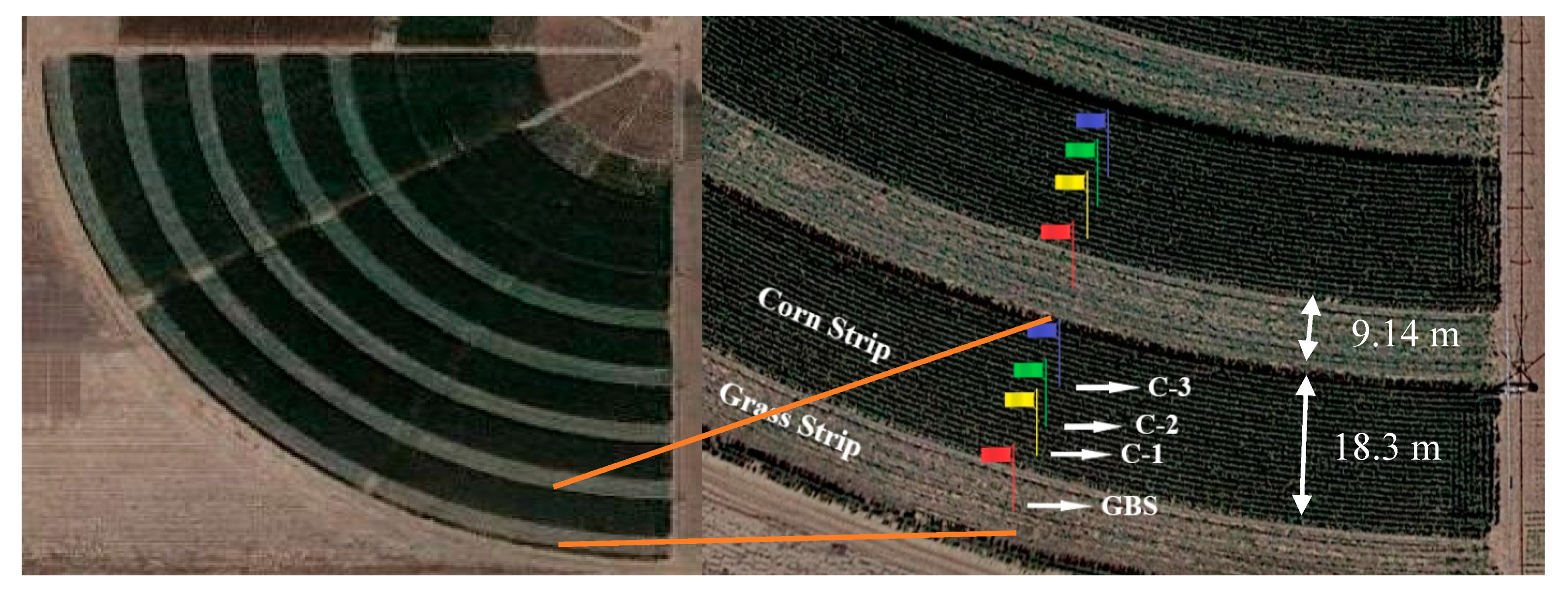
2.1. Study Site and Experimental Design

The study was conducted at the New Mexico State University Agricultural Science Center at Clovis, NM (34°35′ N, 103°12′ W; elevation 1348 m) in 2019. The study plots were established in 2016 with five perennial grass buffer strips (9.14 m wide) alternating with five corn strips of 18.3 m width in a 3.88 ha quarter circle area under an irrigation pivot. The study area has a semiarid climate with an average annual rainfall of 470 mm and the average yearly maximum and minimum temperatures of 22 °C and 6.56 °C, respectively. The soil of the experimental site is classified as Olton clay loam (fine, mixed, superactive, thermic Aridic Paleustolls) in the Soil Taxonomy [30] and Kastanozems in the World Reference Base for soil classification.
This study was conducted in four grass strips, at 1.52, 4.57, and 9.14 m distances from the edges of each grass strip in the adjacent corn strip (Figure 1). The soil sampling locations, at the center of grass buffer strips (GBS), and at 1.52 m (C-1), 4.57 m (C-2), and 9.14 m (C-3) from grass edges in corn strips were the four treatments, while four grass buffer strips and four corn strips constituted the four replications in this study.

2.2. Corn Planting and Grass Management

A mixture of six perennial grasses was sown on 9 August 2016, which included four warm-season grasses and two cool-season grasses. Warm-season grasses were Switchgrass (Panicum virgatum), Big Bluestem (Andropogon gerardi), Sideoats Grama (Bouteloua curtipendula), Indiangrass (Sorghastrum nutans), and Sand Bluestem (Andropogon hallii) and two cool-season grasses were Tall Wheatgrass (Thinopyrum ponticum) and Western Wheatgrass (Pascopyrum smithii). Irrigation applied to the grasses was 773 mm in 2016/17 for grass establishment and 122 and 117 mm in 2018 and 2019, respectively. More water was needed at the beginning to establish the grasses. The grasses were mowed to 10 cm from ground and bailed once in August 2018 and 2019.
Corn (Zea mays L.) variety Pioneer 1151 AquaMax was sown in the second week of May each year at a seeding rate of 54,363 seeds ha−1. Corn plots were fertilized with 207 kg ha−1 nitrogen (N), 90 kg ha−1 phosphorus (P), 33 kg ha−1 sulfur (S), and 9.35 kg ha−1 zinc (Zn) a few days before planting each year. Total irrigation water applied to the corn throughout the growing season was 491, 306, and 305 mm in 2017, 2018, and 2019, respectively. The corn strips were maintained with conventional tillage in which fields were first tilled with a disk in the winter followed by plowing to the depth of 23 cm by a DMI Ripper in early spring, and land finisher in May, a week before corn planting. Corn was planted with a John Deere four-row planter. Herbicides Balance Flexx (0.15 L ha−1), Atrazine (2.34 L ha−1), and Brawl 2 (1.75 L ha−1) were applied a day before planting. Oberon 4 SC (0.58 L ha−1), Stratego DIY (0.36 L ha−1), and Stomach (0.83 L ha−1) were applied on July 24 for weed control. To control the two-spotted spider mite (Tetranychus urticae), Comite II was applied at a rate of 3.9 L ha−1 in September. Corn was harvested in mid-October at physiological maturity.

2.3. Soil Sampling and Laboratory Analysis

Soil samples were collected in spring, summer, and fall of 2019. Spring soil samples were collected on May 31 (22 days after planting), summer sampling was done on July 16, and the fall sampling on October 24. Four soil cores were collected from four random locations in the middle of the grass strips and four cores at each distance from the edge of the grass strip using a core sampler of 3.18 cm inner diameter. Since corn was planted in 0.76 m row spacing, we collected two cores from the nearest crop row and two cores from central spots between the crop rows. The four cores were homogenized, composited by depth (0–10 cm and 10–20 cm) for each plot, brought to the laboratory, and stored at 4 °C in a refrigerator till laboratory analysis, which was done within two weeks of soil sampling. For soil bulk density, four cores from each sampling location were collected with a soil core sampler of 2.25 cm inner diameter up to 20 cm depth and divided into 0–10 and 10–20 cm depths. Soils were oven-dried and weighed to measure the dry bulk density in 0–10 and 10–20 cm depths. The average bulk density value was 1.25 ± 0.01 g cm−3 for 0–10 cm and 1.36 ± 0.01 g cm−3 for 0–20 cm depths and was consistent among treatments. These values were used for calculating soil measurements in kg ha−1 for each depth, but the seasonal variation in bulk density was not measured.
Laboratory analysis included inorganic N, PCM, potential nitrogen mineralization (PNM), labile organic nitrogen (LON), MBC, wet aggregate stability (WAS), SOC, TSN, gravimetric soil water content, soil pH, EC, and CEC. Inorganic N was analyzed as a sum of KCl extractable NO3− and NH4+ in an automated flow injection N analyzer (Timberline Instrument, LLC). In this method, approximately 5 g of soil was extracted in 25 mL 1 M potassium chloride (KCl). Soil PCM was measured by aerobic incubation of approximately 22 g soil at field capacity moisture (23% v/v) in a 1 L mason jar for 72 h and taking measurements of CO2 emissions [31] in an infrared gas analyzer (LI-830, Licor Inc). After 72 h, approximately 5 g of subsamples were extracted with KCl as described for inorganic N. The LON was measured by boiling the 5 g soil sample for four hours with 25 mL 1 M KCl in a Pyrex glass tube in a 100 °C water bath. After boiling, the extract was filtered and then NO3 and NH4+ were analyzed as inorganic N [32]. For soil MBC measurement, 10 g of soil samples were fumigated for 48 h with chloroform (CHCl3) and then incubated for 72 h using the protocol for PCM estimation [33]. Soil pH and EC were determined on a 1:1 soil to water suspension using electrodes. Soil CEC was determined by shaking soil with ammonium acetate (NH4OAc) for 16 h and determining the ammonium (NH4+) concentration exchanged with cations [34].
After all biochemical analyses, remaining soil samples were air-dried and sieved through a 4 mm sieve and prepared for WAS. Soil samples of 2–4 mm size were used for WAS measurement using a Cornell Sprinkler Infiltrometer [35]. The SOC and TSN were analyzed using the dry combustion method (Leco Corporation, St. Joseph, MI, USA).

2.4. Greenhouse Gas Measurements

The CO2 and N2O emissions were measured using an EGM-5 portable CO2 gas analyzer (PP Systems, Amesbury, MA) and MIRA Pico CO/N2O portable analyzer (Aeris Technology, Hayward, CA). For this method, a polyvinyl chloride (PVC) ring of 10 cm height and 10 cm inside diameter was installed in each plot up to 9 cm deep into the soil. It was installed in May after planting corn and occasionally removed for field operations (fertilization, spaying, etc.) and reinstalled immediately afterward. The frequency of gas sampling was once per week throughout the growing season. Sampling occurred between 0900 and 1100 h to reduce variability in CO2 and N2O flux due to diurnal fluctuation in temperature [36], and sampling was not conducted until after 24 h in case any rainfall or other soil disturbance events occurred. Plants or weeds inside the PVC ring were hand clipped or removed before each sampling to avoid CO2 gas contribution from aboveground plant parts. A soil respiration gas chamber of 15 cm height and 10 cm diameter was installed on the top of the PVC ring each time while taking the gas readings and waited for 5 min to take the CO2 and N2O gas readings. Gas samples were collected from the chamber headspace using an SRC-2 Soil Respiration Chamber connected to the EGM-5 analyzer and MIRA Pico Analyzer. Net flux was calculated by subtracting the air CO2 and N2O concentration from measured values. Both CO2 and N2O give the measurement in ppm by volume. Gas emission (R) was calculated using the following equation:
R   =   G n G 0 T n   ×   V A
where R is the gas emission rate (CO2/N2O flux in g m−2 h−1), G0 is the gas concentration (CO2/N2O) at the time of gas chamber installation (T = 0), Gn is the gas concentration at time Tn (5 min), A is the area of soil exposed in m2, and V is the system volume in m3. The cumulative emission of CO2-C and N2O-N was estimated by linear interpolation of weekly emission rates and numerical integration of individual data points. Soil and air temperatures (°C) and soil moisture (%) were also monitored from the 0–0.05 m depth at the time of gas flux measurements using a hydra probe (Stevens Water Monitoring Systems, Portland, OR) attached to the EGM-5 analyzer. Cumulative emissions of CO2 and N2O throughout the growing season were calculated by linear integration of the weekly measurements and summing the weekly emissions data for the entire study period.

2.5. Statistical Analysis

The treatments and sampling depth effects on soil properties were analyzed using the PROC MIXED procedure in SAS (v 9.4, SAS Institute, Cary, NC) for a randomized complete block experiment. The analysis used treatments and depths as fixed effects and replications as a random term. Similarly, the CO2 and N2O emissions were analyzed using the PROC MIXED procedure in SAS for a randomized complete block experiment with treatment and sampling date as the fixed effect and replication as a random term in the model. The CO2 and N2O emissions data did not meet the criteria for the normality of variance. Therefore, the data were log-transformed for statistical analysis but presented later in the original scale. Cumulative emissions of CO2, N2O, and total CO2-eq for the whole growing season were analyzed using the PROC MIXED model in SAS with treatment as fixed effects and replication as a random effect. All statistical analyses were performed at α ≤ 0.05 and means were separated using Tukey’ test.

3. Results

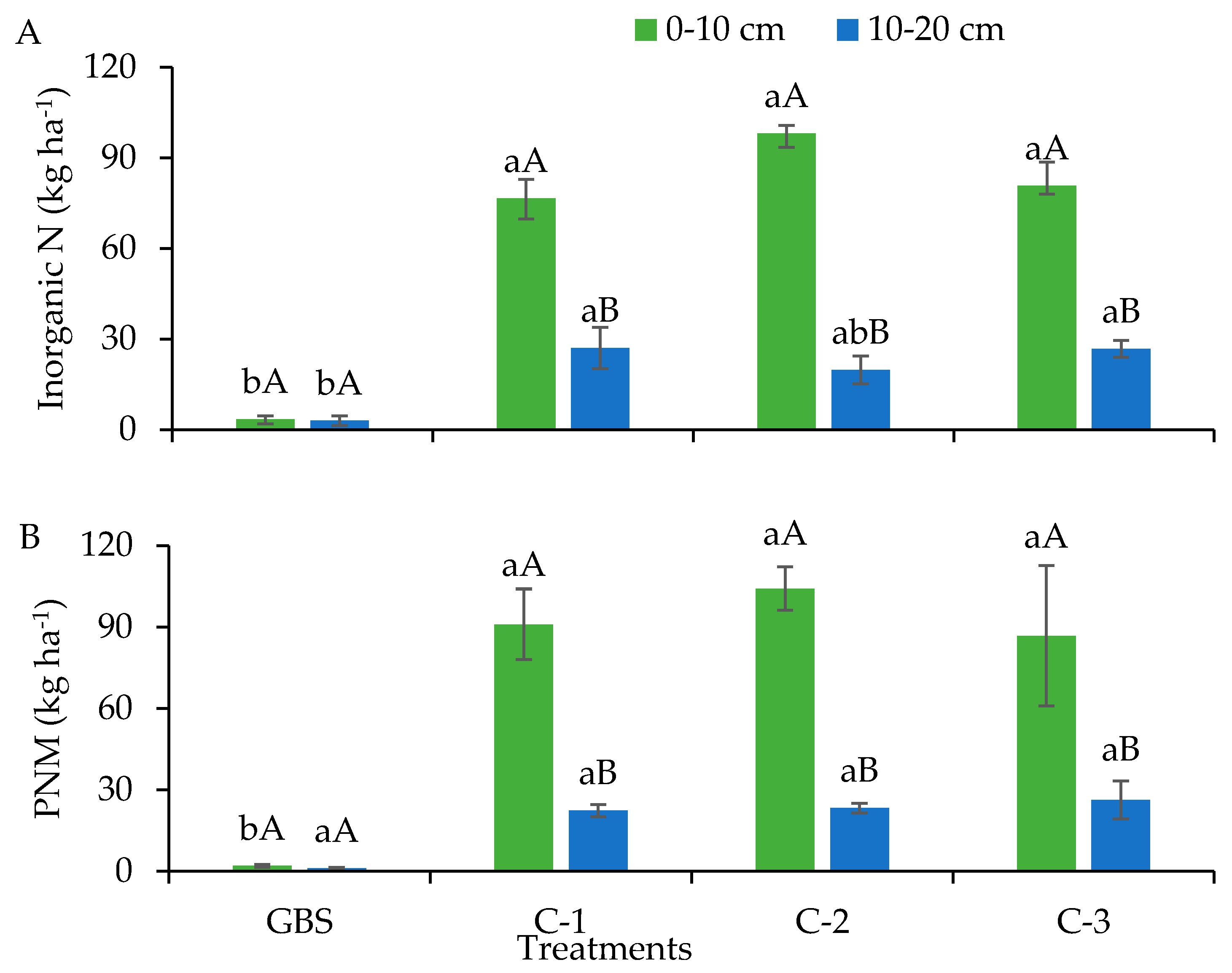
3.1. Soil Nitrogen Pools

Corn strips had significantly higher inorganic N than GBS in spring, irrespective of the sampling locations within corn strips at the 0–10 cm depth, as shown in Figure 2A. At the 10–20 cm depth, C-1 and C-3 had significantly higher inorganic N than GBS in the summer sampling. Among depths, the 0–10 cm soil had 238% and 108% greater inorganic N than the 10–20 cm depth in spring and summer samplings, respectively. In summer, inorganic N averaged over two depths in C-2 was significantly greater than GBS, while it was not significantly different from C-1 and C-3. Soil inorganic N was not significantly different among the treatments in fall, as shown in Table 1.
In spring, PNM was significantly higher in corn plots than GBS, mainly due to the difference in PNM content in the 0–10 cm soil, as shown in Figure 2B. When averaged for two depths, the C-2 had significantly higher PNM (11.0 kg ha−1) than GBS in summer and fall, but no significant difference was observed among C-1, C-3, and GBS. The 0–10 cm soil had 288% higher PNM than the 10–20 cm soil in spring, while it had only 69% higher PNM than the 10–20 cm soil in summer and no difference between soil depths in fall.
Soil samples collected in spring had significantly higher LON in corn strips than GBS, irrespective of sampling locations within corn strips. In summer, LON in C-2 and C-3 were considerably higher than GBS, but there was no difference in LON between C-1 and GBS. Fall samples did not show a significant difference in LON among treatments. Among depths, LON in 0–10 cm was 204% more than the 10–20 cm depth, which was 20.88 kg ha−1 in spring. The 0–10 cm soil depth had a 15% and 11% higher LON than the 10–20 cm soil with values 12.83 and 7.38 kg ha−1 in summer and fall, respectively, as shown in Table 1.
Soil TSN did not differ significantly among treatments, irrespective of the sampling season, but the 0–10 cm soil had 20%, 11%, and 11% higher TSN than the 10–20 cm soil in spring, summer, and fall samples, respectively.

3.2. Soil Carbon Pools

Soil PCM differed significantly among treatments in spring and summer. In spring, GBS had 99.9% higher PCM than corn strips (83.80 kg ha−1), irrespective of sampling locations. The 0–10 cm soil had 80.7% more PCM than the 10–20 cm soil (37.33 kg ha−1). In summer, PCM was 56.2% and 52.5% higher in GBS than in C-1 and C-3, and not different than C-2. In the fall, there was no significant difference among treatments in PCM. Among soil depths, the 0–10 cm soil depth had 32.1% and 113% more PCM than 10–20 cm in summer (39.05 kg ha−1) and fall (12.76 kg ha−1), respectively, as shown in Table 2.
Soil MBC was 52.5% and 36.7% higher in GBS than in C-1 and C-2 but did not significantly differ from C-3 in spring, as shown in Table 2. The MBC was 50.3% more in 0–10 cm than in the 10–20 cm soil (293.4 kg ha−1). In summer and fall, MBC did not differ among the treatments, and it was 16.2% more in 0–10 cm than in the 10–20 cm depth (476.5 kg ha−1) in summer.
The SOC content did not differ significantly among the treatments in any sampling when averaged over two depths, while the 0–10 cm soil had 22.1%, 7.96%, and 17.6% more SOC than the 10–20 cm soil in spring, summer, and fall with values of 11.43, 12.06, and 10.81 Mg ha−1, respectively.

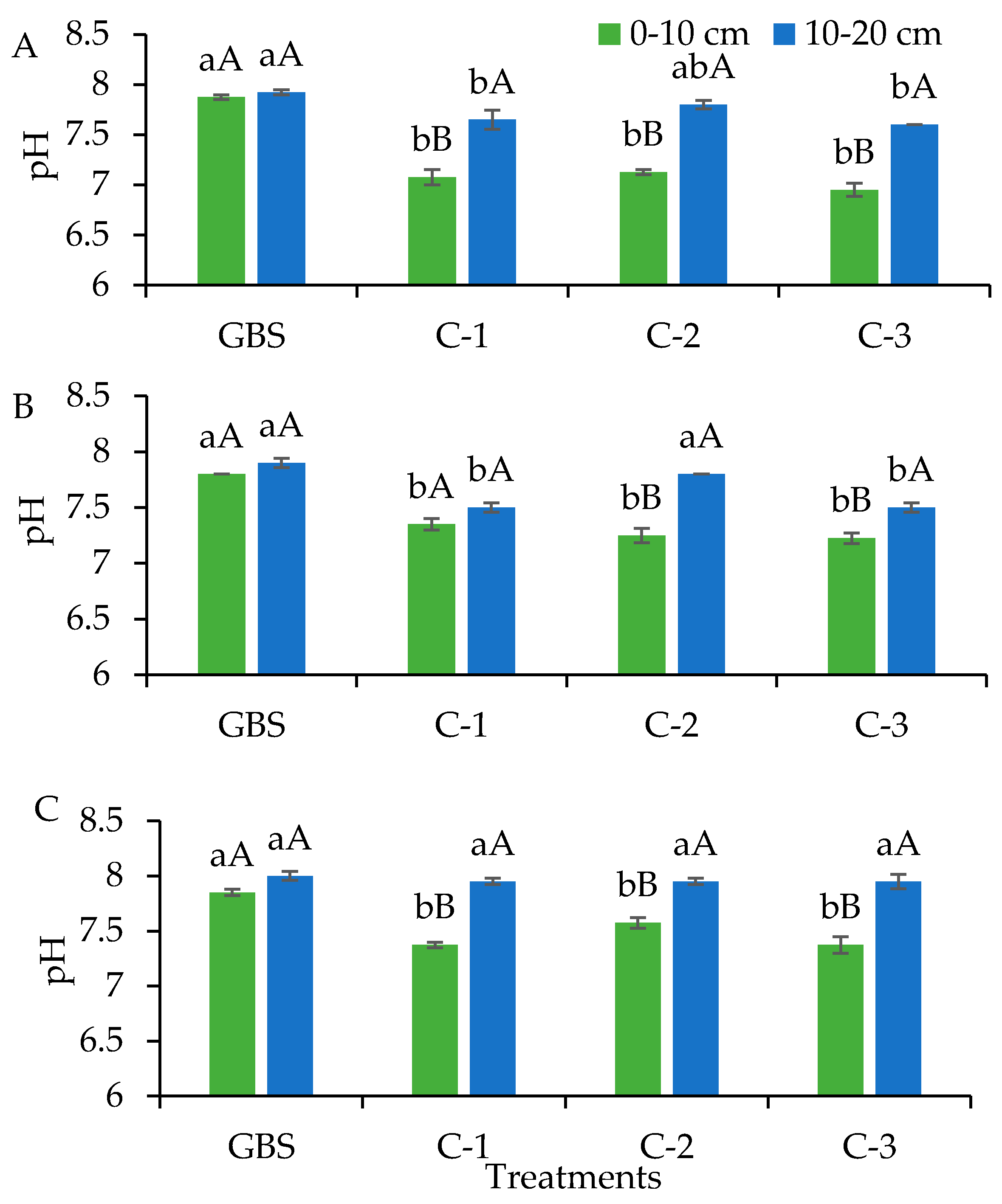
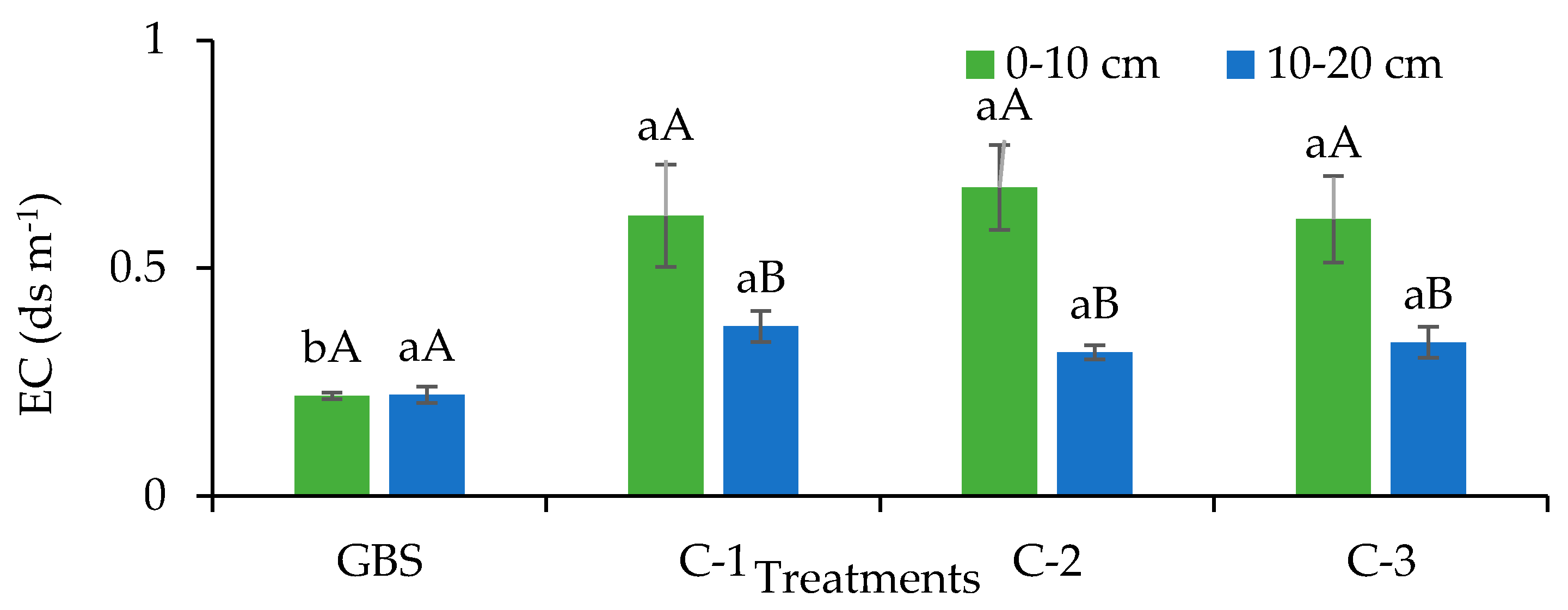
3.3. Other Soil Properties

Soil pH was significantly different between treatments at all three samplings (spring, summer, and fall). Considering the 0–10 cm soil depth, GBS had higher pH than corn strips, irrespective of sampling location, in spring, summer, and fall, respectively. At the 10–20 cm depth, GBS had higher pH than C-1 and C-3 in spring but no significant difference with C-2. In summer, GBS had a higher pH than C-1 and C-3 but no significant difference with C-2. There was no significant difference among treatments in soil pH at the 10–20 cm depth in fall. Among depths, soil pH was lower in 0–10 cm than in 10–20 cm with values 7.26, 7.41, and 7.54 in 0–10 cm and 7.74, 7.68, and 7.96 in 10–20 cm in spring, summer, and fall, respectively, as shown in Table 3 and Figure 3.
In spring, GBS had significantly lower EC (0.22 ds m−1) than corn strips at the 0–10 cm depth but no significant difference among the sampling locations within the corn strips. There was no significant difference among the treatments at the 10–20 cm depth, as shown in Figure 4. In summer and fall sampling, there was no significant difference among the treatments at any of the soil depths. Soil CEC did not differ significantly among the treatments in any of the sampling seasons, as shown in Table 3.
The WAS did not differ significantly among the treatments in spring and summer. In the fall, WAS gave significantly higher stability in GBS (39.3%) than in C-1 (33.8%). Sampling locations in corn strips were not different in WAS in fall. Among treatments, the 0–10 cm soil had 16.9% more WAS than the 10–20 cm soil in summer, as shown in Table 4.

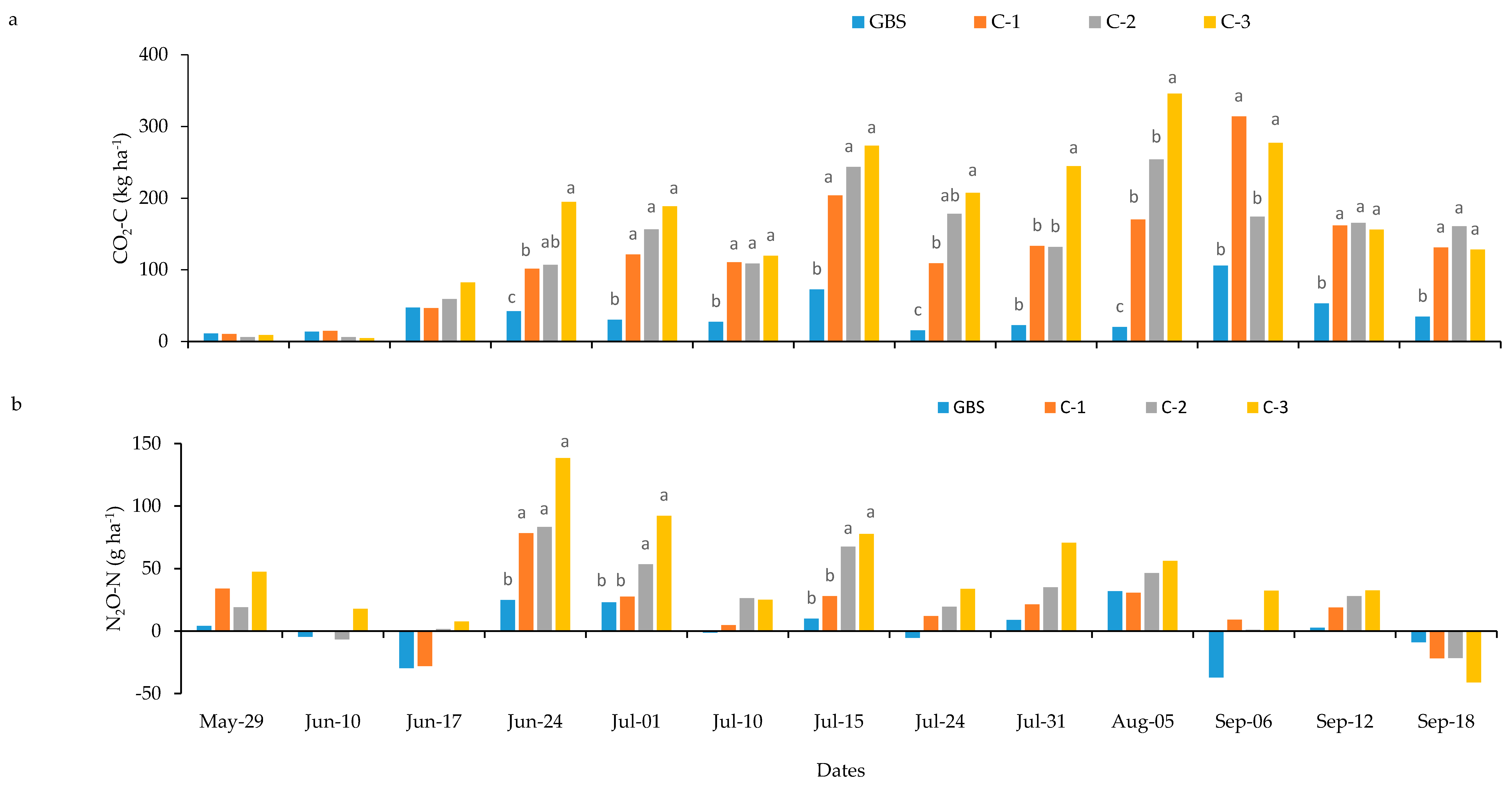
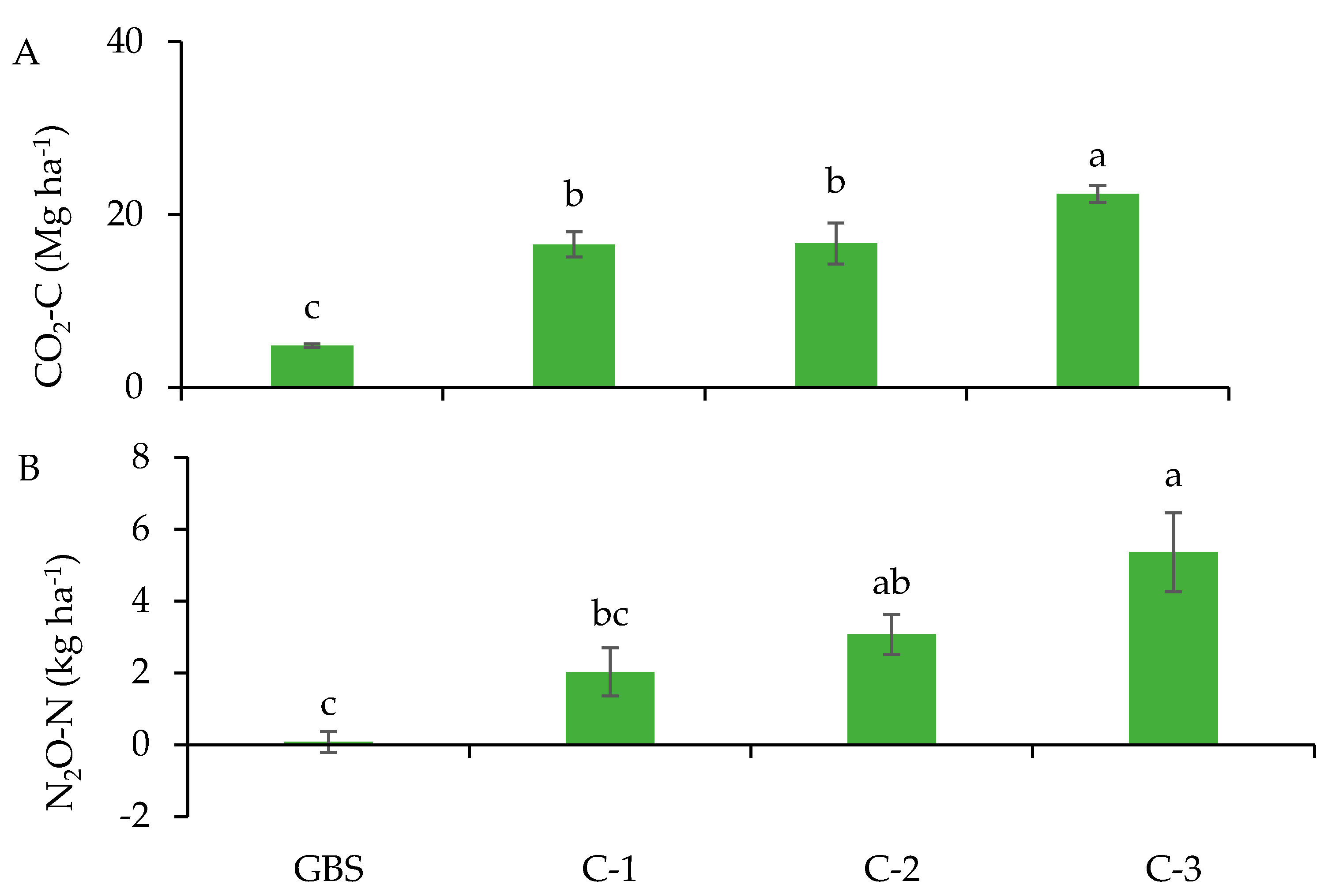
3.4. Greenhouse Gas Emissions

Greenhouse gas emissions varied among the treatments, and it was higher during summer and fall for all the treatment plots, as shown in Figure 5a, than in the GBS. Grass buffer strip treatment had the lowest cumulative CO2-C emission (4.83 Mg ha−1), and the emission increases with distance from the grass edge in the corn strip from C-1 to C-3, as shown in Figure 6a. Among the sampling locations within the corn strip, C-3 had the highest total emissions of CO2-C and was 35.3% higher than C-1 and 34.4% higher than C-2.
GBS had the lowest N2O-N emission (0.08 kg ha−1), and the emission increases with increasing distance from the edge almost linearly, as shown in Figure 5b. Cumulative N2O-N emission was significantly higher in C-2 (3.08 kg ha−1), and C-3 (5.36 kg ha−1) than GBS (0.08 kg ha−1), but C-1 (2.03 kg ha−1) was not significantly different than the GBS. C-3 had the highest N2O-N emission (5.36 kg ha−1), which was considerably higher than GBS (0.08 kg ha−1) and C-1 (2.03 kg ha−1), as shown in Figure 6b.

4. Discussion

Introducing grass buffer strips in irrigated corn production under center-pivot influenced soil C and N cycling. Our observation of significantly lower amounts of inorganic N, PNM, and LON in GBS than in corn strips suggested grass strips are N limited. In addition, the N lost from the edge of grass strip may have been utilized by grass, which helped with better grass growth at the edge and thereby maximized ecosystem services such as soil C sequestration and nutrient cycling. Specifically, significant difference in inorganic N in corn strips and GBS was observed in spring sampling, immediately after fertilizer application in corn. N fertilizer often increases inorganic N immediately after field application. In our study, corn strips received 207 kg ha−1 N three weeks before the spring sampling. Inorganic N was higher only in C-2 and C-3 in summer. Inorganic N, PNM, and LON contents were considerably less in fall than earlier sampling dates, mostly because of the crop uptake of N. No difference among treatments was observed in fall sampling. Despite seasonal variations and treatment differences in labile N components, total N stock did not differ between the GBS and corn strips because most of the fertilizer N released in soils is either used by crops or lost to the atmosphere as N2O fluxes.
Significantly higher PCM in GBS than corn strips, mostly in spring and summer sampling, and no difference between sampling locations within corn strips indicate a higher amount of labile substrates and thereby microbial activity under grasses than under corn, but there were minimum edge effects of grasses on PCM concentration in corn strips. Soil N utilized from the edge of corn and grasses may add more soil C in the edges. We collected soil samples only from the center of grass strips, and the edge effects are unknown. Previous studies comparing grasslands and croplands reveal N limitation in grassland, but they had higher PCM and total soil C than croplands [16,20,37]. Grasses often have deeper and denser root systems than annual crops, which contributes to greater root-derived C under grasses than under annual crops [38]. The MBC was also higher in GBS than corn strips in spring sampling, supporting more biological activity under grass strips than corn strips in the spring. The trend of PCM and MBC was the highest amounts in spring, followed by lower amounts in summer and fall. The MBC and PCM values were only numerically higher during summer and fall samplings, suggesting that biological indicators of soil health are sensitive and seasonally variable. Increases in their concentrations due to grass buffer strips may not reflect increased SOC storage in the first few years of grass establishment as we observed no significant difference in SOC among the treatments. It may take several years to increase SOC in semiarid agroecosystems. Earlier studies suggest at least 12 years is needed to observe a significant increase in SOC storage due to grassland transition from croplands [15,16,17,25].
The cumulative CO2 and N2O emissions had a linear trend of increase as the distance from grass strip to sampling location in corn strips increased, which demonstrated the greatest edge effects of grass strips in GBS-integrated corn production systems. The CO2 emission was lowest in GBS and increased with increasing distance from the grass edge toward the middle of corn strips. Corn plots were maintained with conventional tillage, full irrigation, and soil test-based fertility management, while grass strips were not tilled since establishment and received no fertilizer and only a little irrigation for their establishment. The reduced emission of CO2 and N2O in grassland and in close distance from grassland is associated with alteration in soil moisture, temperature, and soil physicochemical properties in grass strips and close distance of grass strips in the crop strips. There might have been a lateral flow of nutrients and water on the edge of grass and corn and dense root systems of grasses utilized the water from corn strips in the close distance, reducing microbial and root respiration of C. Previous studies reported reduced microbial respiration of CO2 in low moisture conditions [39,40]. Reduced soil moisture also adversely affects the nitrification and denitrification loss of N2O from the soil [41,42]. Reduced GHGs and increased microbial biomass, as well as labile SOC components, suggest reallocation of resources, which in the long term can increase SOC and improve ecosystem services. In line with our observations, a study in Iowa demonstrated less CO2 and N2O emissions from grass-buffered corn production than systems without buffer strips [12]. The N2O-N emissions, in our study, had a clearer trend than CO2-C, with the highest emissions at the C-3 location (9.14 m distance).
Soil pH was lower in corn strips than GBS, possibly because of the fertilization in corn. A high N rate for several years acidifies soil [43], but there was no edge effect as indicated by no significant difference between sampling locations within corn strips. Lower pH in the 0–10 cm depth than the 10–20 cm depth in corn strips and no difference in pH between depths in GBS suggest fertilizer effects on pH in corn strips. Liquid N fertilizer was applied on the soil surface, which led to lower pH in the surface soil. Soils are typically alkaline in the southern High Plains; a small decrease in pH toward neutral pH supports better microbial activity, nutrient availability, and improved plant growth. However, the continuous application of a high rate of N fertilizer can cause soil acidification and negatively affect crop production [18,43]. Neutralization of alkaline salts with a change in pH can also increase soil EC, which in the short term (<5 years) increases the availability of mineral nutrients like potassium (K), calcium (Ca), and magnesium (Mg). However, it causes soil crusting, surface sealing, and negatively affects crop production in the long term [44]. We observed an increased EC in corn strips in spring sampling only, and EC values of all the treatments were in the non-saline range. Variation in pH and EC was minimal in grass strips, which in the long term could help in moderating soil conditions in corn strips and support improving soil health of the entire agroecosystem.

5. Conclusions

Circular grass buffer strips in center-pivot irrigation systems provide an opportunity to improve soil health and environmental quality by increasing labile C and N components, as early as three years of grass establishment. Apart from the grass buffer strips having lower CO2 and N2O emissions, it also reduced emissions at locations within the corn strips. The extent of emission reduction in the corn strip was linearly related to the distance from grass buffer strip. Total C and N stock did not vary between grass and corn strips, irrespective of the distance from the edge of the grass strip. Higher microbial biomass C was present in grass buffer compared to corn strips, indicating that microbial growth and SOC accumulation directly depend on the organic inputs. Grass buffer reduced CO2 and N2O emissions from irrigated corn production and improved environmental quality. The integrating circular grass buffer strips in center-pivot irrigated systems has the potential to improve soil health and ecosystem services in the southern High Plains of USA and similar agroecosystems across the world facing soil degradation and water limitation for irrigated crop production.

Author Contributions

Conceptualization, R.G. and S.V.A.; methodology, R.G.; field data collection and laboratory analysis, S.M.S.; resources, R.G. and S.V.A.; writing—original draft preparation, S.M.S. and R.G.; writing—review and editing, S.M.S., R.G., S.V.A., and O.J.I.; project administration, R.G. and S.V.A.; funding acquisition, R.G., S.V.A., and O.J.I.; All authors have read and agreed to the published version of the manuscript.

Funding

This research was funded by the USDA-NRCS and partly by the NMSU Agricultural Experiment Station. The study plots were established with funding from USDA-NIFA (grant # 2016-67019-25028).

Acknowledgments

Thanks to the staff of New Mexico State University Agricultural Science Center at Clovis, NM, for helping in the field and laboratory works of the study.

Conflicts of Interest

The authors declare no conflict of interest. The funders had no role in the design of the study; in the collection, analyses, or interpretation of data; in the writing of the manuscript, or in the decision to publish the results.

References

  1. Scanlon, B.R.; Faunt, C.C.; Longuevergne, L.; Reedy, R.C.; Alley, W.M.; McGuire, V.L.; McMahon, P.B. Groundwater depletion and sustainability of irrigation in the US High Plains and Central Valley. Proc. Natl. Acad. Sci. USA 2012, 109, 9320–9325. [Google Scholar] [CrossRef] [PubMed] [Green Version]
  2. Lee, J.A.; Baddock, M.C.; Mbuh, M.J.; Gill, T.E. Geomorphic and land cover characteristics of aeolian dust sources in West Texas and eastern New Mexico, USA. Aeolian Res. 2012, 3, 459–466. [Google Scholar] [CrossRef]
  3. Lee, J.; Gill, T.E. Multiple causes of wind erosion in the Dust Bowl. Aeolian Res. 2015, 19, 15–36. [Google Scholar] [CrossRef]
  4. Sophocleous, M. Retracted: Conserving and Extending the Useful Life of the Largest Aquifer in North America: The Future of the High Plains/Ogallala Aquifer. Ground Water 2012, 50, 831–839. [Google Scholar] [CrossRef] [PubMed]
  5. Hornbeck, R.; Keskin, P. The Historically Evolving Impact of the Ogallala Aquifer: Agricultural Adaptation to Groundwater and Drought. Am. Econ. J. Appl. Econ. 2014, 6, 190–219. [Google Scholar] [CrossRef] [Green Version]
  6. Udawatta, R.P.; Garrett, H.E.; Kallenbach, R.L. Agroforestry and grass buffer effects on water quality in grazed pastures. Agrofor. Syst. 2010, 79, 81–87. [Google Scholar] [CrossRef]
  7. Wauters, E.; Bielders, C.L.; Poesen, J.; Govers, G.; Mathijs, E.E. Adoption of soil conservation practices in Belgium: An examination of the theory of planned behaviour in the agri-environmental domain. Land Use Policy 2010, 27, 86–94. [Google Scholar] [CrossRef]
  8. Xiao, B.; Wang, Q.; Wang, H.; Wu, J.-Y.; Yu, D. The effects of grass hedges and micro-basins on reducing soil and water loss in temperate regions: A case study of Northern China. Soil Tillage Res. 2012, 122, 22–35. [Google Scholar] [CrossRef]
  9. Josefsson, J.; Berg, A.; Hiron, M.; Pärt, T.; Eggers, S. Grass buffer strips benefit invertebrate and breeding skylark numbers in a heterogeneous agricultural landscape. Agric. Ecosyst. Environ. 2013, 181, 101–107. [Google Scholar] [CrossRef]
  10. Kumar, S.; Anderson, S.H.; Udawatta, R.P. Agroforestry and Grass Buffer Influences on Macropores Measured by Computed Tomography under Grazed Pasture Systems. Soil Sci. Soc. Am. J. 2010, 74, 203–212. [Google Scholar] [CrossRef]
  11. Paudel, B.R.; Udawatta, R.P.; Anderson, S.H. Agroforestry and grass buffer effects on soil quality parameters for grazed pasture and row-crop systems. Appl. Soil Ecol. 2011, 48, 125–132. [Google Scholar] [CrossRef]
  12. Moore, K.J.; Anex, R.P.; Elobeid, A.E.; Fei, S.-Z.; Flora, C.B.; Goggi, A.S.; Jacobs, K.L.; Jha, P.; Kaleita, A.L.; Karlen, D.L.; et al. Regenerating Agricultural Landscapes with Perennial Groundcover for Intensive Crop Production. Agronomy 2019, 9, 458. [Google Scholar] [CrossRef] [Green Version]
  13. Angadi, S.V.; Gowda, P.; Cutforth, H.W.; Idowu, O.J. Circles of live buffer strips in a center pivot to improve multiple ecosystem services and sustainability of irrigated agriculture in the southern Great Plains. J. Soil Water Conserv. 2016, 71, 44–49. [Google Scholar] [CrossRef] [Green Version]
  14. Iqbal, J.; Parkin, T.B.; Helmers, M.; Zhou, X.; Castellano, M.J. Denitrification and Nitrous Oxide Emissions in Annual Croplands, Perennial Grass Buffers, and Restored Perennial Grasslands. Soil Sci. Soc. Am. J. 2014, 79, 239–250. [Google Scholar] [CrossRef] [Green Version]
  15. Breuer, L.; Huisman, J.; Keller, T.; Frede, H.-G. Impact of a conversion from cropland to grassland on C and N storage and related soil properties: Analysis of a 60-year chronosequence. Geoderma 2006, 133, 6–18. [Google Scholar] [CrossRef]
  16. Ghimire, R.; Thapa, V.R.; Cano, A.; Acosta-Martinez, V. Soil organic matter and microbial community responses to semiarid croplands and grasslands management. Appl. Soil Ecol. 2019, 141, 30–37. [Google Scholar] [CrossRef]
  17. Don, A.; Scholten, T.; Schulze, E.-D. Conversion of cropland into grassland: Implications for soil organic-carbon stocks in two soils with different texture. J. Plant Nutr. Soil Sci. 2009, 172, 53–62. [Google Scholar] [CrossRef]
  18. Jiao, Y.; Xu, Z.; Zhao, J.; Yang, W. Changes in soil carbon stocks and related soil proper-ties along a 50-year grassland-to-cropland conversion chronosequence in an agro-pastoral ecotone of Inner Mongolia, China. J. Arid. Land 2012, 4, 420–430. [Google Scholar] [CrossRef] [Green Version]
  19. Yu, P.; Liu, S.; Han, K.; Guan, S.; Zhou, D. Conversion of cropland to forage land and grassland increases soil labile carbon and enzyme activities in northeastern China. Agric. Ecosyst. Environ. 2017, 245, 83–91. [Google Scholar] [CrossRef]
  20. Bronson, K.F.; Zobeck, T.; Chua, T.T.; Acosta-Martinez, V.; Van Pelt, R.S.; Booker, J.D. Carbon and Nitrogen Pools of Southern High Plains Cropland and Grassland Soils. Soil Sci. Soc. Am. J. 2004, 68, 1695–1704. [Google Scholar] [CrossRef] [Green Version]
  21. Glover, J.D.; Reganold, J.P.; Bell, L.W.; Borevitz, J.O.; Brummer, E.C.; Buckler, E.S.; Cox, C.M.; Cox, T.S.; Crews, T.E.; Culman, S.W.; et al. Increased Food and Ecosystem Security via Perennial Grains. Science 2010, 328, 1638–1639. [Google Scholar] [CrossRef] [PubMed] [Green Version]
  22. Mitchell, D.; Zhou, X.; Parkin, T.B.; Helmers, M.; Castellano, M.J. Comparing Nitrate Sink Strength in Perennial Filter Strips at Toeslopes of Cropland Watersheds. J. Environ. Qual. 2015, 44, 191–199. [Google Scholar] [CrossRef] [PubMed] [Green Version]
  23. Culman, S.W.; Dupont, S.; Glover, J.; Buckley, D.H.; Fick, G.; Ferris, H.; Crews, T. Long-term impacts of high-input annual cropping and unfertilized perennial grass production on soil properties and belowground food webs in Kansas, USA. Agric. Ecosyst. Environ. 2010, 137, 13–24. [Google Scholar] [CrossRef]
  24. Kim, D.-G.; Isenhart, T.; Parkin, T.B.; Schultz, R.C.; Loynachan, T.E. Methane Flux in Cropland and Adjacent Riparian Buffers with Different Vegetation Covers. J. Environ. Qual. 2010, 39, 97–105. [Google Scholar] [CrossRef] [Green Version]
  25. Evrendilek, F.; Celik, I.; Kilic, S. Changes in soil organic carbon and other physical soil properties along adjacent Mediterranean forest, grassland, and cropland ecosystems in Turkey. J. Arid. Environ. 2004, 59, 743–752. [Google Scholar] [CrossRef]
  26. Masarik, K.C.; Norman, J.M.; Brye, K.R. Long-Term Drainage and Nitrate Leaching below Well-Drained Continuous Corn Agroecosystems and a Prairie. J. Environ. Prot. 2014, 5, 240–254. [Google Scholar] [CrossRef] [Green Version]
  27. Berthrong, S.T.; Piñeiro, G.; Jobbágy, E.G.; Jackson, R.B. Soil C and N changes with afforestation of grasslands across gradients of precipitation and plantation age. Ecol. Appl. 2012, 22, 76–86. [Google Scholar] [CrossRef] [Green Version]
  28. Udawatta, R.P.; Jose, S. Carbon Sequestration Potential of Agroforestry Practices in Temperate North America. In Carbon Sequestration Potential of Agroforestry Systems; Springer Science Business Media: Berlin, Germany, 2011; pp. 17–42. [Google Scholar]
  29. Gopalakrishnan, G.; Negri, M.C.; Salas, W. Modeling biogeochemical impacts of bioenergy buffers with perennial grasses for a row-crop field in I llinois. Gcb Bioenergy 2012, 4, 739–750. [Google Scholar] [CrossRef]
  30. Web Soil Survey. Available online: http://websoilsurvey.nrcs.usda.gov (accessed on 21 February 2013).
  31. Zibilske, L. Carbon mineralization 1. In Methods of Soil Analysis: Part 2—Microbiological and Biochemical Properties; Wiley: Hoboken, NJ, USA, 1994; pp. 835–863. [Google Scholar]
  32. Gianello, C.; Bremner, J.M. A simple chemical method of assessing potentially available organic nitrogen in soil. Commun. Soil Sci. Plant Anal. 1986, 17, 195–214. [Google Scholar] [CrossRef]
  33. Jenkinson, D.; Powlson, D. The effects of biocidal treatments on metabolism in soil—V. Soil Boil. Biochem. 1976, 8, 209–213. [Google Scholar] [CrossRef]
  34. Sparks, D.L.; Page, A.L.; Helmke, P.A.; Loeppert, R.H. (Eds.) Methods of Soil Analysis, Part 3: Chemical Methods; John Wiley & Sons: Hoboken, NJ, USA, 2020; Volume 14. [Google Scholar]
  35. Ogden, C.B.; Van Es, H.M.; Schindelbeck, R. Miniature Rain Simulator for Field Measurement of Soil Infiltration. Soil Sci. Soc. Am. J. 1997, 61, 1041–1043. [Google Scholar] [CrossRef]
  36. Parkin, T.B.; Kaspar, T.C. Temperature Controls on Diurnal Carbon Dioxide Flux. Soil Sci. Soc. Am. J. 2003, 67, 1763–1772. [Google Scholar] [CrossRef]
  37. Thapa, V.R.; Ghimire, R.; Mikha, M.M.; Idowu, O.J.; Marsalis, M.A. Land Use Effects on Soil Health in Semiarid Drylands. Agric. Environ. Lett. 2018, 3, 180022. [Google Scholar] [CrossRef]
  38. Sainju, U.M.; Allen, B.L.; Lenssen, A.W.; Ghimire, R. Root biomass, root/shoot ratio, and soil water content under perennial grasses with different nitrogen rates. Field Crop. Res. 2017, 210, 183–191. [Google Scholar] [CrossRef] [Green Version]
  39. Garten, C.; Classen, A.T.; Norby, R.J. Soil moisture surpasses elevated CO2 and temperature as a control on soil carbon dynamics in a multi-factor climate change experiment. Plant Soil 2008, 319, 85–94. [Google Scholar] [CrossRef]
  40. Davidson, E.A.; Belk, E.; Boone, R.D. Soil water content and temperature as independent or confounded factors controlling soil respiration in a temperate mixed hardwood forest. Glob. Chang Boil. 1998, 4, 217–227. [Google Scholar] [CrossRef] [Green Version]
  41. Schaufler, G.; Kitzler, B.; Schindlbacher, A.; Skiba, U.; Sutton, M.A.; Zechmeister-Boltenstern, S. Greenhouse gas emissions from European soils under different land use: Effects of soil moisture and temperature. Eur. J. Soil Sci. 2010, 61, 683–696. [Google Scholar] [CrossRef]
  42. Maag, M.; Vinther, F. Nitrous oxide emission by nitrification and denitrification in different soil types and at different soil moisture contents and temperatures. Appl. Soil Ecol. 1996, 4, 5–14. [Google Scholar] [CrossRef]
  43. Ghimire, R.; Machado, S.; Bista, P. Soil pH, Soil Organic Matter, and Crop Yields in Winter Wheat-Summer Fallow Systems. Agron. J. 2017, 109, 706–717. [Google Scholar] [CrossRef] [Green Version]
  44. Aizat, A.M.; Roslan, M.K.; Sulaiman, W.N.; Karam, D.S. The relationship between soil pH and selected soil properties in 48 years logged-over forest. Int. J. Environ. Sci. 2014, 4, 1129–1140. [Google Scholar]
Figure 1. Grass and corn strips in a center-pivot irrigation system and the sampling locations within each strip.
Sustainability 12 06014 g001
Figure 2. Soil inorganic N (A) and potential nitrogen mineralization (PNM) (B) in 0–10 and 10–20 cm depths in spring 2019. Different lowercase letters indicate a significant difference between treatments within the depth, and different uppercase letters indicate a significant difference between depths within the treatment. GBS, grass buffer strip, C-1, C-2, and C-3, sampling locations in corn strips at 1.52, 4.57, and 9.14 m away from the grass edge, respectively.
Sustainability 12 06014 g002
Figure 3. Soil pH under different treatments in spring (A), summer (B), and fall (C) in 0–10 and 10–20 cm depths. Different lowercase letters indicate significant differences among treatments within the depth, and different uppercase letters indicate a significant difference between depths within the treatment. GBS, grass buffer strip, and C–1, C-2, and C-3 represent sampling locations in corn strips at 1.52, 4.57, and 9.14 m away from the grass edge, respectively.
Sustainability 12 06014 g003
Figure 4. Soil EC as influenced by different treatments in spring soil sampling in two soil depths (0–10 cm and 10–20 cm). Different lowercase letters indicate a significant difference among the treatments within the depth, and different uppercase letters indicate a significant difference between the depths within the treatment. GBS, grass buffer strip, and C-1, C-2, and C-3 represent sampling locations in corn strips at 1.52, 4.57, and 9.14 m away from the grass edge, respectively.
Sustainability 12 06014 g004
Figure 5. CO2-C (a) and N2O-N (b) emissions during the growing season in 2019 under different treatments and sampling dates. Different lowercase letters indicate a significant difference among the treatments within a measurement date. The individual bar represents data in the original scale, but the means were separated on a log-transformed data. GBS, grass buffer strip, and C-1, C-2, and C-3 represent sampling locations in corn strips at 1.52, 4.57, and 9.14 m away from the grass edge, respectively.
Sustainability 12 06014 g005
Figure 6. Cumulative emission of CO2-C (A) and N2O-N (B) in different treatments. Different lowercase letters indicate a significant difference among the treatments within a measurement date. GBS, grass buffer strip, and C-1, C-2, and C-3 represent sampling locations in corn strips at 1.52, 4.57, and 9.14 m away from the grass edge, respectively.
Sustainability 12 06014 g006
Table 1. Inorganic N, potential nitrogen mineralization (PNM), labile organic nitrogen (LON), and total soil nitrogen (TSN) in different treatments in spring, summer, and fall 2019.
TreatmentsSpringSummerFall
Inorganic N (kg ha−1)
GBS3.21 ± 0.88 b0.64 ± 0.12 b1.83 ± 0.19
C-151.84 ± 10.31 a4.02 ± 0.91 ab1.74 ± 0.11
C-258.91 ± 15.00 a11.0 ± 3.27 a1.76 ± 0.12
C-353.80 ± 10.91 a7.99 ± 1.68 ab1.86 ± 0.12
PNM (kg ha−1)
GBS1.55 ± 0.37 b0.39 ± 0.10 b1.06 ± 0.04 b
C-156.69 ± 14.35 a6.64 ± 1.31 ab1.16 ± 0.04 ab
C-263.71 ± 15.74 a18.96 ± 5.02 a1.24 ± 0.03 a
C-356.53 ± 16.85 a13.94 ± 4.11 ab1.16 ± 0.04 ab
LON (kg ha−1)
GBS10.74 ± 2.56 b6.00 ± 0.50 b6.88 ± 0.47
C-155.61 ± 14.40 a10.73 ± 1.61 ab7.38 ± 0.65
C-252.94 ± 13.72 a19.26 ± 3.01 a8.50 ± 0.58
C-349.29 ± 15.31 a19.22 ± 1.66 a8.31 ± 0.41
TSN (Mg ha−1)
GBS1.30 ± 0.091.18 ± 0.031.12 ± 0.02
C-11.29 ± 0.041.20 ± 0.051.17 ± 0.04
C-21.31 ± 0.051.33 ± 0.031.23 ± 0.03
C-31.35 ± 0.061.32 ± 0.041.22 ± 0.06
Data presented as mean ± standard error followed by different lowercase letters indicate a significant difference between the treatments averaged over two depths (0–10 and 10–20 cm, n = 8). GBS, grass buffer strip, and C-1, C-2, and C-3 represent sampling locations in corn strips at 1.52, 4.57, and 9.14 m away from the grass edge, respectively.
Table 2. Potential carbon mineralization (PCM), soil organic carbon (SOC), and microbial biomass (MBC) in response to different treatments in spring, summer, and fall samplings.
TreatmentsSpringSummerFall
PCM (kg ha−1)
GBS83.80 ± 16.82 a58.26 ± 5.84 a24.01 ± 3.80
C-140.89 ± 5.59 b37.30 ± 2.66 b18.82 ± 4.18
C-241.30 ± 3.82 b47.51 ± 5.52 ab20.62 ± 3.14
C-343.59 ± 4.92 b38.20 ± 3.26 b16.44 ± 2.88
MBC (kg ha−1)
GBS465.37 ± 48.37 a560.62 ± 31.74442.60 ± 28.51
C-1305.24 ± 24.10 b490.59 ± 27.12385.93 ± 29.29
C-2340.47 ± 31.02 b518.84 ± 27.82389.10 ± 20.93
C-3357.93 ± 39.11 ab490.62 ± 35.27369.67 ± 35.31
SOC (Mg ha−1)
GBS13.83 ± 1.1611.87 ± 0.2211.14 ± 0.30
C-111.86 ± 0.4011.90 ± 0.3411.51 ± 0.50
C-212.19 ± 0.4513.21 ± 0.4411.86 ± 0.29
C-312.91 ± 0.7013.21 ± 0.3912.55 ± 0.95
Data presented as a mean ± standard error. Different lowercase letters indicate significant difference among the treatments averaged over two depths (0–10 and 10–20 cm, n = 8). GBS, grass buffer strip, and C-1, C-2, and C-3 represent sampling locations in corn strips at 1.52, 4.57, and 9.14 m away from the grass edge, respectively.
Table 3. Soil pH, electrical conductivity (EC), and cation exchange capacity (CEC) as influenced by grass buffer and distances from the grass edge in spring, summer, and fall.
TreatmentsSpringSummerFall
Soil pH
GBS7.90 ± 0.02 a7.85 ± 0.03 a7.93 ± 0.04 a
C-17.36 ± 0.12 c7.43 ± 0.04 c7.66 ± 0.11 b
C-27.46 ± 0.13 b7.53 ± 0.12 b7.76 ± 0.08 ab
C-37.28 ± 0.13 d7.36 ± 0.06 c7.66 ± 0.12 b
EC (ds m−1)
GBS0.22 ± 0.01 b0.19 ± 0.020.21 ± 0.01
C-10.49 ± 0.07 a0.23 ± 0.010.20 ± 0.01
C-20.50 ± 0.08 a0.33 ± 0.050.23 ± 0.01
C-30.47 ± 0.07 a0.30 ± 0.020.20 ± 0.02
CEC (meq 100 g−1)
GBS16.91 ± 0.3717.3 ± 0.4017.54 ± 0.28
C-117.95 ± 0.4017.18 ± 0.2717.15 ± 0.24
C-217.91 ± 0.4217.38 ± 0.3017.45 ± 0.46
C-317.29 ± 0.5017.40 ± 0.4617.60 ± 0.41
Data presented as mean ± standard error followed by different lowercase letters indicate a significant difference between the treatments averaged over two depths (0–10 and 10–20 cm, n = 8). GBS, grass buffer strip, and C-1, C-2, and C-3 represent sampling locations in corn strips at 1.52, 4.57, and 9.14 m away from the grass edge.
Table 4. Wet aggregate stability (WAS) as % in response to different treatments in spring, summer, and fall seasons averaged over two depths (0–10 and 10–20 cm).
TreatmentsSpringSummerFall
WAS (%)
GBS51.86 ± 6.2648.63 ± 3.2039.34 ± 1.79 a
C-154.13 ± 6.4947.45 ± 2.9533.80 ± 1.95 b
C-247.46 ± 6.7444.93 ± 1.9235.75 ± 1.75 ab
C-352.81 ± 5.3244.32 ± 2.3337.27 ± 1.73 ab
Data presented as a mean ± standard error. Different lowercase letters indicate significant difference among the treatments averaged over two depths (0–10 and 10–20 cm, n = 8). GBS, grass buffer strip, and C-1, C-2, and C-3 represent sampling locations in corn strips at 1.52, 4.57, and 9.14 m away from the grass edge, respectively.

