An Economic Order Quantity Stochastic Dynamic Optimization Model in a Logistic 4.0 Environment


Abstract
:1. Introduction
2. Literature Review
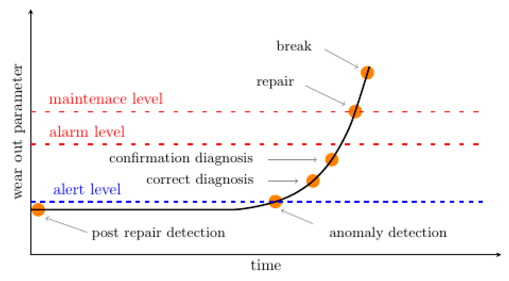
2.1. Faults and Analysis
2.2. Maintenance Strategy
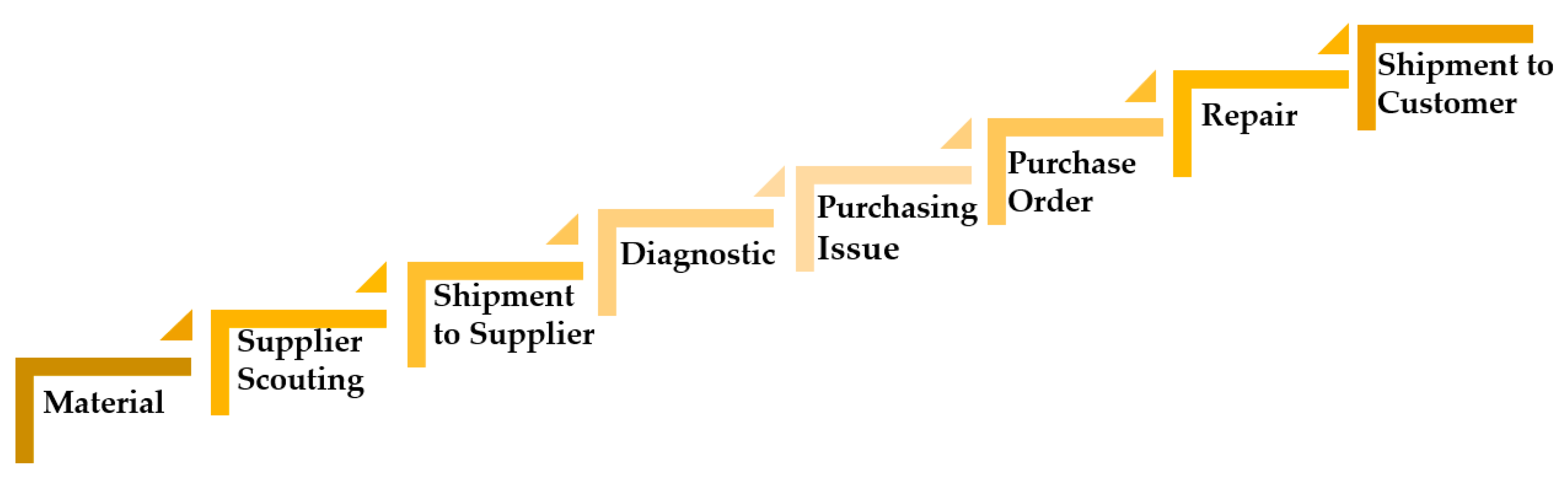
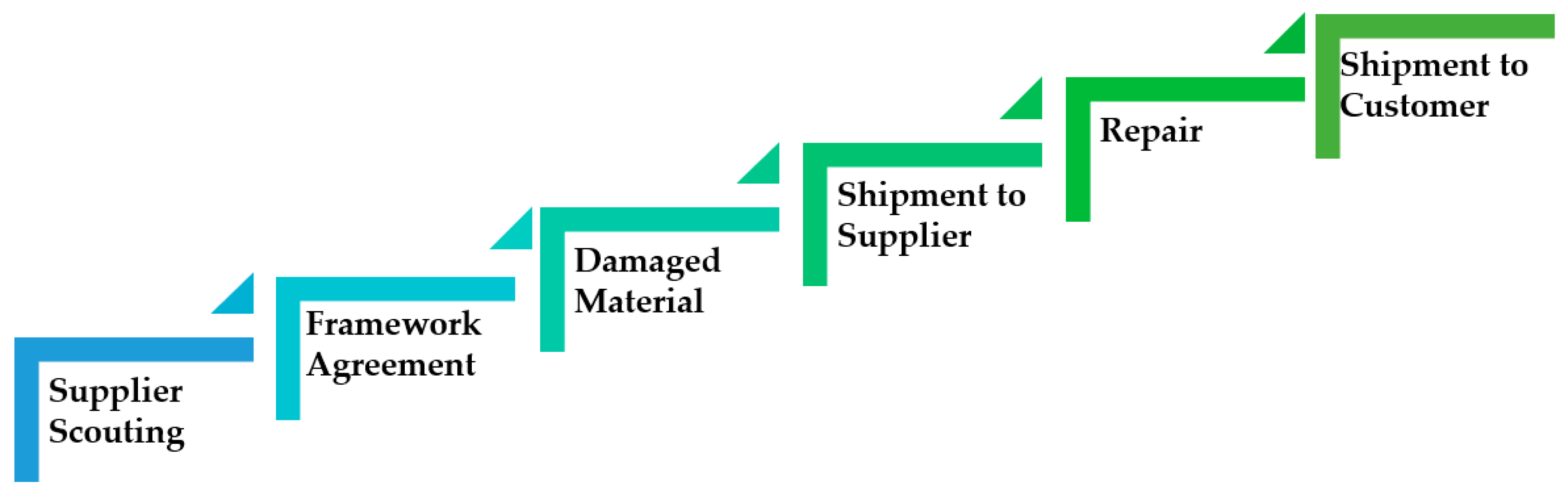
2.3. Full Service and Maintenance
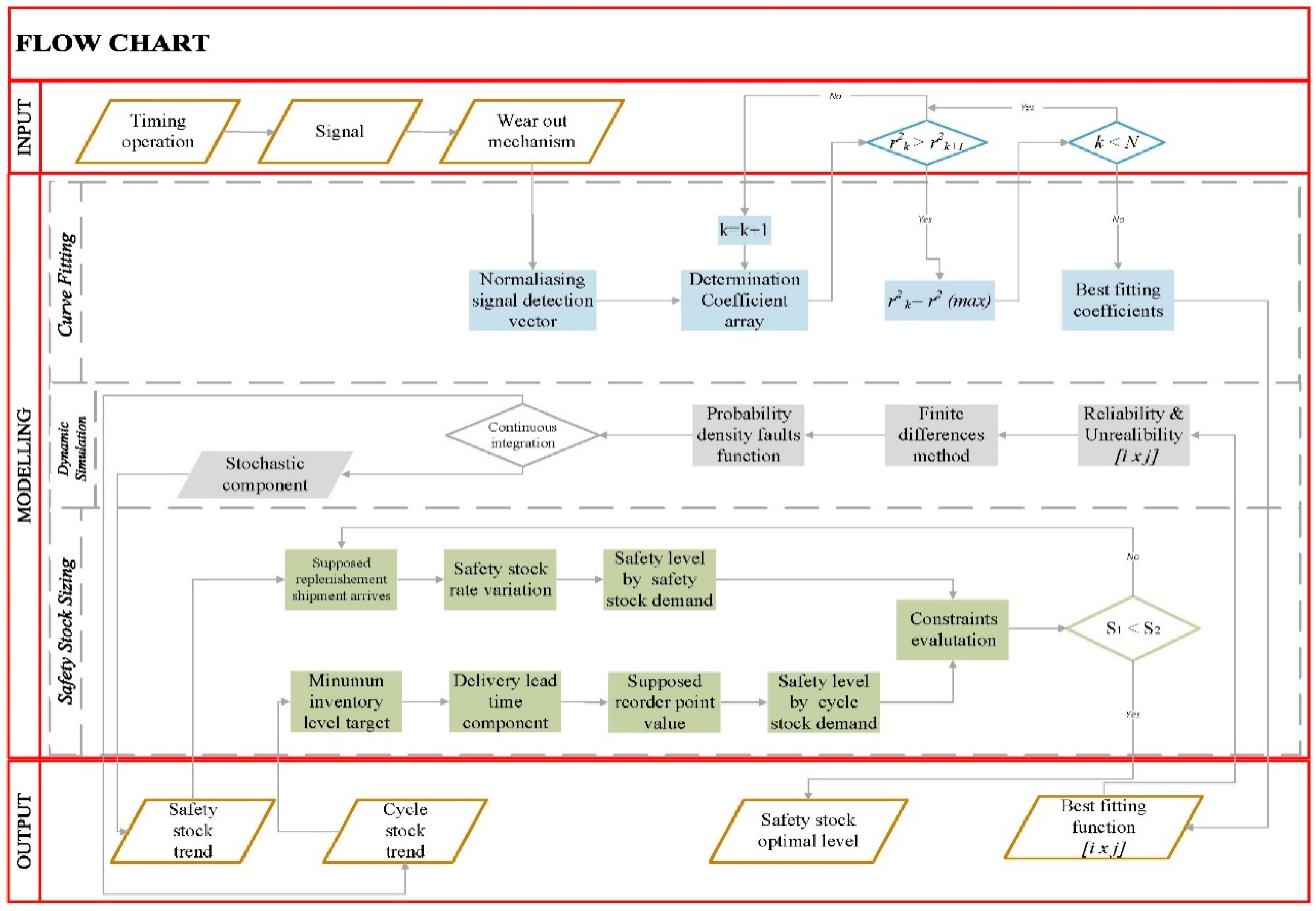
3. Proposed Methodology
3.1. Assumption and Notations
- the only variability is due to the failure rate;
- the items’ wear-out rate represents demand;
- each item has the maximum reliability value at the initial time;
- demand is a random variable;
- the supply is in equal lots;
- constant lead time.
- input
- ⚬
- timing operation detection, the time interval in which the item wear-out is recorded;
- ⚬
- signal operation detection, the item wear-out signal value;
- ⚬
- lead time;
- ⚬
- safety stock stochastic gain.
- output
- ⚬
- reliability functions;
- ⚬
- stock temporal trend;
- ⚬
- safety stock trend;
- ⚬
- optimal safety stock value.
- maximum inventory level, maximum stock can be stored, bound by stock availability:
- minimum inventory level, since it is a model in the absence of backorders, the stock value must never fall below a limit value, in this regard, the demand trend will be an end to a value equal to 5% of residual life:
- must never be less than 99.5%, thus constraining the percentile standard normal distribution value:
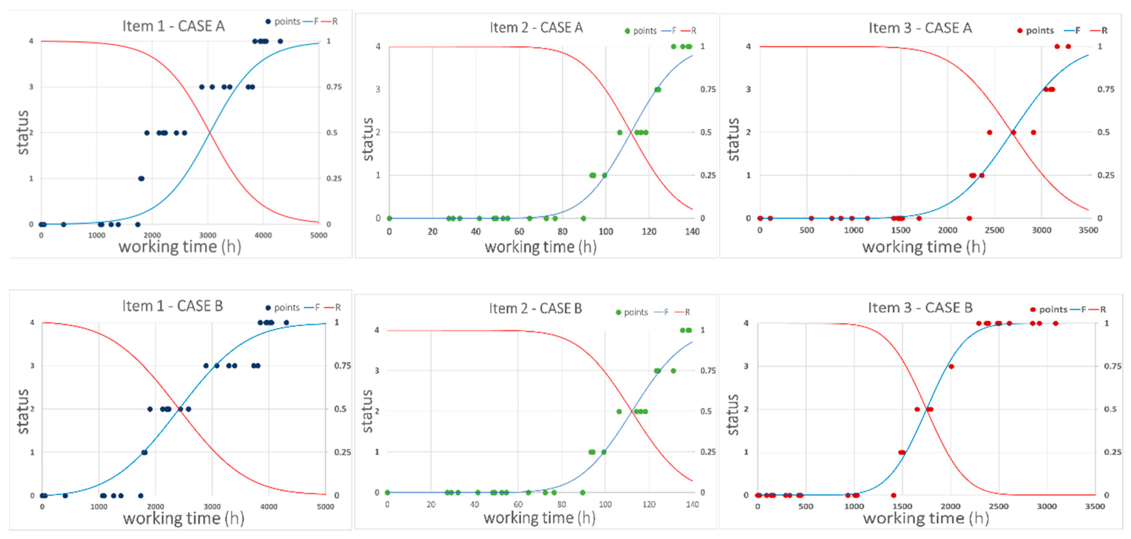
3.2. Reliability Rate Modeling as Stock Demand
- t = 0 => λ(0) = 0:
- t = T => λ(T) = λMAX:
3.3. Stochastic Safety Stock Gain
3.4. Wear-Out Related Safety Stock Gain
3.5. EOQ Dynamic Model Implementation
4. Case Study
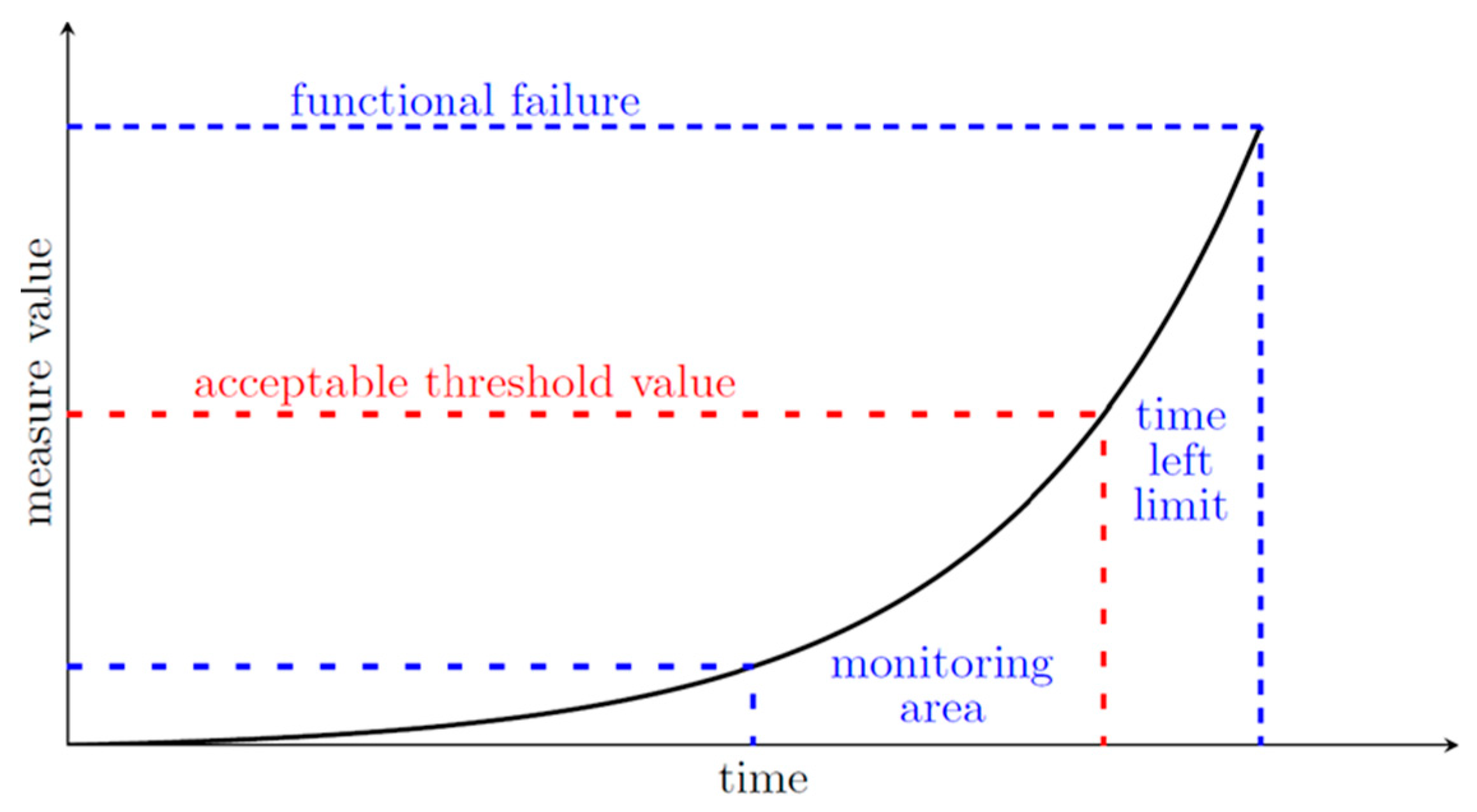
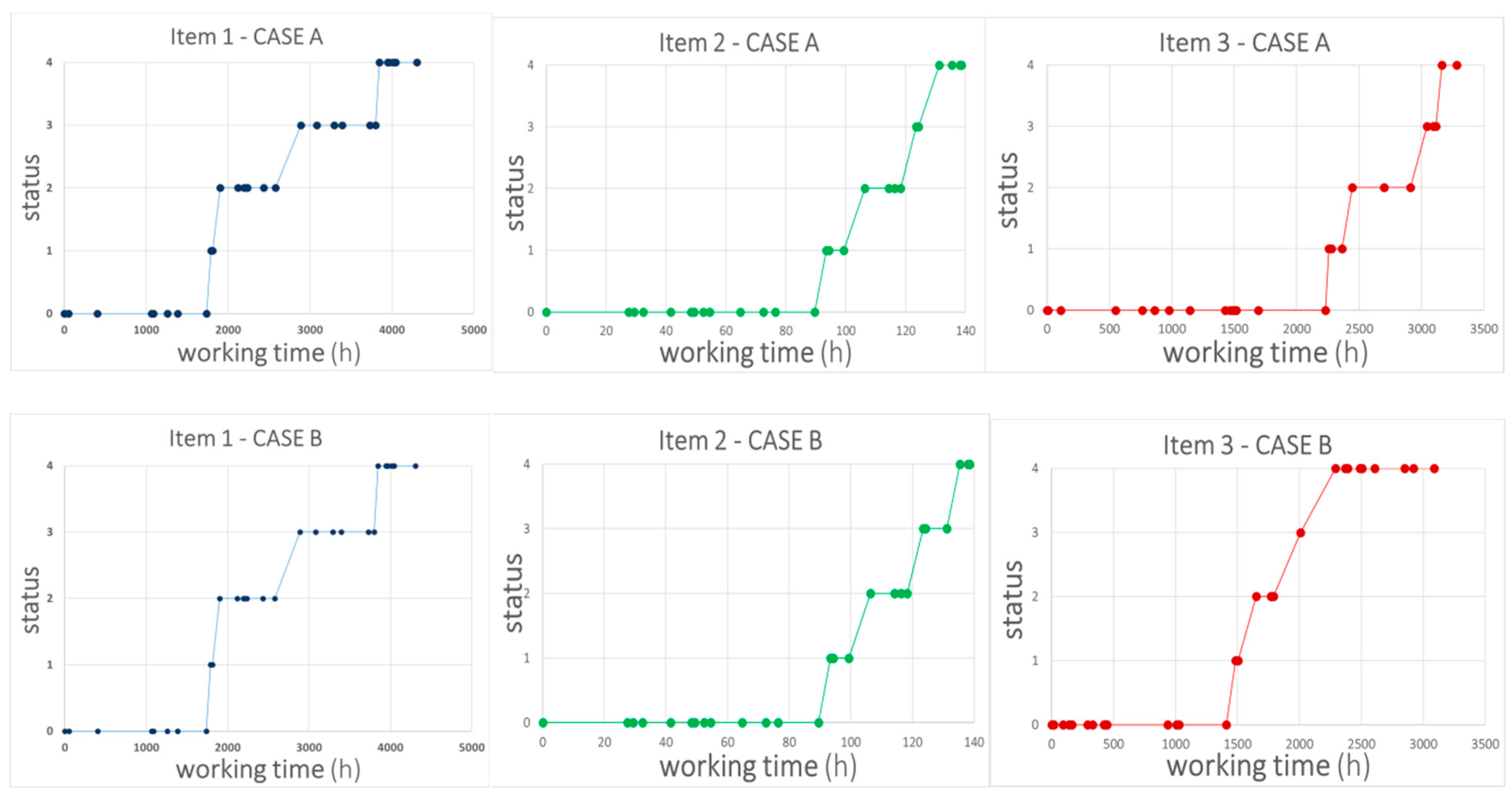
4.1. Wear-Out Rate Evaluation
- the advance of maintenance requirements before the actual fault occurrence;
- system reliability improvement through preventive maintenance;
- improvement in problem resolution times;
- improving the supply chain due to the status component clear definition.
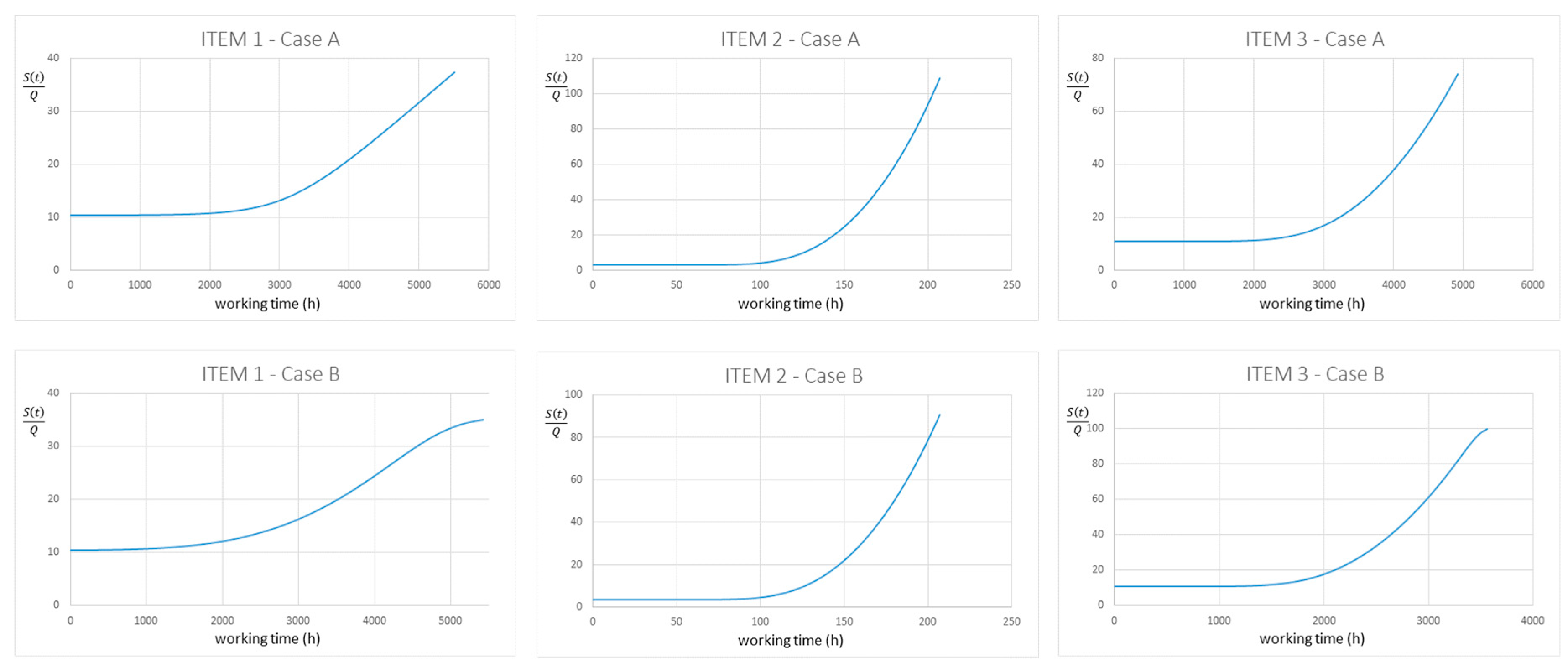
4.2. Safety Stock Sizing
4.2.1. Supply Chain Input Value
4.2.2. Safety Stock Contributions
5. Result Analysis
6. Conclusions
Author Contributions
Funding
Conflicts of Interest
Appendix A
References
- Courtois, A.; Martin-Bonnefous, C.; Pillet, M. Gestion de la Production; Editions d’Organisation: Paris, France, 2003; Chapter 3. [Google Scholar]
- Tang, C.S. Perspectives in supply chain risk management. Int. J. Prod. Econ. 2006, 103, 451–488. [Google Scholar] [CrossRef]
- Coculescu, C. Comparative Evaluation of Parametric Optimization Methods. Econ. Comput. Economic Cybern. Stud. Res. 2017, 41, 197. [Google Scholar]
- Santos, R.J.; Bernardino, J. Real-time data warehouse loading methodology. In Proceedings of the 2008 International Symposium on Database Engineering & Applications, Coimbra, Portuga, 10–12 September 2008. [Google Scholar]
- Calafiore, G.; Dabbene, F.; Tempo, R. Research on probabilistic methods for control system design. Automatica 2011, 47, 1279–1293. [Google Scholar] [CrossRef]
- Ruijters, E.; Stoelinga, M. Fault tree analysis: A survey of the state-of-the-art in modeling, analysis and tools. Comput. Sci. Rev. 2015, 15, 29–62. [Google Scholar] [CrossRef] [Green Version]
- Barlow, R.; Proschan, F. Statistical Theory of Reliability and Life Testing: Probability Models; Holt, Rinehart and Winston: Singapore, 1975. Available online: https://books.google.it/books?id=4DGm18gSnNcC&pg=PA105&lpg=PA105&dq=7.%09Barlow,+R.;+Proschan,+F.+Statistical+Theory+of+Reliability+and+Life+Testing:+Probability+Models;+Holt,+Rinehart+and+Winston:+1975&source=bl&ots=JAT03lyhe&sig=ACfU3U3r5JWgOFUoIJpiremOUkLhEjxtkA&hl=en&sa=X&ved=2ahUKEwiopfyd27HpAhVINOwKHaZ_ALUQ6AEwBnoECAcQAQ#v=onepage&q=7.%09Barlow%2C%20R.%3B%20Proschan%2C%20F.%20Statistical%20Theory%20of%20Reliability%20and%20Life%20Testing%3A%20Probability%20Models%3B%20Holt%2C%20Rinehart%20and%20Winston%3A%201975&f=false (accessed on 15 October 2019).
- Anders, G.J. Probability Concepts in Electric Power Systems; J. Wiley & Sons: New York, NY, USA, 1990. [Google Scholar]
- Ding, S.H.; Kamaruddin, S. Maintenance policy optimization—Literature review and directions. Int. J. Adv. Manuf. Technol. 2015, 76, 1263–1283. [Google Scholar] [CrossRef]
- Rastayesh, S.; Bahrebar, S.; Blaabjerg, F.; Zhou, D.; Wang, H.; Dalsgaard Sørensen, J. A System Engineering Approach Using FMEA and Bayesian Network for Risk Analysis—A Case Study. Sustainability 2020, 12, 77. [Google Scholar] [CrossRef] [Green Version]
- Zheng, R.; Su, C. A warranty policy for repairable products with bathtub-shape failure rate. In Proceedings of the Prognostics and System Health Management Conference, Chongqing, China, 26–28 October 2018. [Google Scholar]
- Berrade, M.D.; Cavalcante, C.A.V.; Scarf, P.A. Maintenance scheduling of a protection system subject to imperfect inspection and replacement. Eur. J. Oper. Res. 2012, 218, 716–725. [Google Scholar] [CrossRef]
- Barata, J.; Soares, C.G.; Marseguerra, M.; Zio, E. Simulation modelling of repairable multi-component deteriorating systems for “on condition” maintenance optimization. Reliab. Eng. Syst. Saf. 2002, 76, 164–225. [Google Scholar] [CrossRef]
- Jardine, A.K.; Lin, D.; Banjevic, D. A review on machinery diagnostics and prognostics implementing condition-based maintenance. Mech. Syst. Signal Process. 2006, 20, 1483–1510. [Google Scholar] [CrossRef]
- Bevilacqua, M.; Bottani, E.; Ciarapica, F.E.; Costantino, F.; Di Donato, L.; Ferraro, A.; Mazzuto, G.; Monteriù, A.; Nardini, G.; Ortenzi, M.; et al. Digital Twin Reference Model Development to PreventOperators’ Risk in ProcessPlants. Sustainability 2020, 12, 1088. [Google Scholar] [CrossRef] [Green Version]
- Modgil, S.; Sharma, S. Total productive maintenance, total quality management and operational performance. J. Qual. Maint. Eng. 2016, 22, 353–377. [Google Scholar] [CrossRef]
- Mwanza, B.G.; Mbohwa, C. Design of a Total Productive Maintenance Model for Effective Implementation: Case Study of a Chemical Manufacturing. Co. Procedia Manuf. 2015, 4, 461–470. [Google Scholar] [CrossRef] [Green Version]
- De Felice, F.; Petrillo, A. An overview on human error analysis and reliability assessment. In Human Factors and Reliability Engineering for Safety and Security in Critical Infrastructures. Decision Making, Theory, and Practice; Series in Reliability Engineering; Springer: Naples, FL, USA, 2018; pp. 19–41. [Google Scholar]
- Stremersch, S.; Wuyts, S.; Frambach, R.T. The Purchasing of Full-Service Contracts: An Exploratory Study within the Industrial Maintenance Market. Ind. Mark. Manag. 2001, 30, 1–12. [Google Scholar] [CrossRef]
- Vandermerwe, S.; Rada, J. Servitization of Business: Adding Value by Adding Services. Eur. Manag. J. 1988, 6, 314–324. [Google Scholar] [CrossRef]
- Glenn, E.; Kovalova, E.; Machova, V.; Konecny, V. Big Data Analytics Processes in Industrial Internet of Things Systems: Sensing and Computing Technologies, Machine Learning Techniques, and Autonomous DecisionMaking Algorithms. J. Self-Gov. Manag. Econ. 2019, 7, 28–34. [Google Scholar]
- Zhuravleva, N.A.; Nica, E.; Durana, P. Sustainable Smart Cities: Networked Digital Technologies, Cognitive Big Data Analytics, and Information Technology-driven Economy. Geopolit. Hist. Int. Relat. 2019, 11, 41–47. [Google Scholar]
- Putnam Dermot Kovacova, M.; Valaskova, K.; Stehel, V. The Algorithmic Governance of Smart Mobility: Regulatory Mechanisms for Driverless Vehicle Technologies and Networked Automated Transport Systems. Contemp. Read. Law Soc. Justice 2019, 11, 21–26. [Google Scholar]
- Porter, M.E. Location, Competition, and Economic Development: Local Clusters in a Global Economy. Econ. Dev. Q. 2000, 14, 15–34. [Google Scholar] [CrossRef]
- Petrillo, A.; De Felice, F.; Cioffi, R.; Zomparell, F. Fourth Industrial Revolution: Current Practices, Challenges, and Opportunities. In Digital Transformation in Smart Manufacturing; TECH Publisher: New Delhi, India, 2018. [Google Scholar]
- Yadav, A.S.; Gupta, K.; Garg, A.; Swami, A. A two warehouse inventory models for deteriorating items with shortages under genetic algorithm and PSO. Int. J. Emerg. Trends Technol. Comput. Sci. 2015, 4, 40–48. [Google Scholar]
- Chopra, S.; Meindl, P. Supply Chain Management: Strategy, Planning, and Operation, 6th ed.; Pearson: London, UK, 2016. [Google Scholar]
- De Felice, F.; Petrillo, A.; Zomparelli, F. Prospective design of smart manufacturing: An Italian pilot case study. Manuf. Lett. 2018, 15, 81–85. [Google Scholar] [CrossRef]
- Facchini, F.; Oleskow-Szlapka, J.; Ranieri, L.; Urbinati, A. A Maturity Model for Logistics 4.0: An Empirical Analysis and a Roadmap for Future Research. Sustainability 2020, 12, 86. [Google Scholar] [CrossRef] [Green Version]
- Inderfurth, K.; Minner, S. Safety stocks in multistage inventory systems under different service measures. Eur. J. Oper. Res. 1998, 106, 57–73. [Google Scholar] [CrossRef]
- Rambau, J.; Schade, K. The Stochastic Guaranteed Service Model with Recourse for Multi-Echelon Warehouse Management. Electron. Notes Discret. Math. 2010, 36, 783–790. [Google Scholar] [CrossRef] [Green Version]
- Klosterhalfen, S.T.; Dittmar, D.; Minner, S. An integrated guaranteed and stochastic service approach to inventory optimization in supply chain. Eur. J. Oper. Res. 2013, 231, 109–119. [Google Scholar] [CrossRef]
- Moncayo-Martínez, L.A.; Reséndiz-Flores, E.O.; Mercado, D.; Sánchez-Ramírez, C. Placing Safety Stock in Logistic Networks under Guaranteed-Service Time Inventory Models: An Application to the Automotive Industry. J. Appl. Res. Technol. 2014, 12, 538–550. [Google Scholar] [CrossRef]
- Chen, H.; Li, P. Optimization of (R,Q) policies for several inventory system using the guaranteed service approach. Comput. Ind. Eng. 2015, 80, 261–273. [Google Scholar] [CrossRef]
- Lohnert, M.; Rambau, J. Modeling Demand Propagation in Guaranteed Service Models. Int. Fed. Autom. Control 2018, 51, 284–289. [Google Scholar]
- De Kok, T.; Grob, C.; Laumanns, M.; Minner, S.; Rambau, J.; Schade, K. A typology and literature review on stochastic multi-echelon inventory models. Eur. J. Oper. Res. 2018, 269, 955–983. [Google Scholar] [CrossRef] [Green Version]
- Puga, M.S.; Minner, S.; Tancrez, J.S. Two stage supply chain design with safety stock placement decision. Int. J. Prod. Econ. 2019, 209, 183–193. [Google Scholar] [CrossRef] [Green Version]
- Plebankiewicz, E.; Meszek, W.; Zima, K.; Wieczorek, D. Probabilistic and Fuzzy Approaches for Estimating the Life Cycle Costs of Buildings under Conditions of Exposure to Risk. Sustainability 2020, 12, 226. [Google Scholar] [CrossRef] [Green Version]
- Birkel, H.S.; Veile, J.W.; Müller, J.M.; Hartmann, E.; Voigt, K.-I. Development of a Risk Framework for Industry 4.0 in the Context of Sustainability for Established Manufacturers. Sustainability 2019, 11, 384. [Google Scholar] [CrossRef] [Green Version]


| Signal Detection | Criteria | Operating State | Priority |
|---|---|---|---|
| 0 | No deviation | Normal State |  |
| 1 | A deviation more significant than the nominal operating state was detected five times | The component has an initial degradation. The behavior must be closely monitored. | |
| 2 | A deviation more significant than the nominal operating state was detected ten times | The component has an initial degradation. The revision must be planned. | |
| 3 | A deviation more significant than the nominal operating state was detected 15 times | The component has a degradation. The revision must be planned. | |
| 4 | A deviation more significant than the nominal operating state was detected 20 times | The component is a failure risk. The replacement must be planned. |
| Sigmoid Functions | Determination Coefficients | |||||
| ITEM 1 | ITEM 2 | ITEM 3 | ||||
| Case A | Case B | Case A | Case B | Case A | Case B | |
| Logistic | 0.8864 | 0.9239 | 0.9653 | 0.9659 | 0.9461 | 0.9903 |
| Three-parameter Weibull | 0.5497 | 0.3223 | 0.5063 | 0.5151 | 0.1650 | 0.3534 |
| Arctangent | 0.8809 | 0.9152 | 0.9654 | 0.9592 | 0.9393 | 0.9570 |
| Gudermannian | 0.1603 | 0.1467 | 0.5368 | 0.5277 | 0.1453 | 0.1974 |
| Error | 0.0132 | 0.9278 | 0.9684 | 0.9686 | 0.9478 | 0.9915 |
| Algebraic | 0.7865 | 0.8257 | 0.7139 | 0.7271 | 0.6571 | 0.7657 |
| Modular | 0.6867 | 0.6977 | 0.6010 | 0.6156 | 0.5452 | 0.6461 |
| Functions Parameters | ||||||
| Best Fitting Function | Logistic | Error | Error | Error | Error | Error |
| A value | −0.0023 | 0.07512 | 0.4040 | 0.0373 | 0.0014 | 0.0022 |
| B Value | 6.8534 | −1.8043 | −4.5066 | −4.1874 | -3.8466 | −3.9299 |
| Analytical Form | CASE A | CASE B |
|---|---|---|
| ITEM 1 | ||
| ITEM 2 | ||
| ITEM 3 |
| Lead Time (h) | Extra lead Time (h) | Replacement for Electrical/Mechanical Failure | Replacement for Other Reasons | Total Exits Movements | Percentage of Exit Due to Failure | |
|---|---|---|---|---|---|---|
| ITEM 1 | 320 | 30 | 9 | 0 | 9 | 100% |
| ITEM 2 | 30 | 0 | 64 | 3 | 67 | 95.52% |
| ITEM 3 | 250 | 0 | 8 | 3 | 11 | 72.73% |
| α | 0.995 | 0.997 | 0.999 | ||
|---|---|---|---|---|---|
| z | 2.12 | 2.37 | 2.71 | ||
| ITEM 1 | 0.2144 | 8.14 | 9.10 | 10.40 | |
| ITEM 2 | 0.1873 | 2.51 | 2.80 | 3.21 | |
| ITEM 3 | 0.2253 | 8.54 | 9.55 | 10.92 | |
| ITEM 1 | ITEM 2 | ITEM 3 | ||||
|---|---|---|---|---|---|---|
| Case A | Case B | Case A | Case B | Case A | Case B | |
| 10.38 | 9.75 | 28.85 | 34.45 | 14.07 | 21.47 | |
| 14.77 | 13.50 | 33.71 | 36.19 | 20.42 | 28.71 | |
| 19.32 | 18.19 | 45.73 | 44.32 | 24.34 | 30.34 | |
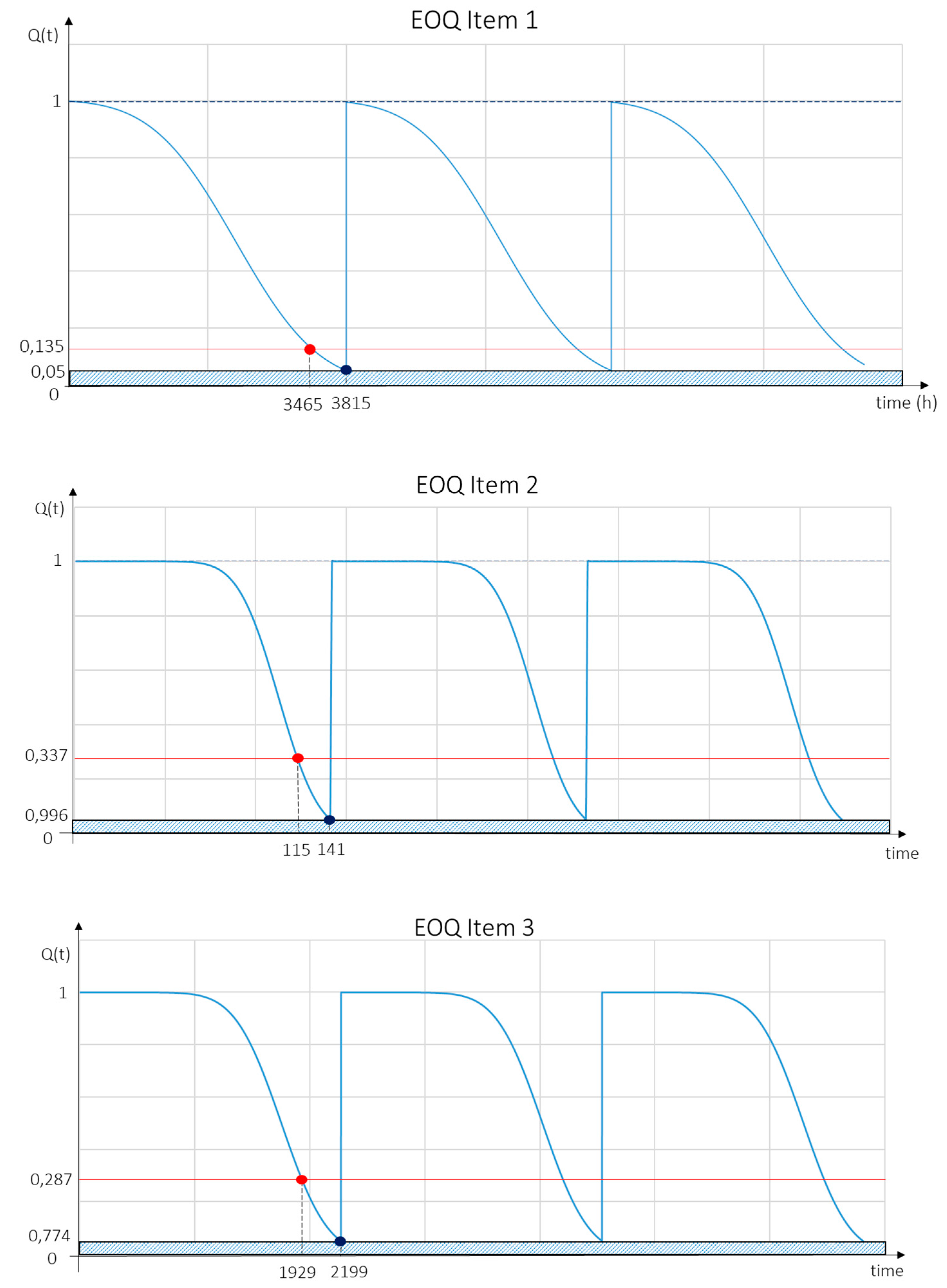
| Reorder Point (h) | 3816 | 3465 | 115 | 117 | 3092 | 1929 |
| Inbound (h) | 4166 | 3815 | 145 | 147 | 3372 | 2199 |
| Inbound remaining stock | 6.90% | 6.67% | 9.96% | 10.43% | 8.14% | 7.74% |
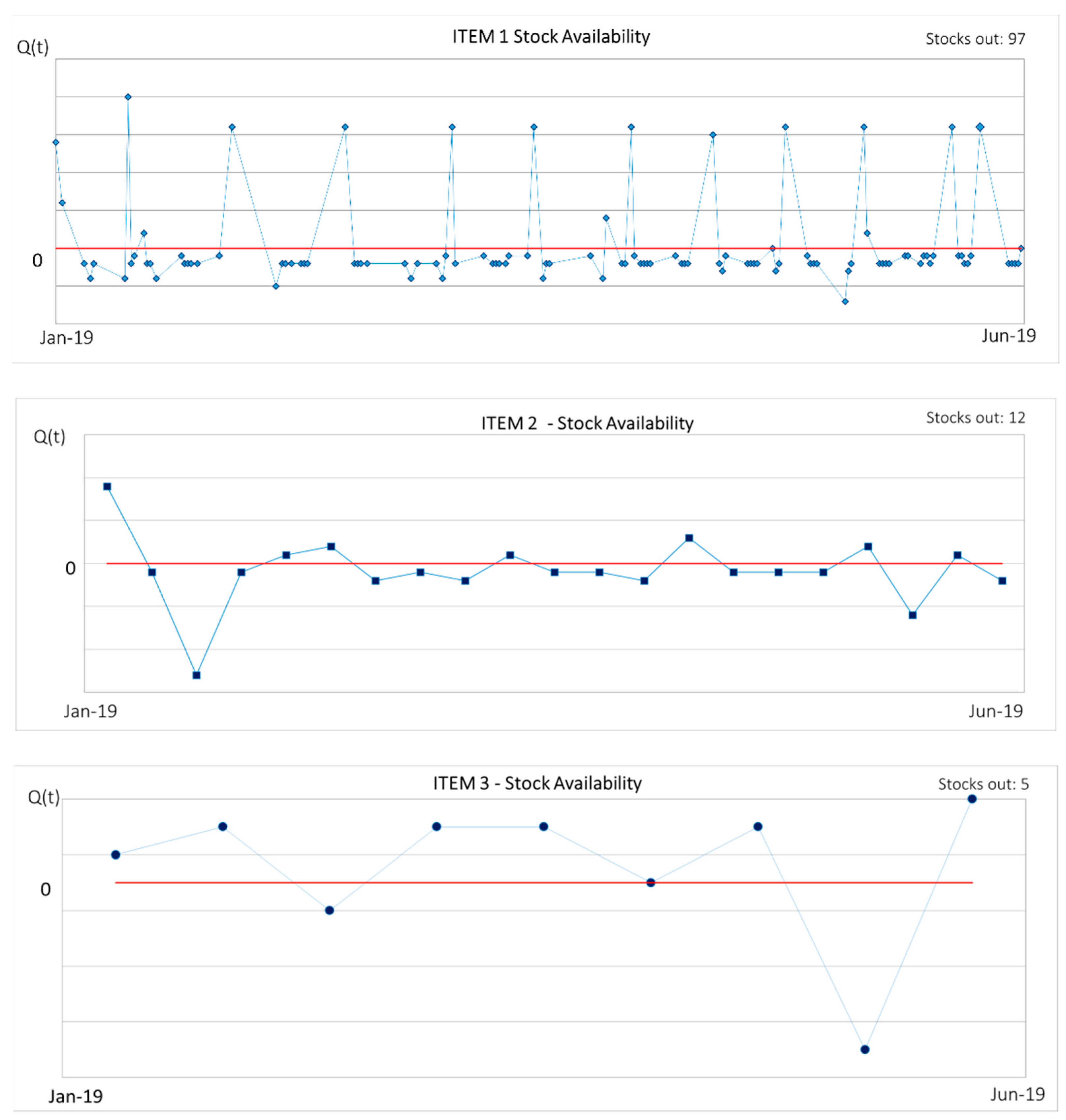
| Stock-out Events | |
|---|---|
| ITEM 1 | 97 |
| ITEM 2 | 12 |
| ITEM 3 | 5 |
© 2020 by the authors. Licensee MDPI, Basel, Switzerland. This article is an open access article distributed under the terms and conditions of the Creative Commons Attribution (CC BY) license (http://creativecommons.org/licenses/by/4.0/).
Share and Cite
Di Nardo, M.; Clericuzio, M.; Murino, T.; Sepe, C. An Economic Order Quantity Stochastic Dynamic Optimization Model in a Logistic 4.0 Environment. Sustainability 2020, 12, 4075. https://doi.org/10.3390/su12104075
Di Nardo M, Clericuzio M, Murino T, Sepe C. An Economic Order Quantity Stochastic Dynamic Optimization Model in a Logistic 4.0 Environment. Sustainability. 2020; 12(10):4075. https://doi.org/10.3390/su12104075
Chicago/Turabian StyleDi Nardo, Mario, Mariano Clericuzio, Teresa Murino, and Chiara Sepe. 2020. "An Economic Order Quantity Stochastic Dynamic Optimization Model in a Logistic 4.0 Environment" Sustainability 12, no. 10: 4075. https://doi.org/10.3390/su12104075