Article

The Combined Distribution and Assignment Model: A New Solution Algorithm and Its Applications in Travel Demand Forecasting for Modern Urban Transportation

1
College of Civil and Transportation Engineering, Hohai University, 1 Xikang Road, Nanjing 210098, China
2
School of Business, Jinling Institute Technology, Nanjing 211100, China
3
Road Traffic Safety Research Center of Ministry of Public Security, Beijing 100062, China
*
Author to whom correspondence should be addressed.
Sustainability 2019, 11(7), 2167; https://doi.org/10.3390/su11072167
Submission received: 7 March 2019 / Revised: 28 March 2019 / Accepted: 9 April 2019 / Published: 11 April 2019
(This article belongs to the Special Issue Sustainable and Intelligent Transportation Systems)

Abstract

:
With the development of the advanced Intelligent Transportation System (ITS) in modern cities, it is of great significance to upgrade the forecasting methods for travel demand with the impact of ITS. The widespread use of ITS clearly changes the urban travelers’ behavior at present, in which case it is difficult for the conventional four-step travel demand forecasting model to have good performance. In this study, we apply the combined distribution and assignment (CDA) model to forecasting travel demand for modern urban transportation, in which travelers may choose the destination and path simultaneously. Furthermore, we present a new solution algorithm for solving the CDA model. With the network representation method that converts the CDA model into a standard traffic assignment problem (TAP), we develop a new path-based algorithm based on the gradient projection (GP) algorithm to solve the converted CDA model. The new solution algorithm is designed to find a more accurate solution compared with the widely used algorithm, the Evans’ two-stage algorithm. Two road networks, Sioux Falls and Chicago Sketch, are used to verify the performance of the new algorithm. Also, we conduct some experiments on the Sioux Falls network to illustrate several applications of the CDA model in consideration of the influences of ITS.

1. Introduction

The advanced Intelligent Transportation System (ITS) has been adopted increasingly in many cities. In simple words, the system aims to enable users to be better informed and make safer, more coordinated, and “smarter” use of transportation networks by using some information and communication technologies, which can increase efficiency and reduce risks in the transportation systems of cities [1,2].
An accurate travel demand forecasting result is greatly significant for modern transportation, taking into consideration the impact of ITS (especially the travel demand distribution between traffic zones and the network flow pattern). ITS can be regarded as a platform to achieve different goals. For example, one reason why the ITS is designed is to provide some technical support for solving the problem of traffic congestion, which will lead to a series of problems (for instance, time losses, direct negative economic effects, air pollution, etc.) and has become one of the most intractable issues in modern cities. A promising approach to solve the traffic congestion problem is to redistribute the travel demand in space or in time, called travel demand management (TDM). ITS provides practical and essential technical support for many TDM strategies, such as detecting whether a car enters a congested areas in the implementation of a congestion pricing strategy. Moreover, travelers should be aware of the charge level of the congested areas in advance, so that they can make wiser decisions about their trips, which is also important for a congestion pricing strategy to be more effective. This information needs be accurate and in real time, which can be provided by ITS. To improve the efficiency of the transportation network, it is significant to have a good knowledge of the effects that the strategies will have on travelers’ behavior and the network flow, which means that an accurate travel demand forecasting result is necessary.
With the spread of ITS, it could be difficult for the traditional four-step travel demand forecasting model [3] (or the four-step model for short) to have good performance in predicting travel demand. That is because, on the one hand, with the rapid development of the economy, there are more commercial centers and entertainment facilities in the urban area, which means that there are more alternative destination choices for non-working (shopping and recreating) trips for travelers; on the other hand, with the help of ITS, travelers have access to more detailed and accurate traffic information (for example, information about trip cost, parking fees, and congestion conditions at the destination area). This information has significant impacts on the travelers’ destination choice behavior. Considering the situation in which travelers think that the parking fee or the trip cost is too high due to the traffic congestion, they may want to change their original trip destinations to alternative zones. This indicates that travelers may consider the destination choice step and the path choice step simultaneously, which differs from the assumptions of the conventional four-step model (i.e., travelers will consider their trip in a sequential order, deciding the trip’s destination first, and then choose the trip path).
Fortunately, the travelers’ behavior described in the above is consistent with the combined distribution and assignment (CDA) model, which has been widely studied in the literature. Tomlin first proposed the CDA model based on the entropy-type model [4]. Florian et al. proposed a CDA model with destination demand function [5]. Evans developed a widely used algorithm (i.e., the two-stage algorithm) to solve the CDA model [6]. Oppenheim proposed a CDA model with variable destination costs [7] and Yao et al. put forward a general unconstrained optimization model for the CDA problem [8].
Also, the CDA model has been applied to solve many practical problems in recent years. Yang et al. proposed a bi-level model, in which the lower-level model is the CDA model, to solve the network capacity and level of service problem [9]. This model has also been exploited to estimate the capacity of urban transportation networks with rapid transit [10] and identify critical links in road networks [11]. Chen et al. presented network-based accessibility measures for assessing vulnerability of degradable transportation networks based on the CDA model [12]. Besides, Chen et al. employed the CDA model to measure capacity flexibility [13] and estimate capacity reliability [14] of transportation networks. Moreover, Yim et al. used the CDA model to map the land-use pattern to the link-loading pattern in the network for the land use problems [15].
In this paper, the CDA model is adopted to forecast travel traffic demand for urban transportation with the impacts of ITS. Only the singly-constrained CDA model is considered because the trip production of each traffic zone is relatively fixed (it is not likely for travelers to often change their residences) and the data can be rather easy to get. In order to show some applications of the CDA model in ITS, we also conduct several experiments by examining: (1) differences in network flow pattern between the four-step and CDA model; (2) effects of multiple commercial centers on travelers’ behavior; (3) application of the CDA model to two TDM strategies, namely the parking charge and congestion charge strategy.
In addition, we notice that with the widely used algorithm, Evans’ two-stage algorithm [6], it is difficult to achieve relatively high precision, which is required in the process of forecasting travel demand (for example, for consistent comparison between design scenarios [16]). This inferiority may result from the iterative equilibration between the origin and destination (O–D) flow and network flow. An alternative method for solving the CDA model is referred to as the network representation method, presented by Sheffi [17]. It converts the CDA model to a standard traffic assignment problem (TAP) by adding dummy destinations and links to the original network, and then solves the converted CDA model with convergent TAP algorithms. The network representation method avoids solving the trip distribution step and traffic assignment step iteratively, which means it may obtain a high-precision solution.
The gradient projection (GP) method proposed by Jayakrishnan et al. [18], a type of path-based algorithm, has shown a successful performance in solving the TAP. Recently, the GP method has been applied to various network equilibrium problems: the logit-based SUE model [19,20], the non-additive traffic equilibrium problem [21], the elastic-demand traffic equilibrium problem (EDTEP) [22], etc. Furthermore, the GP method has also been applied to one of the combined models, the combined modal split and traffic assignment model (CMSTA) [23].
However, the original GP method is inefficient in solving the converted CDA problem because there are a large number of paths between each O–D pair in the converted problem. The flow transferring scheme in this method is that flows are shifted from the non-shortest paths to the shortest one between each O–D pair. When there are plenty of paths existing between each O–D pair, the scheme could restrict the algorithm from obtaining high efficiency in solving the TAP. To overcome this problem, we develop a new flow transferring strategy inspired by the GP method to improve the algorithm’s efficiency and accuracy. Our numerical results show that the network representation method incorporated with the new flow transferring strategy outperforms the widely used two-stage algorithm.
The contributions of this paper are twofold. On the one hand, with the network representation method converting the CDA model into a standard TAP, we develop a new path-based algorithm inspired by the GP algorithm to solve the converted CDA model. Compared with the widely used algorithm (the two-stage algorithm), the new algorithm can achieve a solution with higher precision. On the other hand, considering the impacts of ITS, we adopt the CDA model to forecast travel demand for modern urban transportation. The CDA model has a better interpretation of travelers’ behavior, because travelers may decide the destination and route simultaneously with access to more detailed and accurate trip information.
The rest of this paper is organized as follows. Section 2 describes the CDA model and two solution methods—the widely used two-stage method and the network representation method. Section 3 briefly reviews the gradient projection algorithm and presents a new multiple path gradient projection algorithm. Section 4 provides several numerical experiments to examine: (1) the comparison between the two-stage algorithm and the proposed algorithm for solving the CDA model; and (2) several applications of the CDA model. Finally, some conclusions are provided in Section 5.

2. Mathematical Programming Formulation

2.1. Singly Constrained CDA Model

To incorporate the rapid development of urban areas and the help of ITS, in which there are more alternative trip destination choices and detailed traffic information for travelers, the CDA model is suggested. Furthermore, since the trip production in each zone is relatively fixed and the data is easier to obtain, the singly constrained CDA model (with trip production constraints at origins only) is more suitable than the doubly constrained CDA model (with both trip production constraints at origins and trip attraction constraints at destinations).
Sheffi developed a CDA model in which the attractiveness of each destination is constant [17], and Oppenheim modified the CDA model with variable destination cost, which is a function with respect to the trip attraction of the corresponding destination [7]. In fact, there are many factors influencing people’s travel behavior when travelers have access to more detailed traffic information with ITS. Some of them may be fixed (such as how attractive the entertainment facilities are to travelers), while the others are related to the trip attraction of each destination (such as the congestion level). Hence, the CDA model with variable destination cost proposed in a previous study [7] is more suitable to handle this situation. In addition, in order to apply the network representation method illustrated by Sheffi [17] to solving this model, we rewrite the CDA model developed by Oppenheim [7]. The CDA model used in this paper is shown in the following (“the CDA model” refers to only the singly-constrained CDA model for the remainder of this paper).
Consider a directed transportation network G(N, A), where N and A denote the sets of nodes and links, respectively. Suppose that there is at least one path between any two nodes in G. Let R N be the origin set, and S N be the destinations set. A link, connecting two nodes, is denoted by a. Let va be the flow through link a, and the cost of link a is denoted by ta, which is a monotone increasing function with respect to va. Let qrs and urs denote the travel demand and the travel cost from origin r to destination s, respectively. The trip production of origin r is denoted by Or. Let Krs be the set of simple paths between rs, and fk be the flow on path k Krs. The constant attraction measure term of destination s, which is irrelevant to the total number of trips ending at s, is denoted as Ms. The variable destination cost term at s, denoted as w s , is a function that is either all increasing or all decreasing in the trip production of destination s (i.e., r R q r s ), which reflects either negative or positive externalities generated by traffic.
The CDA model in this study is based on the following assumptions:
(a) The trip production at each origin, r, is fixed, but trip attraction at each destination is not, i.e., is singly-constrained, which is given by:
s S q r s = O r ,   r R
(b) The trip production constraint (Equation (1)) is satisfied by using a multinomial logit model, which is formulated as the following destination demand function:
v r s = O r e γ ( u r s M s + w s ) m S e γ ( u r m M m + w s ) ,   r R ,   s S
where γ and M s are assumed to be parameters and can be estimated from observations regarding travelers’ choices of destination; w s is a function that is either all increasing or all decreasing in the trip attraction at destination s; ursMs + w s can be regarded as the net travel cost.
(c) At equilibrium, the travel cost on all paths with positive flow between each O–D pair will be equal and no greater than the travel cost on any unused paths.
Based on the above assumptions, the CDA problem can be mathematically formulated as follows:
m i n z ( x , q ) = a A 0 x a t a ( y ) d y + r R ,   s S [ 1 γ ( q r s l n q r s q r s ) M s q r s ] + s S 0 r R q r s w s ( y ) d y
subject to:
k K r s f k = q r s ,   r R ,   s S
s S q r s = O r ,   r R  
f k     0 ,   k K r s ,   r R ,   s S
q r s 0 ,   r R ,   s S
x a = r R s S k K r s f k δ a , k r s ,   a A
where δ a , p r s is a link/path indicator, which equals 1 if link a is on path k K r s , and 0 otherwise; γ is the parameter of the multinomial logit model; ta(x) is the cost function of link a.
It can be easily verified that the Karush-Kuhn-Tucker (KKT) condition of the above model is equivalent to the multinomial logit-based share model of Equation (2). Based on previous studies [7,17], as long as the destination functions are either all increasing or all decreasing in the destination volume, it is not difficult to prove that the equilibrium always exists and is always unique in terms of O–D flows.

2.2. Two-Stage Method

The most widely used method to solve the CDA problem is the two-stage method, proposed by Evans [6]. This method separates the CDA model into two sub-problems, trip distribution and traffic assignment, and solves the sub-problems iteratively. For each iteration of the two-stage method, firstly, auxiliary O–D travel demands are calculated by the logit model with the current shortest path cost as the O–D travel cost; secondly, the new O–D demand solution is obtained by the convex combination of the current travel demand solution and the auxiliary travel demand solution (the line search scheme is exploited). The above procedure intends to solve the trip distribution problem, and the result is the demand between each O–D pair. With the O–D demand being fixed, the problem is reduced to a TAP, which can be solved easily. The two-stage method solves the CDA problem by executing the procedures iteratively. This method for the CDA problem is easily implemented and straightforward, but it has difficulties in reaching high precision due to the iterative equilibration between the O–D flow and network flow (this inferior will be shown in the numerical experiment results).

2.3. Network Representation Method

As an alternative to the two-stage method, the network representation method can convert the CDA problem to a TAP by adding certain nodes and links. A simple augmented network explains the required modifications to solve the CDA model presented in the above, which is shown in Figure 1. Some explanations may be helpful to understand the augmentation. There are two origins (r and p) and three destinations (1, 2, and 3) in the basic network. Each origin or destination node is associated with a dummy origin or destination node in the dummy network. Accordingly, there are two dummy origins (r′ and p′) and three dummy destinations (1′, 2′, and 3′) in Figure 1. The network is augmented by dummy links leading from each actual destination (1, 2, and 3) to the corresponding dummy destination (1′, 2′, and 3′) and from each dummy destination to each dummy origin (r′ and p′). The flow from an actual destination to the corresponding dummy destination is equal to the trip attraction at the destination (for example, the flow on the dummy link, 1→1′, is equal to qr1+ qp1 in Figure 1). The flow from each dummy destination to each dummy origin is equal to the travel demand between the corresponding O–D pair (such as, the flow on the dummy link, 1′→r′, is equal to qr1 in Figure 1).
Note that l i m b 0 + q r s l n q r s = 0, and therefore q r s l n q r s , can be assumed to be zero for q r s = 0. Consequently, the objective function in Equation (3) can be rewritten as follows:
m i n z ( x , q ) = a A 0 x a t a ( y ) d y + s S 0 r R q r s w s ( y ) d y + r R ,   s S 0 q r s ( 1 γ l n q r s M s ) d y
In the augmented network, the equivalent travel time on each dummy link leading from each actual destination to the corresponding dummy destination, ss′ (e.g., 1→1′), is w s , and the travel time on each dummy link from each dummy destination to the corresponding dummy origin, s′→r′ (e.g., 1′→r′), is ( 1 γ l n q r s M s ) . Hence, the second term and third term in Equation (9) can be regarded as the sum of the integrals of the cost functions on all dummy links. What is more, the flow on the link from origin r to the corresponding dummy node r′ is the trip production of origin r, which is fixed. Consequently, the CDA model is converted into a standard TAP with fixed demand in the modified network, in which the trips originating at r no longer end at each actual destination but at the corresponding dummy node r′.
It can be seen from the above that the core of two-stage method and network representation method is the TAP. The TAP in the two-stage method is easy to solve. However, there are some challenges to solving the TAP in the problem converted by the network representation method. This is because there are numerous paths between each O–D pair in this converted TAP, especially when there are lots of O–D pairs in the transportation network. The focus of the next section is on developing schemes to overcome this challenge.

3. A New Algorithm to Solve the CDA Problem

In this section, we first briefly review the GP method, which has been shown to be a successful algorithm to solve the TAP. Secondly, inspired by the GP algorithm, we focus on the new flow transferring scheme, which aims to improve the efficiency of solving the TAP with numerous paths between each O–D pair. At last, we introduce a new approach that incorporates the network representation method with the developed flow transferring scheme to solve the CDA model, and provide detailed procedures of the new algorithm for those who are interested in implementing it.

3.1. A Brief Review of the Gradient Projection Method

Jayakrishnan et al. [18] adopted the GP algorithm to solve the TAP in transportation networks. As a type of path-based algorithm, the GP algorithm exploits the O–D pair separability and separates the TAP into several sub-problems, in which only one pair of O–D is involved. For each sub-problem, under the demand conservation constraint, the shortest path flow can be expressed by the terms of the other path flows. Consequently, the TAP is redefined and there are only the non-negative constraints in the new problem. After that, a better solution can be searched by moving in the negative direction. Once an infeasible solution is reached, a projection is made to the constraint boundaries. Because of the redefinition of the problem, infeasibility occurs only when a variable violates the non-negative constraint, and thus the infeasible solution can be projected to the feasible region easily by making that variable zero. As a result, at a feasible solution, a new solution is calculated by:
f k = f k m i n { α c k c k ¯ a A k , k ¯ t a x a , f k } k k r s   k k ¯
f k ¯ = q r s k k r s , k k ¯ f k
where k ¯ denotes the shortest path in path set Krs; c k denotes the cost of path k; A k , k ¯ is the set of links that belong either to path k or to path k ¯ but not to both of them, and α is a predefined step size.
The gradient projection method has been shown to be a successful path-based algorithm for solving the user equilibrium TAP. However, due to the flow transferring scheme of shifting flows from each non-shortest path to the shortest one in the GP algorithm, it may be inefficient to handle the situation where there is a large number of paths in the used path set for each O–D pair, which is a significant feature of the converted CDA problem. Thus, we develop a flow transferring strategy to deal with this issue.

3.2. A New Flow Transferring Scheme to Solve the TAP

We develop a new flow transferring scheme, called a multi-path gradient projection algorithm (MGP for short). Similar to the GP method, the MGP method adopts the O–D pair decomposition scheme of the TAP. At each iteration, the flows are shifted only within one O–D pair and path flows of the other O–D pairs are fixed. The difference is that the new method shifts the flow among all active paths rather than from the non-shortest paths to the shortest. The equilibration is realized in two aspects: (1) we locally linearize the path cost functions and (2) then adjust the path flows to make all paths equal. Let σ be the path cost for all paths after equilibration, which is also the target minimum path cost by equilibration.
Given an O–D pair rs, assume that the current solution is { f k , k K p r s }. The cost function on each path k K p r s can be linearized approximately by the first-order Taylor expansion; in addition, the target of equilibration is to make all path cost be equal to some value, σ . The above can be formulated as follows:
c k ( f k + Δ f k ) c k ( f k ) + Δ f k · s k = σ   k K p r s
where the term, s k , denotes the first derivative of the path cost function with respect to the path flow, which is calculated by summing the first derivative of the cost function on each link belonging to path k.
Based on the above equation, we can express the shifted flow Δ f k with the equilibrated path cost σ , which is:
Δ f k = σ c k ( f k ) s k   k K p r s
The sum of all path flows will not change after the equilibration to satisfy the demand conservation condition, which means k Δ f k = 0 . Hence, we can obtain a linear equation with respect to σ . As a result, σ can be calculated easily by:
σ = k c k ( f k ) s k k 1 s k   k K p r s
According to the above two equations, we can get the flow shift direction:
Δ f k = k c k ( f k ) s k k 1 s k c k ( f k ) s k   k K p r s
Then, a new path flow solution can be calculated by:
f k g = f k + α Δ f k   k K p r s
where α is the step size, α ( 0 ,   1 ] .
Note that the above equations calculate a descent direction without considering the non-negativity constraints, so a projection process should be developed to avoid the violation of the constraints. Consider the situation in which there is at least one path carrying negative flow in the new solution. Firstly, the path set, K p r s , is divided into two path sets, P ¯ and P ¯ . P ¯ is made up of paths with flow decreasing ( Δ f k < 0 ) and P ¯ contains paths on which flow does not decrease ( Δ f k 0 ). Note that only for the paths in P ¯ is it possible to carry negative flow, and the negative flow should be projected to 0, which is given by:
f k g = m a x { f k + α Δ f k , 0 }   k P ¯
where f k g is the new flow on path k.
The above equation projects the negative flow to zero, which means that some extra flows are shifted to the paths carrying negative flows. The sum of the extra flows is calculated by:
δ = k { f k g ( f k + α Δ f k ) }   k P ¯
The extra flows can be provided by the paths in P ¯ to avoid violating the demand conservation constraint, which means that the flow on the paths in P ¯ should decrease and the total decreased flow should equal δ . If the flow on each path in P ¯ decreases by the proportion of Δ f k , the path flows in P ¯ can be calculated by:
f k g = Δ f k + α Δ f k δ Δ f k k Δ f k k   P ¯
Consequently, a new feasible path flow solution is obtained.
The implementation procedures of the MGP algorithm to solve the TAP are designed following the GP algorithm, including column generation, flow transfer, and convergence test. The difference between them is the flow transferring scheme. Although both algorithms exploits the second derivative of the objective function, the approaches that they seek to solve the TAP are different. The GP algorithm transfers the flows from each non-shortest path to the shortest one, but the MGP algorithm transfers the flows among all the paths in the path set. The MGP algorithm is likely to be more efficient than the GP algorithm to solve the TAP with a large number of paths between each O–D pair.
A simple network in Figure 2 is presented to show that the MGP algorithm outperforms the GP algorithm to solve the TAP. Relative Gap (RGAP), a widely used convergence measure, is adopted to measure which solution is better. It is calculated as follows:
RGAP = 1 r R s S q r s · C m i n r s r R s S k K r s f k · C k
where Ck denotes the cost on path k; C m i n r s denotes the cost on the shortest path from origin r to destination s.
As is shown in Figure 2, there are 3 paths with given cost functions between the single O–D pair rs. The O–D travel demand is set to 15. We assume that the initial solution is {x1, x2, x3}={5, 5, 5} and the step size α is set to 1 for both algorithms. As a result, the costs of the three paths are calculated to be {c1, c2, c3}={35, 45, 55}, and the first order derivatives of the paths cost functions are {d1, d2, d3}={10, 10, 10}.
It is easy to calculate the flow transferring direction to be {1, 0, -1} from Equation (15). The new paths flow solution calculated by the MGP method is {6, 5, 4} and the relative gap equals 0.0146. There is no need to conduct the projection procedure due to all paths carrying positive flow. In addition, the solution calculated by the GP method is {6.5, 4.5, 4} and the relative gap is 0.143. Obviously, the MGP method produces a better solution than the GP method after one iteration in this example.

3.3. A New Algorithm to Solve the CDA Problem

Because there are numerous paths between each O–D pair in the converted CDA problem, it may also be inefficient to adopt the traditional column generation strategy, which generates only one path between a pair of O–D each time. Here we use a simple example to demonstrate it. Consider a CDA problem with 1 origin and 1000 destinations, and assume there are 3 paths carrying positive flows between a pair of O–D in equilibrium, so there will be 3000 paths that need to be searched. If only one path is generated at each iteration, the computational cost will be unacceptably large. Hence, a scheme that generates several paths is developed to solve this problem, which is shown in Figure 3.
As presented in Figure 3, there is 1 origin and n destinations in the basic network, and several paths from origin r to the dummy destination r′ need to be generated. The cost of the shortest path between the origin r and the actual destination s is denoted as crs and the cost of each dummy link is shown in Figure 3. Firstly, generate the minimum path tree rooted at r in the basic network, because each actual destination is connected with the dummy origin r′ by one path. Hence, there are n paths when the shortest paths from the origin to each actual destination is extended to the dummy origin r′. We can choose m paths (m is positive and not more than n) from these paths with cost less than the others and add them to the currently used path set.
Based on the schemes in the above, we can apply the network representation method embedded with the MGP algorithm to solve the CDA model. The overall flowchart using the proposed algorithm for solving the problem is shown in Figure 4 and detailed algorithm procedure is provided as follows.
Initialization: Set t a = t a ( 0 ) ,   a A , where A denotes the set of actual links. For each origin rR, generate the minimum path tree rooted at r, retrieve the shortest path sp, and get the O–D demand by solving the logit model with the cost of sp in the basic network. After that, perform an all-or-nothing (AON) assignment in the basic network. Set the flow on dummy links to be the demand of corresponding O–D pairs. For each destination sS, add the dummy links connecting s with s′ and s′ with r′ to path sp, so the new path will end at r′. Initialize the path set Krr′ with all the searched paths, where Krr′ denotes the currently used path set. Update the entire network. In fact, the initialization step is designed following the one in the two-stage method.
Main Loop: Step 0: For each origin r R , generate the minimum path tree rooted at r. For each destination s S , retrieve the shortest path sp, add the corresponding dummy links to sp, and add sp to the path set Trr′. Search m paths with the cost less than the others in Trr′, and remove the other paths from Trr′. Equilibrate the path flows as follows:
Step 1: Inner Loop.
Step 1.1: Column generation. If Trr′ ≠ Ø, choose a path kTrr′, otherwise, go to step 1.2. If Krs does not contains path k, then add it to the set of active paths Krr′:= Krr′k, and remove k from Trr′ (i.e., Trr′:= Trr′\k).
Step 1.2: Flow transferring. Update the first derivative of the path cost function, k K r r , and compute the descent direction. Calculate the flow shifts and update the path flows and link flows. Paths that do not carry flows will be eliminated. Update the entire network.
Step 1.3: Convergence test for single O–D pair. If the convergence criterion of the inner loop is met, or the iteration of the inner loop reaches the upper limit, stop the inner loop and visit the next O–D pair; otherwise, go to step 1.1. If all O–D pairs are visited, go to step 2; otherwise, visit the next O–D pair and go to step 1.
Step 2: Convergence test. If the convergence criterion is met and the iteration number or the running time reaches the upper limit, terminate the algorithm; otherwise, go to step 0.

4. Numerical Experiments

In this section, two sets of numerical experiments are conducted to examine: (1) the computational performance comparison between the two-stage method incorporated with the gradient projection algorithm (TSM-GP) and the network representation method incorporated with the new multi-path gradient projection algorithm (NR-MGP) in solving the CDA problem; (2) several applications of the CDA model to the situation in which travelers have access to detailed traffic information.
The variable cost is designed to reflect the congestion effect at each destination. Hence, following the form of the U.S. Bureau of Public Roads (BPR) function [24], which is widely used to describe the congestion effect of link travel time in a transportation network, we calculate the variable destination cost in the experiments as follows:
w s ( D s ) = a ( D s b ) c
where a, b, c are all parameters and Ds denotes the trip attraction at destination s. Parameter b can be regarded as the capacity in a certain level of service at the destinations, and it is reasonable that the trip attraction should be less than the capacity at most of the destinations. Hence, b is set to 5000 in the experiments. For simplicity and without loss of generality, parameter c is set to 2, which guarantees the variable cost of a non-linear function. Note that there is no constant term in Equation (21) because the constant term is included in the constant attraction measure (i.e., Ms in Equation (3)). The experiments are conducted on the Microsoft Windows 8.1 operating system with Intel Core i5-5200U CPU @ 2.20 GHZ, 8GB RAM. All of the algorithms are coded in Visual C# language.

4.1. Computational Performance Comparison

The experiments demonstrate that it is hard for the two-stage method to achieve a highly accurate solution and the new approach can overcome this inferiority.
The RGAP, calculated by Equation (20), is adopted in the numerical experiments as the convergence criterion. Traditionally, the RGAPs of the trip distribution step and the traffic assignment step are calculated separately, but it does not reflect the correlation between the O–D flow and the network flow. Hence, the calculations of RGAP in these two algorithms are both based on the augmented network, which guarantees the comparison to be fair and more reasonable. Two test road networks, Sioux Falls and Chicago Sketch, obtained from http://www.bgu.ac.il/~bargera/tntp/, are used. Sioux Falls network consists of 24 zones, 24 nodes, and 76 links, and the other consists of 387 zones, 933 nodes, and 2950 links. The dispersion parameter, γ , is set to be 0.1 in the multinomial logit function for the trip distribution model. To prevent the destination cost being dominant in total travel cost (the sum of the route cost and destination cost) and convenience, parameter a is set to be 0.1 in Equation (21) and the constant term of the attraction measure at each zone is set to be 1. The step size is set to be 0.2 and 0.06 on the Sioux Falls and Chicago Sketch network, respectively, which can make sure both algorithms converge to an expected precision within an acceptable computational time.
The computational results of the TSM-GP and the NR-MGP on both test networks are shown in Figure 5 and Figure 6, respectively.
On the Sioux Falls network, as Figure 5 shows, the testing algorithms are stopped when RGAP = 1 × 10⁻¹⁰ is achieved or 10 seconds is taken. The NR-MGP can achieve RGAP = 1 × 10⁻¹⁰, but the TSM-GP can only achieve RGAP = 1 × 10⁻⁵. Furthermore, the NR-MGP converges faster than the TSM-GP. On the Chicago Sketch network, as shown in Figure 6, the algorithms are stopped once RGAP = 1 × 10⁻⁴ is achieved or 5 hours is taken. The NR-MGP can achieve RGAP = 1 × 10⁻⁴ but the other one oscillates between RGAP = 1 × 10⁻² and RGAP = 1 × 10⁻³. Moreover, the NR-MGP tends to achieve a higher precision rather than oscillating at a certain precision.
Besides, the objective function value can be regarded as a more direct measure for estimating the solutions because of the CDA problem formulated as a minimization problem. Hence, we compare the objective function values of these two methods, and the results are shown in Table 1. It can be observed that the NR-MGP method outperforms the TSM-GP method with smaller objective function values on both test networks, which demonstrates the proposed algorithm gets a better solution.
Based on the above experiment results, it can be concluded that it is difficult for the TSM-GP to achieve a relatively high precision and the new algorithm can get a highly accurate solution within an acceptable computational time.

4.2. Applications of the CDA Model

In this subsection, the experiments are all conducted on the Sioux Falls network. On the one hand, we compare the flow allocation differences between the conventional four-step model and the CDA model to illustrate the importance of applying the CDA model. On the other hand, we present three applications of the CDA model incorporated with different scenarios of TDM.
Experiment 1: This experiment intends to demonstrate the applicant significance of the CDA model. It is noteworthy that the four-step model is inherently inferior to the CDA model. Treating the solution of one step as the initial condition of the next step, the four-step model ignores the correlation among the steps, which results in the inconsistency problem (e.g., the travel times and time costs assumed in the trip distribution step disagree with the results of the traffic assignment) [25,26]. This problem means the four-step model has a worse performance for forecasting modern urban transportation because destination choice and route choice are related more closely with more detailed and accurate trip information accessible to travelers (as the example in Section 1). The CDA model, one of the combined models designed to overcome the problem, can achieve the consistency by integrating the trip distribution step and the traffic assignment steps into a single procedure. Hence, the CDA model is superior to the four-step model, especially in modern urban transportation. Next, the flow allocation results are compared to show the differences between the conventional four-step model and the CDA model.
With the given trip production at each origin, the trip distribution step of the four-step model is assumed to follow the multinomial logit choice model. The parameter settings are the same as the previous subsection. Figure 7 shows the absolute differences of V/C (degree of saturation, calculated by flow/capacity) on each link in a Geographic Information System (GIS) map. Links are coded by colors to highlight the magnitude of the absolute differences. As shown in Figure 7, there are about 20% links with an absolute difference above 0.5, 53% links above 0.2, and 67% links above 0.1. In short, the flow allocation of the four-step model is far away from the CDA model, which implies that access to more detailed traffic information will have great effects on travelers’ behavior. Therefore, it is of great significance to apply the CDA model, being inherently superior to the four-step model, to forecasting demand in consideration of the travel behavior with the impacts of ITS.
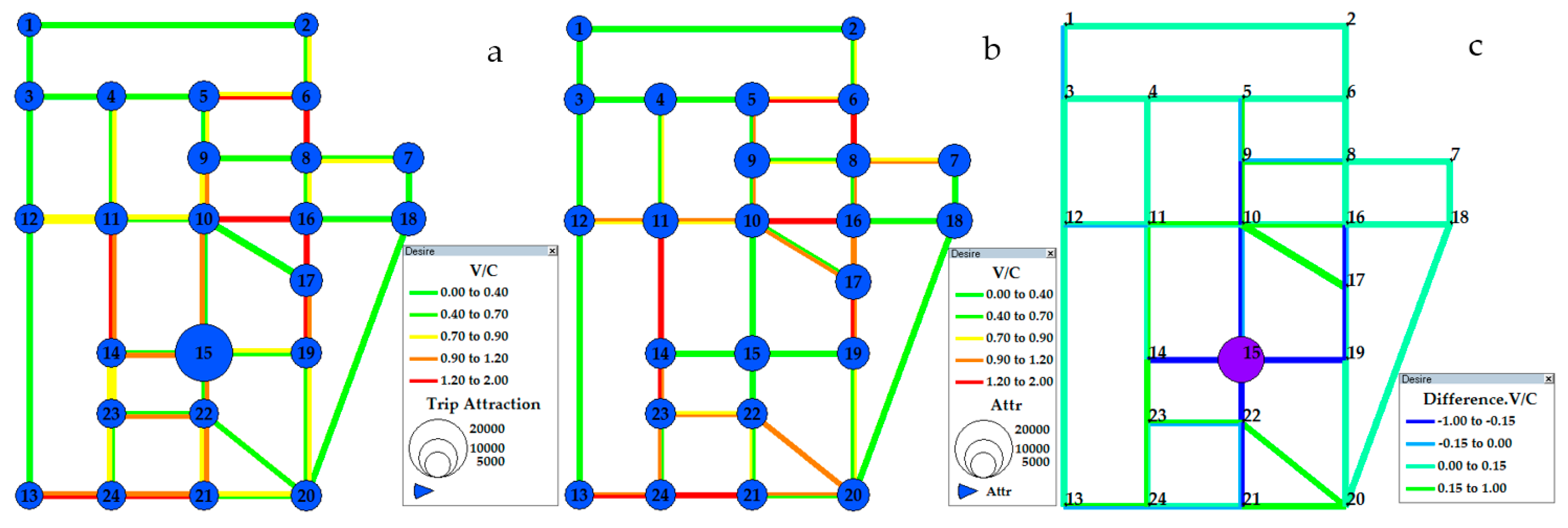
Experiment 2: This experiment is designed to analyze the impacts of multiple commercial centers on traveler’s behavior by the CDA model. The commercial centers can be categorized as static facilities in the CDA model. Hence, we adjust the constant term of the attraction measure at the destination zone to simulate the impacts of multiple centers. In this experiment, Zone 15 is assumed to be a central business district (CBD) and more attractive to travelers than the other zones. Here, we set the attraction measure at Zone 15 to be 15, and 1 for the other zones. Then, we adjust the attraction measure at Zone 8 to 15, assuming Zone 8 is a new commercial center. These two results are shown in Figure 8a,b, respectively. The color of links indicates the V/Cs of them, and the size of each traffic zone is proportional to its trip attraction. Obviously, Zone 8 will attract much more travelers after it becomes a commercial center by comparing Figure 8a,b. Furthermore, the differences of the network flow between these two results are shown in Figure 8c. Links are coded with darker colors if the negative differences in V/C are greater, which means that more travelers will pass through these links. The CDA model shows that with the increase of trip attraction at Zone 8, it will lead to an increase in the traffic volume on the links around the new commercial center and a decrease in the congestion level on the links around the other zones.
The influences of the static facilities on the network flow pattern and trip attraction in zones are discussed in the above experiments. The results are understandable and acceptable based on our experience. In the following, we mainly introduce the applications of the CDA model to two practical TDM strategies, the parking charge and congestion charge strategies. In simple words, the objective of the TDM is to make use of the existing transportation infrastructure in a more efficient way. TDM has been proved to be useful to ease traffic congestion in practice, which is helpful for building the sustainable transportation system and improving living quality.
Experiment 3: This experiment aims at showing the application of the CDA model for verifying the parking charge strategy. The strategy has been implemented in many cities around the world. It can not only balance the parking supply and demand but also have benefits for easing traffic congestion. In this experiment, we assume that the parking fee is related to the trip attraction of the corresponding zone and the functional relation between them is shown in Equation (21). Moreover, the parking fee is set to be high at those zones close to the commercial center. Only one commercial center, Zone 15, is involved. We adjust the coefficient a to 10 at Zone 15, 5 at the zones near Zone 15 (Zone 11, 10, 16, 17, 19, 22, 23, 14), and 1 at the other zones. The results without and with the strategy are shown in Figure 9a,b, respectively. Comparing Figure 9a,b, we can observe that less travelers will choose Zone 15 and the surrounding zones after implementing this strategy, which results from a relatively great increase in variable destination cost at these zones. This indicates that the charge level of each zone can be adjusted to control the attracted traffic volumes. It explains the benefits of the strategy in balancing the parking supply and demand. In addition, the differences in network flow between the two results are shown in Figure 9c. The links are coded with a darker color if the negative changes in V/C are greater. Obviously, the implementation of this strategy will lead to flow decreases on links around the zones with high charge level, which demonstrates its benefits in easing the congestion level.
Experiment 4: The CDA model is applied to reveal the effects of the congestion charge strategy on travelers’ behavior in this experiment. The congestion charge strategy and the parking charge strategy both can be regarded as the TDM strategies and affect the traveler’s behavior from an economic aspect, but there are differences between them. On the one hand, Glazer and Niskanen pointed out that the hourly parking price may induce demand because more parking spaces become available as travelers shorten their dwell times (some specific period in which travelers visit their destinations) [27]. Hence, the congestion charge strategy may perform better than the parking charge strategy for easing the traffic congestion level in certain situations. On the other hand, the congestion charge strategy is implemented only in the congested areas, and travelers must pay for their entrance or exit of the areas (which is obviously different from the parking charge strategy, because travelers will only be charged in their destinations for parking). Consequently, the CDA model cannot be adopted directly to handle this situation, because travelers should also be charged when they go across rather than end at the congested areas, which is not included in the model. Here, we exploit some network representation techniques to transform the original problem into the CDA problem. An example, used to illustrate the network modifications, is shown in Figure 10. The red circle represents the congested area. First, add several nodes between the congested area and each adjacent node (node EA, EB, EC, and ED). Then, add several links to connect any two nodes in the red circle (the dashed line in Figure 10). The cost on each dummy link is set to be the congestion fee, and the network outside the red circle is not modified. These modifications aim to make sure that travelers will pass through only one dummy link in the following three situations: (1) Zone E is the origin; (2) Zone E is the destination; (3) Zone E is the intermediate node, being neither the origin, nor the destination. Although there are many alternative paths to cross the congestion area between any two nodes in {EA, EB, EC, ED, E}, travelers will undoubtedly choose the shortest one containing only one dummy link. As a result, travelers will spend extra trip cost on the dummy links, which is equivalent to the congestion fee. Then, the problem is transformed into the CDA problem.
In this experiment, only one commercial center (Zone 15) is involved and the strategy is implemented only in Zone 15. The congestion fee is set to be 15, and the results without and with the strategy are shown in Figure 11a,b, respectively. Apparently, many travelers who choose Zone 15 as their destination originally change their trip destination after implementing the charge strategy, owing to the great increase in destination cost of Zone 15. Besides, there are greatly decreasing flows on the links directly connecting with Zone 15 and increasing flows on the links around but not connecting with Zone 15. It indicates that travelers avoid crossing Zone 15 and choose the alternative paths because of the congestion fee.
Experiment 3 and 4 introduce the applications of the CDA model to two practical TDM strategies. Our experiments demonstrate that the parking charge has effects on not only balancing the parking demand and supply but also easing the congestion level around the commercial center, and the congestion charge strategy may lead to the flow decreases on the links directly connecting with the congested area. These results show that the CDA model has good interpretations in the impacts of these strategies on travelers’ behavior in consideration of the spread of ITS. Consequently, the CDA model can provide reliable assessments of the TDM strategies, which is of great value in practice.

5. Conclusions

In modern urban transportation systems, it could be difficult for the traditional four-step travel demand forecasting model to achieve good performance in predicting the travel demand because of: (1) more alternative destinations (multiple commercial centers as the rapid development of the urban area); and (2) access to more accurate and detailed information with the help of ITS. These two factors mean that travelers may consider the destination and the travel path simultaneously, which differs from the assumption of the four-step model (travelers consider their destination and travel path in a sequential order). In this paper, the CDA model, in which the assumption is more closed to the travelers’ behavior, is adopted to handle this issue. The constant and variable terms in the attraction measure of destination are interpreted as the attraction of static facilities and congestion effect, respectively. Four experiments are conducted in the Sioux Falls network to examine: (1) differences in network flow pattern between the four-step and CDA model; (2) effects of multiple commercial centers on traveler’s behavior; (3) application of the CDA model to the parking charge strategy; and (4) application of the CDA model to the congestion charge strategy. Based on the experiment results, it can be concluded that it is of value to apply the CDA model on travel demand forecasting for modern urban transportations.
Besides, we present the MGP algorithm to solve the combined distribution and assignment problem in this paper. The MGP algorithm is developed on the basis of the GP algorithm, which has been proved a successful path-based algorithm to solve the TAP, and the MGP algorithm shifts path flows among all the active paths rather than from each non-shortest path to the shortest one. With the CDA model converted into a standard TAP by network representation method, the MGP algorithm can be easily adopted to solve the converted problem. Two road networks, Sioux Falls and Chicago Sketch, are used to conduct numerical experiments in order to demonstrate the new algorithm better than the widely used Evans’ two-stage method incorporated with the GP algorithm for solving the CDA model. Overall, the numerical results indicate that the new algorithm can search a solution with higher accuracy than the two-stage algorithm.

Author Contributions

Conceptualization, H.T. and M.D.; Methodology, H.T.; Validation, X.J. and Z.C.; Writing-Original Draft Preparation, H.T.; Writing-Review & Editing, X.J.; Supervision, M.D.; Funding Acquisition, M.D.

Funding

This research was funded by [Natural Science Foundation of China] grant number [71801079], [Fundamental Research Funds for the Central Universities] grant number [2017B12414], and [China Postdoctoral Science Foundation] grant number [2017M611680].

Conflicts of Interest

The authors declare no conflict of interest.

References

  1. Zhu, S.; Guo, K.; Guo, Y.; Tao, H.; Shi, Q. An adaptive signal control method with optimal detector locations. Sustainability 2019, 11, 727. [Google Scholar] [CrossRef]
  2. Ma, C.; Hao, W.; Wang, A.; Zhao, H. Developing a coordinated signal control system for urban ring road under the vehicle-infrastructure connected environment. IEEE Access 2018, 6, 52471–52478. [Google Scholar] [CrossRef]
  3. Wardrop, J.G. Some theoretical aspects of road traffic research. Proc. Inst. Civ. Eng. 1952, 1, 325–362. [Google Scholar] [CrossRef]
  4. Tomlin, J.A. Mathematical programming model for the combined distribution-assignment of traffic. Transp. Sci. 1971, 5, 122–140. [Google Scholar] [CrossRef]
  5. Florian, M.; Nguyen, S.; Ferland, J. On the combined distribution-assignment of traffic. Transp. Sci. 1971, 5, 120–140. [Google Scholar] [CrossRef]
  6. Evans, S. Derivation and analysis of some models for combining trip distribution and assignment. Transp. Res. 1976, 10, 37–57. [Google Scholar] [CrossRef]
  7. Oppenheim, N. Equilibrium trip distribution/assignment with variable destination cost. Transp. Res. Part B 1993, 27, 207–217. [Google Scholar] [CrossRef]
  8. Yao, J.; Chen, A.; Ryu, S.; Shi, F. A general unconstrained optimization formulation for the combined distribution and assignment problem. Transp. Res. Part B 2014, 59, 137–160. [Google Scholar] [CrossRef]
  9. Yang, H.; Bell, M.; Meng, Q. Modeling the capacity and level of service of urban transportation networks. Transp. Res. Part B 2000, 34, 255–275. [Google Scholar] [CrossRef]
  10. Cheng, L.; Du, M.; Rakha, H. Modeling and estimating the capacity of urban transportation network with rapid transit. Transport 2014, 29, 165–174. [Google Scholar] [CrossRef]
  11. Du, M.; Jiang, X.; Cheng, L. Alternative network robustness measure using system-wide transportation capacity for identifying critical links in road network. Adv. Mech. Eng. 2017, 9, 1–12. [Google Scholar] [CrossRef]
  12. Chen, A.; Yang, C.; Kongsomsaksakul, S.; Lee, M. Network-based accessibility measures for vulnerability analysis of degradable transportation networks. Netw. Spat. Econ. 2007, 7, 241–256. [Google Scholar] [CrossRef]
  13. Chen, A.; Kasikitwiwat, P. Modeling network capacity flexibility of transportation networks. Transp. Res. Part A 2011, 45, 105–117. [Google Scholar] [CrossRef]
  14. Chen, A.; Kasikitwiwat, P.; Yang, C. Alternate capacity reliability measures for transportation networks. J. Adv. Transp. 2013, 47, 79–104. [Google Scholar] [CrossRef]
  15. Yim, K.; Wong, S.C.; Chen, A.; Wong, C.K.; Lam, W.H.W. A reliability-based land use and transportation optimization model. Transp. Res. Part C 2011, 19, 351–362. [Google Scholar] [CrossRef]
  16. Gentile, G. Local user cost equilibrium: A bush-based algorithm for traffic assignment. Transp. Metr. A Transp. Sci. 2014, 10, 15–54. [Google Scholar] [CrossRef]
  17. Sheffi, Y. Urban Transportation Networks: Equilibrium Analysis with Mathematical Programming Methods; Prentice Hall: Englewood Cliffs, NJ, USA, 1985; pp. 164–180. [Google Scholar]
  18. Jayakrishnan, R.; Tsai, W.; Prashker, J.; Rajadhyaksha, S. A Faster Path-based Algorithm for Traffic Assignment. Transp. Res. Rec. 1994, 1443, 75–83. [Google Scholar]
  19. Bekhor, S.; Toledo, T. Investigating path-based solution algorithms to the stochastic user equilibrium problem. Transp. Res. Part B 2005, 39, 279–295. [Google Scholar] [CrossRef]
  20. Xu, X.; Chen, A.; Zhou, Z.; Bekhor, S. Path-based algorithms to solve c-logit stochastic user equilibrium assignment problem. Transp. Res. Rec. J. Transp. Board 2012, 2279, 21–30. [Google Scholar] [CrossRef]
  21. Chen, A.; Zhou, Z.; Xu, X. A self-adaptive gradient projection algorithm for the nonadditive traffic equilibrium problem. Comput. Oper. Res. 2012, 43, 68–77. [Google Scholar] [CrossRef]
  22. Ryu, S.; Chen, A.; Choi, K. A modified gradient projection algorithm for solving the elastic demand traffic assignment problem. Comput. Oper. Res. 2014, 47, 61–71. [Google Scholar] [CrossRef]
  23. Ryu, S.; Chen, A.; Choi, K. Solving the combined modal split and traffic assignment problem with two types of transit impedance function. Eur. J. Oper. Res. 2017, 257, 870–880. [Google Scholar] [CrossRef]
  24. Bureau of Public Roads. Traffic Assignment Manual; US Department of Commerce. Urban Planning Division: Washington, DC, USA, 1964.
  25. Boyce, D. Is the sequential travel forecasting procedure counterproductive? J. Urban Plan. Dev. 2002, 128, 169–183. [Google Scholar] [CrossRef]
  26. Xu, M.; Chen, A.; Gao, Z. An improved origin-based algorithm for solving the combined distribution and assignment problem. Eur. J. Oper. Res. 2008, 188, 354–369. [Google Scholar] [CrossRef]
  27. Glazer, A.; Niskanen, E. Parking fees and congestion. Reg. Sci. Urban Econ. 1992, 22, 123–132. [Google Scholar] [CrossRef] [Green Version]
Figure 1. Network representation for solving the CDA problem.
Sustainability 11 02167 g001
Figure 2. A simple network with three alternative equilibrium paths.
Sustainability 11 02167 g002
Figure 3. An augmented network to illustrate the path generation scheme.
Sustainability 11 02167 g003
Figure 4. Flowchart of the MGP algorithm for solving the converted CDA problem.
Sustainability 11 02167 g004
Figure 5. RGAP versus CPU time on Sioux Falls network.
Sustainability 11 02167 g005
Figure 6. RGAP versus CPU time on Chicago Sketch network.
Sustainability 11 02167 g006
Figure 7. Absolute differences in V/C on each link between the four-step model and the CDA model.
Sustainability 11 02167 g007
Figure 8. An example to illustrate the impacts of more commercial centers on traveler’s behavior: (a) the results of one commercial center, Zone 15; (b) the results of two commercial centers, Zone 8 and 15; (c) the differences in the network flow between the two results.
Sustainability 11 02167 g008
Figure 9. An example to illustrate the impacts of the parking charge strategy on traveler’s behavior: (a) without the parking charge strategy; (b) with the parking charge strategy; (c) the differences on the network flow between the two results.
Sustainability 11 02167 g009
Figure 10. Network modifications represent the congestion charge strategy in zone E: (a) the original network; (b) the modified network.
Sustainability 11 02167 g010
Figure 11. An example to illustrate the impacts of the congestion charge strategy on traveler’s behavior: (a) without the congestion charge strategy; (b) with the congestion charge strategy implemented in zone 15; (c) the differences in the network flow and the trip attraction between the two results.
Sustainability 11 02167 g011
Table 1. Comparative performance of the TSM-GP and NR-MGP algorithms on the test networks.
Test NetworkTimeTSM-GPNR-MGP
RGAPObj. FunctionRGAPObj. Function
Sioux Falls0.5 s2.2 × 10−313,248,368.427 × 10−413,179,746.80
1 s2.4 × 10−413,236,184.031 × 10−413,179,601.59
5 s4.5 × 10−513,234,443.851.1 × 10−1013,179,596.86
Chicago Sketch0.5 h3.1 × 10−329,809,430.393.6 × 10−329,794,571.50
1 h1.3 × 10−329,807,013.271.3 × 10−329,790,654.11
5 h1.8 × 10−329,806,811.809.3 × 10−529,789,583.94

