A Novel Hybrid Evolutionary Data-Intelligence Algorithm for Irrigation and Power Production Management: Application to Multi-Purpose Reservoir Systems

Abstract

Multi-purpose advanced systems are considered a complex problem in water resource management, and the use of data-intelligence methodologies in operating such systems provides major advantages for decision-makers. The current research is devoted to the implementation of hybrid novel meta-heuristic algorithms (e.g., the bat algorithm (BA) and particle swarm optimization (PSO) algorithm) to formulate multi-purpose systems for power production and irrigation supply. The proposed hybrid modelling method was applied for the multi-purpose reservoir system of Bhadra Dam, which is located in the state of Karnataka, India. The average monthly demand for irrigation is 142.14 (10⁶ m³), and the amount of released water based on the new hybrid algorithm (NHA) is 141.25 (10⁶ m³). Compared with the shark algorithm (SA), BA, weed algorithm (WA), PSO algorithm, and genetic algorithm (GA), the NHA decreased the computation time by 28%, 36%, 39%, 82%, and 88%, respectively, which represents an excellent enhancement result. The amount of released water based on the proposed hybrid method attains a more reliable index for the volumetric percentage and provides a more effective operation rule for supplying the irrigation demand. Additionally, the average demand for power production is 18.90 (10⁶ kwh), whereas the NHA produces 18.09 (10⁶ kwh) of power. Power production utilizing the NHA’s operation rule achieved a sufficient magnitude relative to that of stand-alone models, such as the BA, PSO, WA, SA, and GA. The excellent proficiency of the developed intelligence expert system is the result of the hybrid structure of the BA and PSO algorithm and the substitution of weaker solutions in each algorithm with better solutions from other algorithms. The main advantage of the proposed NHA is its ability to increase the diversity of solutions and hence avoid the worst possible solutions obtained using BA, that is, preventing a decrease in local optima. In addition, the NHA enhances the convergence rate obtained using the PSO algorithm. Hence, the proposed NHA as an intelligence model could contribute to providing reliable solutions for complex multi-purpose reservoir systems to optimize the operation rule for similar reservoir systems worldwide.

1. Introduction

Water resource management attempts to control water scarcity during successive drought periods [1]. Climate change phenomena and increasing population demands cause serious natural dilemmas that necessitate the operation of an optimal and reliable system for managing water resources [2,3,4]. The optimal operation of stored water resources in the form of reservoirs behind dams is an important and complicated issue for decision-makers and designers worldwide, because optimal operations can decrease the expenditure of constructing large dams for policymakers in the water resource management field [5]. Thus, several studies have investigated the optimal operation of reservoirs to satisfy downstream consumer demands and supply water based on high certainty [6,7,8]. Recently, mathematical models and evolutionary algorithms have been used in the management and planning of water resources [9,10,11,12]. The problem with optimal operations related to water reservoirs can be defined within the framework of an optimization problem [13,14,15]. Thus, meta-heuristic algorithms, which are powerful tools, are used for solving such problems [16]. The water supply problem includes several factors, such as environmental, municipal, and agricultural supply demands [10,17]. Consequently, solving these real-life problems can promote comprehensive visions and plans for the improved management of water resource applications. Various challenges are observed in solving the reservoir operation problem, including the stochasticity in the system input and the uncertainties in the computation of non-linear factors, such as water loss from the reservoir. In addition, the needs of the stakeholders influence the allocation of the reservoir water, and accommodating these needs in the operation of the reservoir is a complex task for decision-makers [18,19,20,21,22]. Furthermore, climate change is one of the most influential variables that might negatively affect the pattern of the water supply, and addressing these problems is critical for decision-makers. Therefore, defining an appropriate optimization algorithm with effective mathematical models is essential to providing effective operation guidance and informing comprehensive planning for current and future periods. The successful determination of optimal operation procedures for reservoir water systems could provide decision-makers with effective tools to optimize the allocation and distribution of these resources [23,24,25]. In fact, most mathematical models, such as nonlinear programming, cannot be accurately adapted with multi-objective problems and perform the optimization procedure in a reasonable time period. In addition, these models should be able to consider effective parameters that influence the optimization process, such as climate change conditions or uncertain inflow to reservoirs [10]. Furthermore, in a few cases, the proper identification of dam and reservoir water system features (complex problems) requires the application of optimization tools as well as water allocation tools, such as game theory methods, to effectively operate the system [23,24,25]. Therefore, optimization algorithms capable of receiving and handling large data (non-stationary and stochastic in nature) under different climate change conditions could be used as effective tools for planning and managing water resources. Notably, models that are not limited to one specific problem or one particular boundary condition might not suitable for dam and reservoir water systems, because reservoir operation problems usually present different boundary conditions and are influenced by climate change conditions [25]. The water released for irrigation demands is very important because the development of agriculture in a basin is dependent on the fair allocation to the downstream consumers [17]. Therefore, supplying enough water to meet irrigation water demands requires accurate planning to avoid the risk of serious irrigation deficiencies, which will negatively affect crop production. In addition, water released from the reservoir is dependent on the physical characteristics of the dam and reservoir system, and these characteristics can be highly non-linear, such as the interrelationship among the elevation, surface area, and storage in the reservoir [18]. In this context, generating optimal operation rules for water release based on nonlinear or linear objective functions with different constraints is considered an important problem for policymakers [20].

1.1. Background

Many research efforts have been developed to investigate the potential of using meta-heuristic algorithms to generate optimal operation rules for dams and reservoir water systems. The honey bee optimization algorithm (HBOA) with a mutation operator has been utilized to minimize hydropower deficits [25]. This algorithm has been applied in multiple reservoirs, such as the Karun and Dez reservoirs located in southern Iran. The minimum and maximum operational storage for Dez and Karun are set to (453 and 2813) and (1518 and 2802) MCM (million of cubic metres), respectively. The researchers performed a comprehensive sensitivity analysis and compared the results with those of the genetic algorithm (GA) to verify the outstanding performance of this method. The results indicated that the improved HBOA could be a global solution based on less iteration than that of the GA and the particle swarm optimization (PSO) algorithm.

Genetic programming (GP) is one of the most effective optimization algorithms and has been applied for several optimization problems in the hydrology field. GP was used as an optimization tool to optimize the operation rules of a reservoir to meet the irrigation demands [26], where the released water was considered a decision variable. The methodology was applied to the Karaj reservoir as a case study. This reservoir is located on the Karaj River and has an active volume of 176 × 10⁶ m³ and an annual average inflow of 415.23 × 10⁶ m³. The released water based on the GA could meet downstream demand patterns effectively, and the annual average irrigation deficits based on the GA were 12% and 22% less than those achieved using the PSO algorithm and GA, respectively.

The PSO algorithm is a heuristic search tool used by Ostadrahimi et al. [27] to extract rule curves for optimizing the hydropower generation of multi-reservoir operations. The case study used to examine the PSO algorithm was a relatively small section of the Columbia River basin, which includes the Mica, Libby, and Grand Coulee reservoirs. The released water was considered the decision variable, and reservoir storage was considered the state variable. The results indicated that hydropower generation could be increased by approximately 12% and 15% using the PSO algorithm compared with the HBOA and GA, respectively. Additionally, the convergence rate experienced using the PSO algorithm was relatively faster than that of GA and HBOA.

Nonlinear order rule curves have been used with GAs for the operation of water systems with the aim of decreasing irrigation deficiencies, and the results have shown that released water based on the third-order rule curve could supply downstream demands well [28]. Another study conducted reservoir operations of a three-reservoir system (Karoon4, Khersan1, and Karoon3) via GP [29]. The capacities of those reservoirs are 2190, 332.55, and 2522 × 10⁶ m³, respectively. The aim of these studies was to minimize irrigation deficiencies. Downstream demands were supplied based on a volumetric reliability index of approximately 90%, while the supply for the downstream irrigation demand based on the GA was accompanied by high deficiencies during the operation period of the reservoir. Another study focused on the Karoon4 reservoir and utilized the water cycle algorithm (WCA) to increase the benefit of hydropower generation based on the released water, and the results showed that compared with the PSO algorithm and the GA, the WCA increased the annual benefit of hydropower generation by approximately 30% and 40%, respectively [30]. For the same reservoir, Haddad et al. [31] tested the biography-based optimization (BBO) algorithm for increasing hydropower generation. The results showed the high ability of the BBO algorithm based on a fast convergence speed and highly accurate computations.

An adaptive PSO algorithm was considered in another study [32]. This algorithm was modified based on the correction of the inertia coefficient. Additionally, the new method was used for multi-reservoir operations in a large-scale basin. The proposed method was implemented in the Three Gorges Project, with 42.23 bkW hydropower generation, and the XiLuoDo Project (XLDP), with 30.10 bkW. The new method had faster convergence and could yield solutions that were close to the global solution [32].

For the Karoon4 reservoir, Haddad et al. [31] tested the BBO algorithm for increasing hydropower generation. The results showed the high ability of the BBO algorithm based on a fast convergence speed and highly accurate computations.

The imperialist competitive algorithm (ICA) optimized ten system reservoirs with the aim of increasing power generation. The results showed that the ICA could increase annual power generation and yield the best solution based on fewer iterations during the convergence process [33].

A comparative study has been carried out by Azizipour et al. [8] to optimize the performance of a multi-reservoir system based on the weed algorithm (WA), GA, and PSO algorithm with the aim of decreasing irrigation deficiencies. This study focused on single and multi-reservoir operations of Dez reservoir, which has an average annual inflow to the reservoir of approximately 5950 million cubic meter per year. The results showed that the method could decrease the vulnerability index by approximately 12%, which reduced the deficiency of the operation based on the applied algorithm.

Another comparative study by Ehteram et al. [34] utilized the shark algorithm (SA) to optimize the performance of a multi-reservoir system for increasing hydropower generation in China. The maximum capacity of the hydropower plant was 600 MW. This algorithm is based on the rotational movement of sharks for escaping local optima. The SA could increase the convergence speed compared with the GA and PSO algorithms, and the annual power production was increased by approximately 20% and 40% compared with that of the PSO algorithm and GA, respectively.

The krill algorithm (KA) based on the swarm behaviors of krill is an advanced method used to increase the benefits of hydropower generation for multi-reservoir operations of the Timah reservoir located in Perlis, Malaysia [35]. This reservoir has a storage capacity between 28.74 × 106 and 40 × 106 m³. The results indicated that compared with the PSO algorithm and the GA, the KA could increase the annual benefits of power generation by 12% and 15%, respectively. Additionally, the convergence velocity for the KA was considerable.

The spider monkey algorithm (SMA) has been applied to the Karun reservoir by Ehteram et al. [35] for increasing hydropower generation, where the algorithm is based on the personal and swarm efforts of monkeys to find the best position for acquiring food. The results indicated that the algorithm performed better than the bat algorithm (BA), PSO algorithm, and GA, because it seeks to realize global solutions and convergence velocities.

However, the previous algorithms have key problems. For example, the GA traps local optima for certain multi-reservoir systems or exhibits slow convergence for certain problems [35]. The PSO algorithm encounters immature solutions with early convergence, which is a problem for this algorithm [35]. The BA requires the accurate determination of random parameters, such as maximum frequency, loudness, and pulsation rate, and may also trap local optima for complex engineering problems [3]. Studies have attempted to solve the different weaknesses of the various algorithms. For example, one study used the hybrid gravitational search algorithm (GSA) with GA, where GSA was used to provide a basic solution domain of problems and then genetic operators within the GA were used for upgrading the solutions [36]. A novel PSO algorithm with mutation strategies was introduced to provide solutions, and was then updated by a time-varying acceleration PSO algorithm to achieve the optimal solutions [37]. A hybrid PSO–GA was used to improve the balance between exploration and exploitation ability of the PSO algorithm based on genetic operators [38]. A parameter-free penalty function for the BBO was used to solve reliability redundancy allocation problems [39]. An improved artificial bee colony (ABC) based on the foraging behavior of global and guided best honeybees was used to solve complex optimization tasks [40]. However, these different algorithms have different weaknesses that should be improved. Note that the motivation for exploring a more robust and stable meta-heuristic method for modelling reservoir operation systems is still an ongoing focus for research on water resources by expert system scholars.

1.2. Problem Statement and Novelty

The studied problem is highly complex, and the main motivation behind establishing the current research is to discover the optimal solution for multi-purpose hydropower systems. The complexity arises from the highly stochastic relationship between optimal reservoir releases and various hydrological elements (e.g., water storage, water loss, inflow amount, and actual water demand). The maximized hydropower production constraint is not the only predominant variable for the optimization function, however, irrigation demands and sustainable water storage are tremendously important variables that affect this function. Such conditions of the multi-reservoir water system make the generation of optimal operation rules using a particular optimization algorithm a great challenge for researchers and decision-makers. Therefore, relying on one optimization algorithm to solve such a complex optimization application may be insufficient even when using a highly advanced algorithm. The main concerns in multi-reservoir water systems in terms of optimization include the search for the global optima of the system domain and the time required for convergence. For example, the BA is a well-known meta-heuristic approach that functions as a suitable tool for solving optimization problems [41,42,43]. Bozorg-Haddad et al. [44] applied the BA for reservoir operations with the aim of increasing power generation, and although power production could be increased, the BA is accompanied by certain weaknesses. One of the main problems is trapped local optima, although the algorithm exhibited a relatively fast convergence rate [44]. Alternatively, the PSO algorithm is known as an effective optimization algorithm in terms of its searching ability to achieve the global optima [5,32,45]. The local and global versions of this algorithm provide direct solutions to attain the optimum solution, while its drawback is the slow convergence rate. Thus, the problems associated with the BA and PSO algorithm, that is, trapping in local optima and slow convergence, respectively, motivated the authors to conduct the current study.

In this study, a new method based on hybridizing two meta-heuristic model structures (BA and PSO algorithm), namely the new hybrid algorithm (NHA), is proposed and developed to generate optimal operation rules for a multi-purpose reservoir water system. Conceptually, the proposed NHA model intends to introduce a hybrid algorithm structure that can replace the weakness of each algorithm with other algorithms. The PSO algorithm is used based on a hybrid framework to improve the BA’s ability to search for the global optima, while the BA is used to speed up the convergence rate. In this fashion, the main innovation of this paper is the proposition of an optimization model that can generate optimal operation rules for multi-purpose water operating systems with a high ability to search for global optima with a relatively high convergence rate.

Therefore, the novelty of the current research is focused mainly on two points: (1) introducing a hybrid optimization algorithm that can expand the search domain with sufficient diversity to avoid trapping the local optima and (2) creating an algorithm that is flexible enough to handle multi-purpose systems. To this end, the proposed algorithm should be examined using different benchmark functions to ensure its ability to achieve the global optima. In addition, the algorithm should be applied to a multi-purpose reservoir with different demands, and its results should be examined against the required system’s purposes to achieve effective and reliable operations. Furthermore, the current research provides insights on several performance indexes proposed to evaluate the achieved results.

1.3. Research Objectives

The main objective of this study is to propose the NHA to generate optimal operation rules for a multi-purpose reservoir water system, which is of importance for water resource supply and management worldwide. Therefore, a multi-purpose reservoir water system in India, namely the Bhadra reservoir system, which both supplies irrigation demands and produces power, is used in this study to examine the proposed optimization algorithm. In addition, several optimization algorithms and the proposed hybrid algorithm were applied to examine the effectiveness of the proposed NHA over the other algorithms. On the basis of the operations, a comprehensive analysis of the ability of the NHA to achieve the global optima and the convergence rate was carried out.

2. Methodological Overview

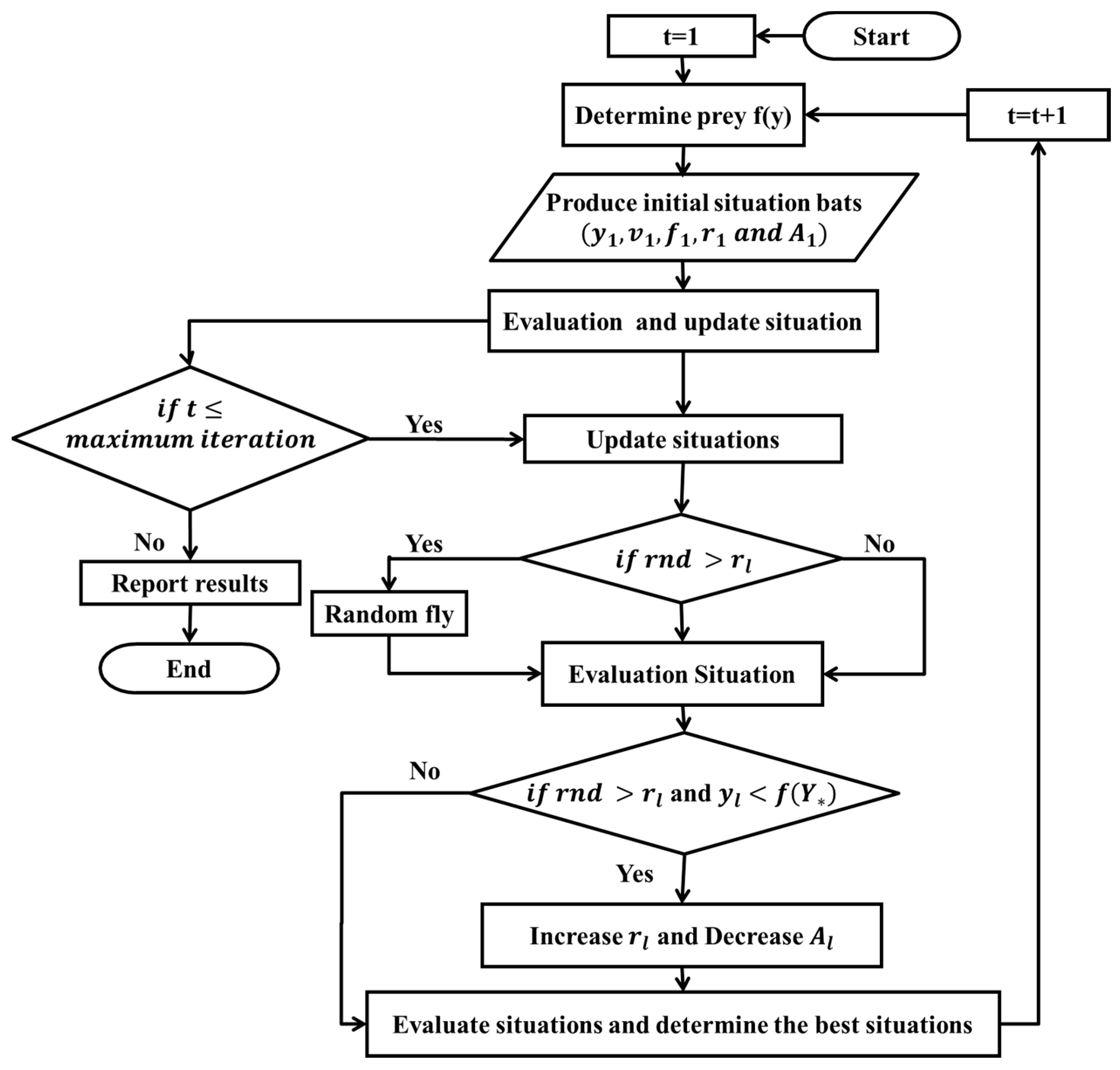
2.1. Bat Algorithm (BA)

Bats can produce sounds and receive the echo of the sounds from surrounding objects [41]. Thus, they can identify an obstacle from prey based on the received frequencies. The BA is based on the following assumptions:

• Echolocation is used by all bats, and this ability is helpful for identifying prey from obstacles.
• Bats fly at a random velocity, vl, and at a random location, xl. The frequency of a bat is fl. A0 and $\lambda$ represent the loudness and wavelength of bats, respectively.
• The loudness of bats varies from A0 (i.e., a large positive number) to Amin.

The velocity, location, and frequency are updated based on the following equations [46]:

$$f_l=f_{\min }+\left(f_{\max }-f_{\min }\right)\times \beta ,$$

(1)

$$v_l\left(t\right)=\left[y_l\left(t-1\right)-Y_{*}\right]\times f_l,$$

(2)

$$y_l\left(t\right)=y_l\left(t-1\right)+v_l\left(t\right)\times t,$$

(3)

where $f_l$ is the frequency; $f_{\min }$ is the minimum frequency; $f_{\max }$ is the maximum frequency; $\beta$ is the random value between 0 and 1; $Y_{*}$ is the best position of bats; $v_l\left(t\right)$ is the current velocity of bats; $y_l\left(t\right)$ is the current position of bats; and t is the time step.

A local search is considered based on the following formula using a random walk algorithm, and this level is referred to as the random fly level [41,42].

$$y\left(t\right)=y\left(t-1\right)+\epsilon A\left(t\right),$$

(4)

where $\epsilon$ is a random value between −1 and 1 and $A\left(t\right)$ is the loudness.

The loudness (A_t) and pulsation rate (r_l) are updated in each iteration of the algorithms. The value for loudness decreases and the pulsation rate increases when the bats find their prey. The pulsation rate for the generated sounds is updated based on the following equation [47]:

$$r_l^{t+1}=r_l^0\left[1-\exp \left(-\gamma t\right)\right]A_l^{t+1}=\alpha A_l^t,$$

(5)

where $r_l^{t+1}$ represents the new pulsation rate and $\alpha$ and $\gamma$ are constant values. Figure 1 shows the different levels for the BA.

2.2. Particle Swarm Optimization (PSO) Algorithm

If the search space is considered in the D dimension, the position of the particles is shown by $X_i={\left(x_{i1},x_{i2},\dots ,x_{iD}\right)}^T$, whereas the velocity is represented by $V_i={\left(v_{i1},v_{i2},\dots ,v_{iD}\right)}^T$. $P_i={\left(p_{i1},p_{i2},\dots ,p_{id}\right)}^T$ is considered the best prior calculated position, and the index g in the equations is used to determine the best particle among other particles based on the quality of the objective function. The position and velocity for the PSO algorithm are updated based on the following equations [48]:

$$v_{id}^{n+1}=\chi \left[w{v}_{id}^n+c_1{r}_1^n\frac{\left(p_{id}-x^n{}_{id}\right)}{\Delta t}+c_2{r}_2^n\frac{\left(p_{gd}-x_{id}^n\right)}{\Delta t}\right],$$

(6)

$$x_{id}^{n+1}=x_{id}^n+\Delta t{v}_{id}^{n+1},$$

(7)

where $v_{id}^{n+1}$ is the new velocity for the particles; $\chi$ is the constriction coefficient; $w$ is the inertia coefficient; $c_1$ and $c_2$ are the acceleration coefficients; $\Delta t$ is the time step; n is the time index; and $x_{id}^{n+1}$ is the new position of the particles.

First, the random parameters, as well as the initial velocity and position, are considered for the PSO algorithm [49]. The objective function is calculated for each member, and the best particle among the remaining particles is determined; then, the velocity and position are updated based on Equations (6) and (7), respectively [46,49]. Thus, the convergence criteria are stopped, and if the algorithm is satisfied, the algorithm finishes; otherwise, the algorithm returns to the first step. It should be noted here that the used version of the PSO in the current study is the modified one over the standard version. In this version, the one used, the weights are computed based on the following dynamical form equation:

$$\begin{array}{l}w=w_{end}+\left(w_{start}-w_{end}\right)\left(1-\frac{T}{G_{\max }}\right)\leftarrow if\left(p_{gd}\ne x_{id}\right)\\ w=w_{end}\leftarrow if\left(p_{gd}\right)=x_{id}\end{array}$$

(8)

where T is the number of iterations, $T\in \left[0,G_{\max }\right)$; pgd is the global bets position; wstart is the initial weight; and $w_{end}$ is the final value for the weight in the maximum iteration. Thus, the used PSO is an improved PSO that outperforms other versions.

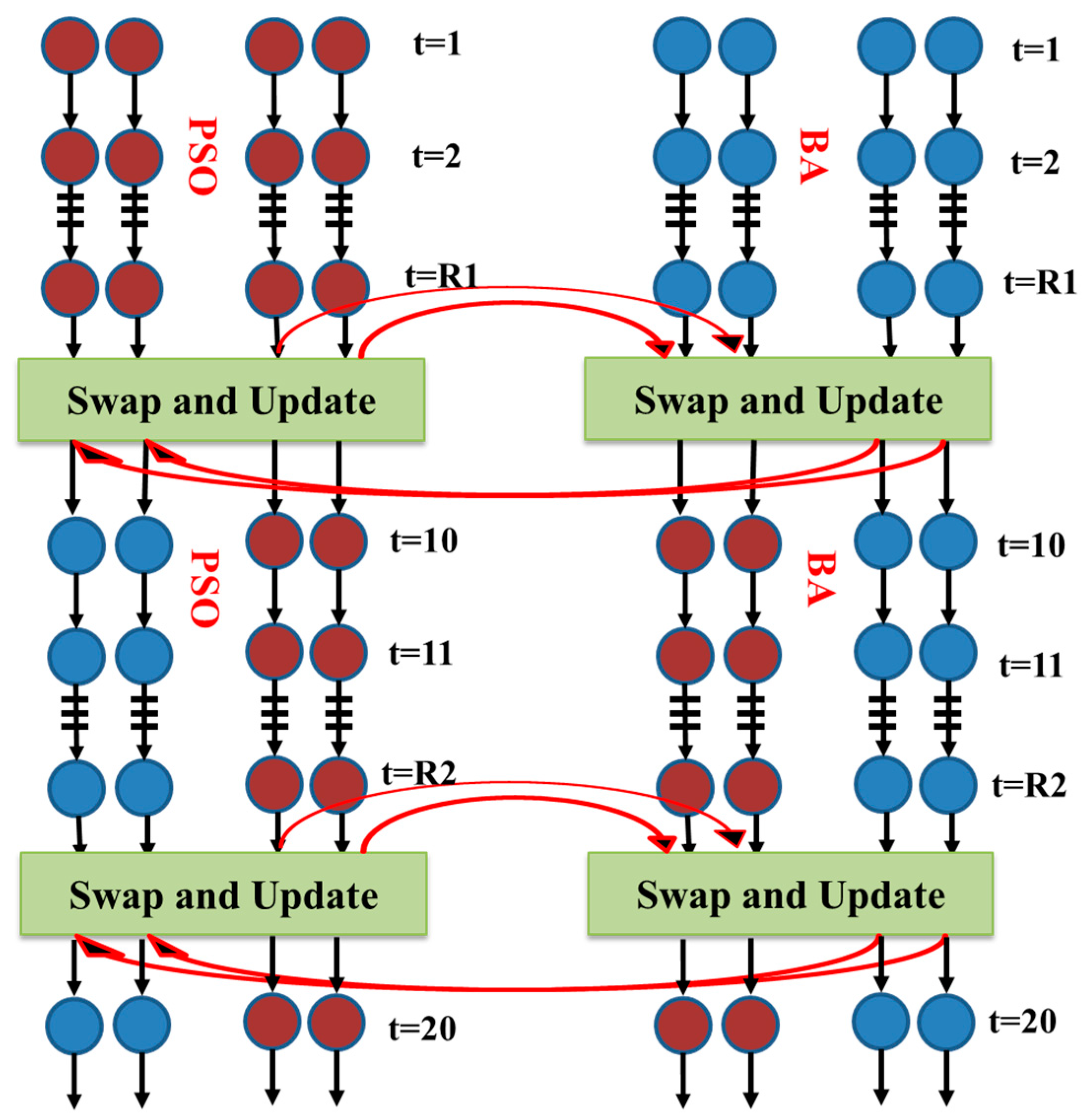
2.3. New Hybrid Algorithm (NHA)

The NHA is considered based on a parallel structure. Each algorithm acts based on an independent process, and then the output population of each algorithm is divided into subgroups (see Figure 2). Subsequently, a communication strategy shares information between the PSO algorithm and BA. The K agent of each algorithm, as the best member, is copied into the other algorithm instead of the worst solutions of the other algorithm. Thus, the worst solution achieved based on the BA is replaced using the one attained using the PSO algorithm. The total size population for the NHA is N, and N/2 represents the size population for the BA and PSO algorithm. R in Figure 2 represents the number of communication steps between the PSO algorithm and the BA, t denotes the current iteration count, and they are at the same level because two algorithms act simultaneously. Both the BA and PSO algorithms are executed concurrently within the same time step, and the achieved solutions at each time step are swapped between them synchronously. Accordingly, the NHA starts from an initial population as decision variables and ends when the convergence criteria are satisfied.

The NHA is based on the following levels:

• The random parameters are initialized for two algorithms, and then the velocity and position vectors are considered for the BA and PSO algorithms;
• The objective function is individually calculated for the two algorithms, and then the best member is determined for the two algorithms;
• The velocity and position are updated for the BA based on Equations (1)–(3), and the velocity and position are updated based on Equations (6) and (7), respectively;
• The K agent, as the best member of each algorithm, is copied to the other algorithms, which are substituted with the worst solutions of the other algorithm;
• The convergence criteria are checked, and if the algorithm is satisfied, the algorithm finishes; otherwise, the algorithm returns to the second step.

Although the proposed NHA procedure is established with a strong linkage between the BA and PSO algorithm, the NHA still faces a challenge during initialization for several random parameters for both algorithms. In addition, there is a need to adapt the random parameters for both the BA and the PSO algorithm within the definition of the NHA communication to enable it to simultaneously update within the mathematical model of the reservoir. This step adds more complexity within the proposed NHA for generating the operation rule to extract the optimal decision variables accurately for both algorithms.

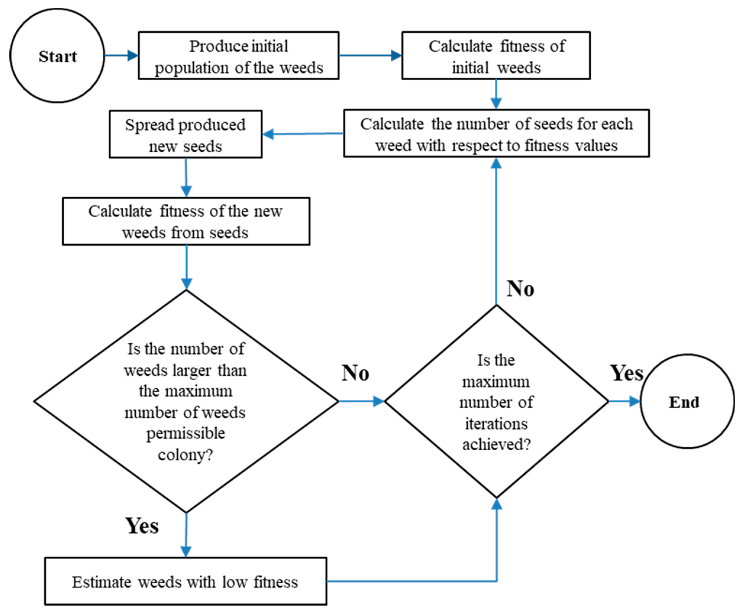
2.4. Weed Algorithm (WA)

The WA is based on the characteristics of weeds [50]. Weeds can grow spontaneously and adapt to their surroundings easily. The following assumptions are considered for the WA [34]:

• Weeds are grown based on seeds, which are spread throughout the environment.
• Weeds that grow close to each other are known as a colony, and they can produce seeds based on their equality.
• Each produced seed distributes randomly throughout the environment.
• The algorithm finishes when the number of weeds reaches the maximum number.
• The different levels for the WA are based on the following levels:
• First, the initial population of the algorithm (Pinitial) is considered, and the position of each weed in the environment (i.e., search space) is considered a decision variable.
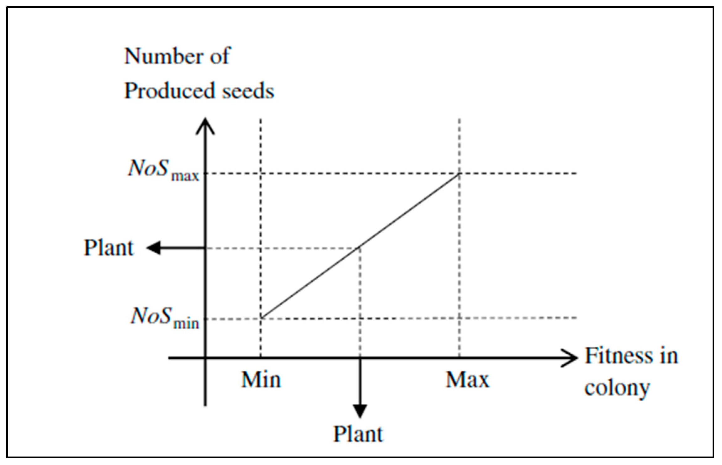
• The next level is known as the reproduction level. Reproduction causes new seeds to be produced from colonies, and the maximum and minimum numbers of seeds are $\left(N_0{S}_{\max }\right)$ and $\left(N_0{S}_{\min }\right)$, respectively (see Figure 3). Reproduction is an important level for the WA because there are two group solutions in the evolutionary algorithms. Appropriate solutions have a high chance of reproduction to continue the production of the best member for the next generation, and inappropriate solutions may have a weak chance of reproduction; however, they may have important information for the next levels of the algorithm. Thus, reproduction may be extended to inappropriate solutions that are not removed from the population, and they can continue their life based on suitable reproduction and the improvement in their quality. Some inappropriate solutions have important information, and this information can be used for the next levels of the algorithm.
• The produced seeds are distributed in the search space based on a normal distribution and zero mean.

The standard deviation for the distribution of seeds is variable and calculated based on the following equation [34,50]:

$${\sigma }_{iter}=\frac{\left(ite{r}_{\max }-iter\right)}{{\left(ite{r}_{\max }\right)}^n}\left({\sigma }_{initial}-{\sigma }_{final}\right),$$

(9)

where ${\sigma }_{iter}$ is the standard deviation; $ite{r}_{\max }$ is the maximum iteration number; $iter$ is the current iteration number; ${\sigma }_{initial}$ is the initial standard deviation; n is the nonlinear modulus; and ${\sigma }_{final}$ is the final standard deviation. Equation (9) shows that the distribution of the population is based on the standard deviation.

If weeds cannot produce seeds, they become extinct. Additionally, a number of seeds can be produced based on weeds limited to P_max, and there is competition among weeds because weeds of poor quality should be removed for population balance. Figure 4 shows the WA procedure.

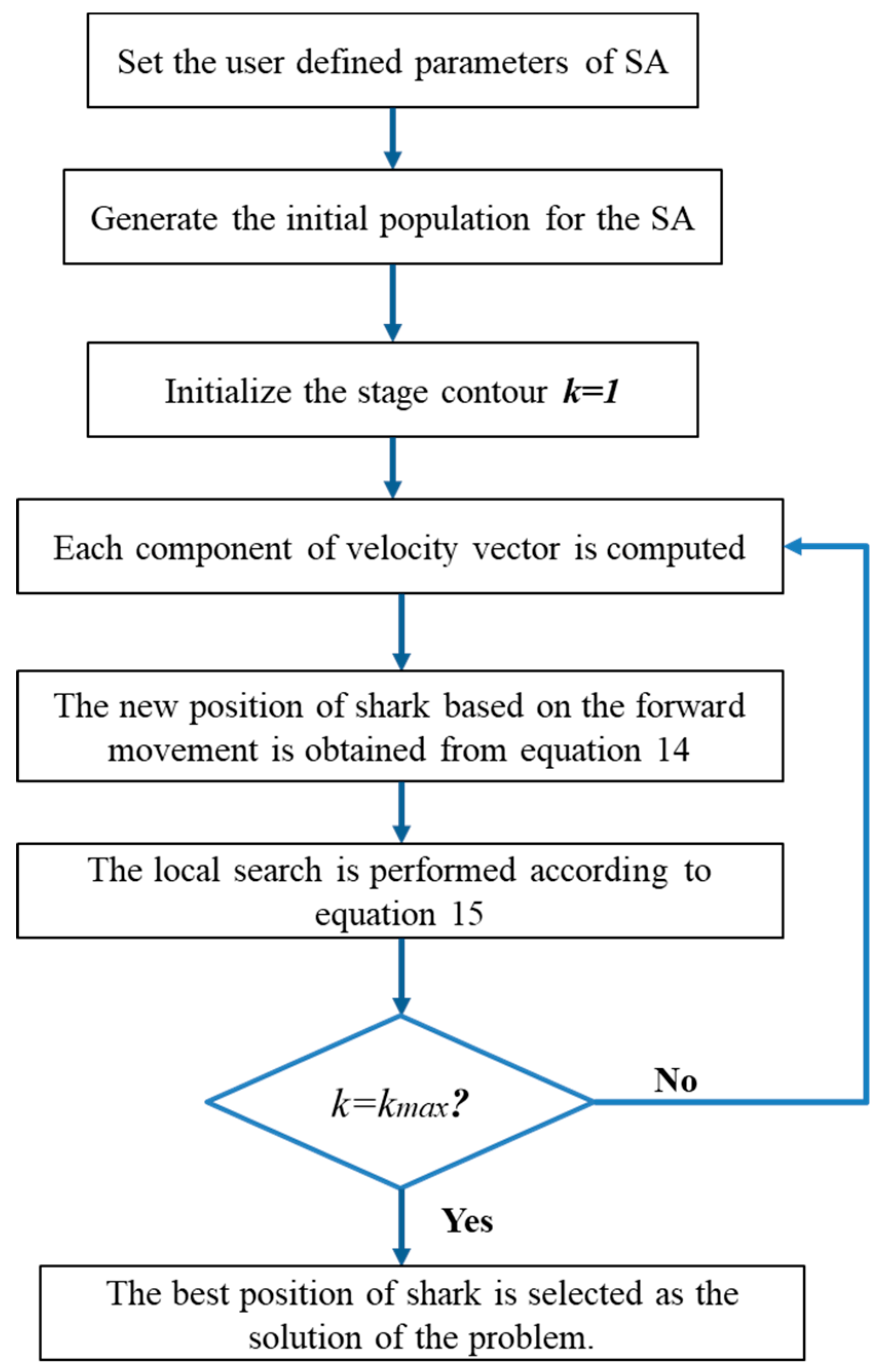
2.5. Shark Algorithm (SA)

Sharks have powerful olfactory receptors and can find their prey based on these receptors [51]. This algorithm acts based on the following assumptions [35]:

• Injured fish are considered to be prey for sharks, as fish bodies distribute blood throughout the sea. Additionally, injured fish have negligible speeds compared with sharks.
• The blood is distributed into the sea regularly, and the effect of water flow is not considered for blood distribution.
• Each injured fish is considered as one blood production resource for sharks; therefore, the olfactory receptors help sharks find their prey.
• The initial population for sharks is shown by $\left[X_1^1,X_2^1,\dots ,X_{NP}^1\right],NP=population\left(size\right)$. Each solution candidate or shark position can have the following components based on the following equation:

  $$X_i^1=\left[x_{i,1}^1,x_{i,2}^1,\dots x_{i,ND}^1\right],$$

  (10)

  where $X_i^1$ is the initial position vector; x¹_ij is the jth dimension of the shark position; and ND is the number of decision variables. The initial velocity for sharks is shown by $V_i^1=\left[v_{i,1}^1,v_{i,2}^1,\dots ,v_{i,ND}^1\right]$. The velocity components are considered based on the following equation:

  $$V_i^1=\left[v_{i,1}^1,v_{i,2}^1,\dots ,v_{i,ND}^1\right],i=1,\dots NP,$$

  (11)

  where $V_i^1$ is the initial velocity vector and v¹_ij is the jth dimension of the shark velocity. When the shark receives greater odour intensity, it moves faster towards its prey. Thus, if the odour intensity is considered an objective function, the velocity changes with the variation in the objective function based on the following equation:

  $$V_i^k={\eta }_k.R_1.\nabla \left(OF\right){|}_{x_i^k},$$

  (12)

  where ${\eta }_k$ is the number between 0 and 1; $R_1$ is the random number; and $OF$ is the objective function.

There is inertia in the shark’s movement, which should be considered in the shark velocity; thus, Equation (12) is modified based on the following equation:

$$v_{i,j}^k={\eta }_k.R_1.\frac{\partial \left(OF\right)}{\partial x_j}+\alpha .R_2.v_{i,j}^{k-1},$$

(13)

where $\alpha$ is the inertia coefficient and $R_2$ is the random value between 0 and 1.

Sharks have a specific domain for velocity. Their maximum velocity is 80 km/hr, and their minimum velocity is 20 km/hr. Thus, a velocity limit is considered, and Equation (13) is modified based on the following equation:

$$\left|v_{i,j}^k\right|=\min \left[{\left|{\eta }_k.R_1.\frac{\partial \left(OF\right)}{\partial x_j}\right|}_{x_{i,j}^k}+{\alpha }_k.R_2.v_{i,j}^{k-1}|,\left|{\beta }_k.v_{i,j}^{k-1}\right|\right],$$

(14)

where ${\beta }_k$ is the velocity limiter. Then, the shark position is updated based on the following equation:

$$Y_i^{k+1}=X_i^k+V_i^k\Delta t_k,$$

(15)

where $\Delta t_k$ is the time step and $Y_i^{k+1}$ is the new position for the shark. Sharks have a rotational movement operator. This operator indicates which shark can escape from the local optima, and the shark position based on the rotational movement is modified based on the following equation:

$$Z_i^{k+1,m}=Y_i^{k+1}+R_3.Y_i^{k+1},m=1,\dots ,M,$$

(16)

where $Z_i^{k+1,m}$ is the new shark position and M is the number of local searches for the sharks. Figure 5 shows the SA process.

2.6. Genetic Algorithm (GA)

First, the initial population for the GA consists of chromosomes, and the next population for the next generation is produced based on a repetitive process. The members with the best quality are selected, and the crossover operators and mutation operators are applied to the population to improve the solutions. The crossover is considered based on the following equation [35]:

$$Po{p}_i^{new}=\alpha Po{p}_i^{old}+\left(1-\alpha \right)Po{p}_j^{old},$$

(17)

$$Po{p}_j^{new}=\alpha Po{p}_j^{old}+\left(1-\alpha \right)Po{p}_i^{old},$$

(18)

where $Po{p}_i^{new}$ is the i-th child; $Po{p}_i^{old}$ is the i-th parent; $Po{p}_j^{old}$ is the j-th parent; $\alpha$ is the random number; and $Po{p}_j^{new}$ is the j-th child. The mutation is considered based on the following equation:

$$Po{p}_{j,i}^{new}=Va{r}_{j,i}^{law}+\beta \left(Va{r}_{j,i}^{h_i}-Va{r}_{j,i}^{law}\right),$$

(19)

where $Po{p}_{j,i}^{new}$ is the i-th new gene in the j-th chromosome; $Va{r}_{j,i}^{law}$ is the lower limit of the i-th gene in the j-th chromosome; $Va{r}_{j,i}^{h_i}$ is the upper limit of the i-th gene in the j-th chromosome; and $\beta$ is the random number. This crossover causes a change in the genes between two selected members when producing a new member. The mutation operator changes the chromosomes when producing new members.

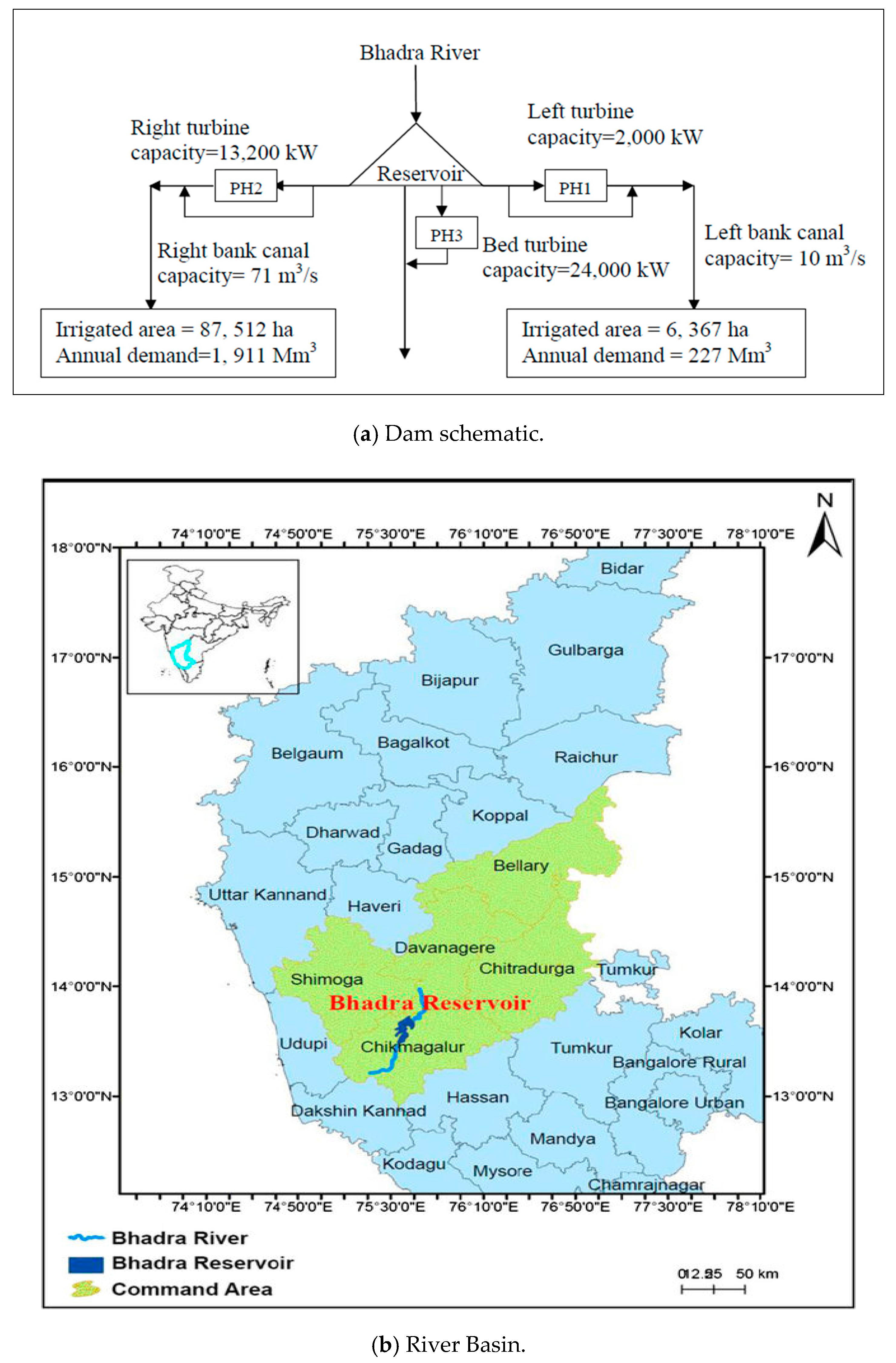
3. Case Study and Modelling Procedure

3.1. Benchmark Function

To test the superiority of the NHA, five global optimization problems were selected to compare the new method with the other methods (

Table 1. Details of benchmark functions.

Test Problem	Objective Function	Search Range	Optimum Value	Dimension	Characteristic	Acceptable Error (AE)
Schwefel function [52]	$f_1\left(x\right)={{\displaystyle \sum _{i=1}^D\left({\displaystyle \sum _{j=1}^i{x}_j}\right)}}^2$	[−100, 100]	0	30	Unimodal	1.0 × 10−3
Rastrigin [52]	$f_2\left(x\right)=10D+{\displaystyle \sum _{i=1}^D\left|x_i^2-10\cos \left(2\pi x_i\right)\right|}$	[−5.12, 5.12]	0	30	Multimodal	5.0 × 10−1
Dekkers and Aarts [52]	$f_3\left(x\right)={10}^5{x}_1^2+x_2^2-\left(x_1^2+x_2^2\right)+{10}^{-5}{\left(x_1^2+x_2^2\right)}^4$	[−20,20]	−24,777	2	Unimodal	1.0 × 10−5
Step function [52]	$f_4\left(x\right)={{\displaystyle \sum _{i=1}^D\left(\left|x_i+0.5\right|\right)}}^2$	[−100, 100]	0	30	Unimodal	1.0 × 10−3
Axis parallel function [52]	$f_5\left(x\right)={\displaystyle \sum _{i=1}^{D}i{x}_I^2}$	[−5.12, 5.12]	0	30	Unimodal	1.0 × 10−5

). A unimodal function has a single extremum, and multi-modal functions have multiple extrema; thus, if the exploration ability of the algorithm is weak, it cannot search the entire problem space.

3.2. Multi-Purpose Reservoir Operation

A multi-purpose reservoir system named Bhadra was considered to evaluate the NHA. The Bhadra Dam is located at 13°42′ N and 75°38′20″ E in the state of Karnataka. The location is characterized by a mean precipitation value of approximately 2320 mm, and 90% of the precipitation occurs during the monsoon period. Bhadra is a multi-purpose system reservoir that supplies water for demand and power production [53]. The active storage capacity for this reservoir is 1784 Mm³. The irrigation area is 6367 ha, and the total area of the left and right bank canals is 87,512 ha. Figure 6a shows the schematization of the dam and reservoir’s basin, and Figure 6b shows the geographical location of the catchment area of the basin. The features of the reservoir can be seen in

Table 2. Salient features of the Bhadra system.

Description	Quantity
Gross storage capacity	2025 Mm3
Live storage capacity	1784 Mm3
Dead storage capacity	241 Mm3
Average annual inflow	2845 Mm3
Left bank canal capacity	10 m3/s
Right bank canal capacity	71 m3/s
Left bank turbine capacity	2000 kW
Right bank turbine capacity (Phase2)	13,200 kW
Riverbed turbine capacity (Phase3)	24,000 kW

. Figure 6a shows the details for the system and Figure 6b shows the location of system on the river section. The command area for the river basin is 162,818 ha.

There are three turbines in this basin. The turbines are located along the right bank canal, left bank canal, and riverbed. The operating head for the right bank canal (Phase1) varies from 38.564 to 54.41 m, that of the left bank canal (Phase2) varies from 36.88 m to 56.69 m, and that of the riverbed varies from 36.88 to 55.12 m. When the water height is within the domain of the defined operation head, it moves in the direction of the turbines; otherwise, it is used for irrigation demands. Figure 7 shows the schematic of the multi-purpose system.

The necessary data, such as the monthly inflow, were obtained from the Water Resource Development Organization (Bangalore) and cover 10 years from 1990–1991 to 2000–2001. Semi-dry, garden, and paddy crops are important for this basin. The irrigation demand and power production should be supplied for the downstream region. Thus, the first objective function is to minimize irrigation deficiencies, and the second objective function is related to maximizing power production. Equation (20) is used for minimizing irrigation deficiencies:

$$SQDV={{\displaystyle \sum _{t=1}^{12}\left(D_{l,t}-R_{l,t}\right)}}^2+{{\displaystyle \sum _{t=1}^{12}\left(D_{r,t}-R_{r,t}\right)}}^2,$$

(20)

where $SQDV$ is the square deviation in the demand and released water; $D_{l,t}$ is the demand for the left bank canal; $D_{r,t}$ is the demand for the right bank canal; $R_{l,t}$ is the released water for the right bank canal; and $R_{r,t}$ is the released water for the left bank canal.

The second objective function is defined based on the following equation:

$$E={\displaystyle \sum _{t=1}^{12}\left(k_1{R}_{l,t}{H}_{l,t}+k_2{R}_{r,t}{H}_{r,t}+k_3{R}_{b,t}{H}_{b,t}\right)},$$

(21)

where $E$ is the produced energy; $k_1$, $k_2$, and $k_3$ represent the power coefficients; r is the right side of the bank canal, $R_{l,t}$, $R_{r,t}$, and $R_{b,t}$ represent the released water for the left and right bank canals and the river bed, respectively; and $H_{l,t}$, $H_{r,t}$, and $H_{b,t}$ represent the net head for the left and right canals and the riverbed, respectively. The head values are extracted based on a regression continuity Equation (21) based on storage values. The released water volume is a decision variable to be applied annually for ten years during the period between 1991 and 2000.

The continuity equation is defined based on the following equation:

$$S_{t+1}=S_t+I_t-\left(R_{lt}+R_{rt}+R_{bt}+E{V}_t+OV{F}_t\right),$$

(22)

where $S_{t+1}$ is the storage at time t + 1; $I_t$ is the inflow at time t; $E{V}_t$ is the evaporation loss; and $OV{F}_t$ is the overflow.

The constraints are considered based on the following equations:

• The storage constraint is as follows:

  $$S_{\min }\le S_t\le S_{\max },$$

  (23)

  where $S_{\max }$ is the maximum storage and $S_{\min }$ is the minimum storage.
• The power production constraints are as follows:

  $$k_1{R}_{l,t}{H}_{l,t}\le E_{1,\max },$$

  (24)

  $$k_2{R}_{r,t}{H}_{r,t}\le E_{2,\max },$$

  (25)

  $$k_3{R}_{bt}{H}_{bt}\le E_{3,\max },$$

  (26)

  where $E_{1,\max }$, $E_{2,\max }$, and $E_{3,\max }$ represent the maximum energy for the left canal, right canal, and riverbed, respectively.
• The canal capacity constraints are as follows:

  $$R_{l,t}\le C_{l,\max },$$

  (27)

  $$R_{r,t}\le C_{r,\max },$$

  (28)

  where $C_{l,\max }$ is the maximum capacity for the left canal and $C_{r,\max }$ is the maximum capacity for the right canal.
• The irrigation demands are as follows:

  $$D_{l,t}^{\min }\le R_{l,t}\le D_{l,r}^{\max },$$

  (29)

  $$D_{r,t}^{\min }\le R_{r,t}\le D_{r,t}^{\max },$$

  (30)

  where $D_{l,t}^{\min }$ is the minimum demand for the left canal; $D_{l,r}^{\max }$ is the maximum demand for the left canal; $D_{r,t}^{\min }$ is the minimum demand for the right canal; and $D_{r,t}^{\max }$ is the maximum demand for the right canal.
• The steady storage constraint is as follows:

  $$S_{13}=S_1.$$

  (31)

This constraint has been considered to guarantee no change in reservoir storage at the beginning of each cycle of operation in order to avoid the obstacle of reservoir carryover storage.

The above constraint causes the state condition to occur because the storage condition at the end of the year must be equivalent to that at the beginning of the year. There are two objective functions with opposite conditions; one objective function should be maximized, and the other objective function should be minimized. Thus, a weighted method is used to handle these two factors. There are two weight coefficients in Equation (32), and the irrigation demand has greater priority in this case study. When the irrigation demands are supplied, water is used for power production. Thus, Kumar and Reddy [53] suggested values of $w{t}_1=100$ and $w{t}_2=-1$ because the irrigation demands have greater importance for policymakers in this basin. The weighted aggregate sum product assessment is used to estimate and obtain accurate values for the weights [53]. Different weights are considered for different terms within the objective function, and their relative indexes are calculated to determine the best values for weights using NHA. Afterward, a ranking process is carried out utilizing the associated indexes for all the allocated weights. Finally, the multi-criteria decision process is used to identify the best allocated weight combination based on the highest rank.

The suggested values for these coefficients were calculated based on a sensitivity analysis by considering the variation in the objective function versus the variation in the value of the weight coefficients. Thus, the following equation is suggested for reservoir operations, and the aim of the problem is to minimize the following objective function:

$$F=w{t}_1{\displaystyle \sum _{t=1}^{12}\left[{\left(\frac{D_{l,t}-R_{l,t}}{D_{l,t}}\right)}^2+\left(\frac{D_{r,t}-R_{r,t}}{D_{r,t}}\right)\right]}+w{t}_2{\displaystyle \sum _{t=1}^{12}\left[\frac{E_{1,\max }-k_1{R}_{l,t}{H}_{l,t}}{E_{1,\max }}+\frac{E_{2,\max }-k_2{R}_{r,t}{H}_{r,t}}{E_{2,\max }}+\frac{E_{3,\max }-k_2{R}_{b,t}{H}_{b,t}}{E_{3,\max }}\right]},$$

(32)

where $w{t}_1$ and $w{t}_2$ represent the weight values; $E_{1,\max }$, $E_{2,\max }$, and $E_{3,\max }$ represent the maximum energy for the left canal, right canal, and riverbed, respectively; $k_1$, $k_2$, and $k_3$ represent the power coefficients; $R_{l,t}$, $R_{r,t}$, and $R_{b,t}$ represent the released water for the left and right bank canals and the riverbed, respectively; $H_{l,t}$, $H_{r,t}$, and $H_{b,t}$ represent the net head for the left and right canals and the riverbed, respectively; $D_{l,t}$ is the demand for the left bank canal; $D_{r,t}$ is the demand for the right bank canal; $R_{l,t}$ is the released water for the right bank canal; and $R_{r,t}$ is the released water for the left bank canal.

The decision variable for this problem is released water, the total number of decision variables is 36 for one year (number of time periods = 12), and the number of variables for released water each month is three (left canal, right canal, and riverbed). Thus, there are 360 decision variables in ten years. The hybrid algorithm is considered based on the following levels for reservoir operation:

• The decision variables for the left canal, right canal, and riverbed are initialized based on the initial matrix for the NHA. In fact, the released water for the downstream demands is considered as the initial population.
• The storage reservoir can be calculated based on the continuity equation, and the different constraints should be checked.
• If the constraints are not satisfied, the penalty functions are considered as violations; then, the objective function is calculated based on Equation (31).
• Then, the NHA process is considered for the optimization process based on the independent performances of the BA and PSO algorithm in the NHA.
• The convergence criteria are checked, and if the algorithm is satisfied, it finishes; otherwise, the algorithm returns to the second step.

In fact, the released water for the multi-reservoir system is considered a decision variable, which is inserted into the algorithms based on the initial matrix and population. Then, the reservoir storage should be calculated based on the inflow into the reservoir and the initial values of the decision variables. Subsequently, the storage and released water should be compared with the permissible value so that they are not more or less than the permissible value. Then, the objective function for each member or decision variable is calculated for the total operational period. Then, the operators of the different algorithms are applied to the population and decision variables, and the algorithms continue until the convergence criterion is satisfied.

4. Modelling Evaluation Indexes

It is necessary to evaluate the utilized evolutionary algorithms to investigate their performance for downstream irritation supply. Thus, three important indexes are defined based on the following information.

• Volumetric reliability index. This index is based on the ratio of released water to irrigation demands. Thus, a high percentage of this index represents the high performance of each algorithm.

  $${\alpha }_V=1-\frac{N_{t=1}^T\left(D_t>R_t\right)}{T},$$

  (33)

  where ${\alpha }_V$ is the volumetric reliability; $R_t$ is the released water; $D_t$ is the demand; $N_{t=1}^T\left(D_t>R_t\right)$ is the number of periods in which demand is not supplied; and T is the total number of operational periods.
• Vulnerability index. This index represents the maximum intensity of the failure that occurred during the operation period of a system. The periods for which irritation demands are not met are known as failure periods or critical periods, and maximum deficiency occurrences during these periods are represented by the vulnerability index; thus, a low percentage for this index is preferable [35].

  $$\lambda =Ma{x}_{t=1}^T\left(\frac{D_t-R_t}{D_t}\right)\times 100.$$

  (34)
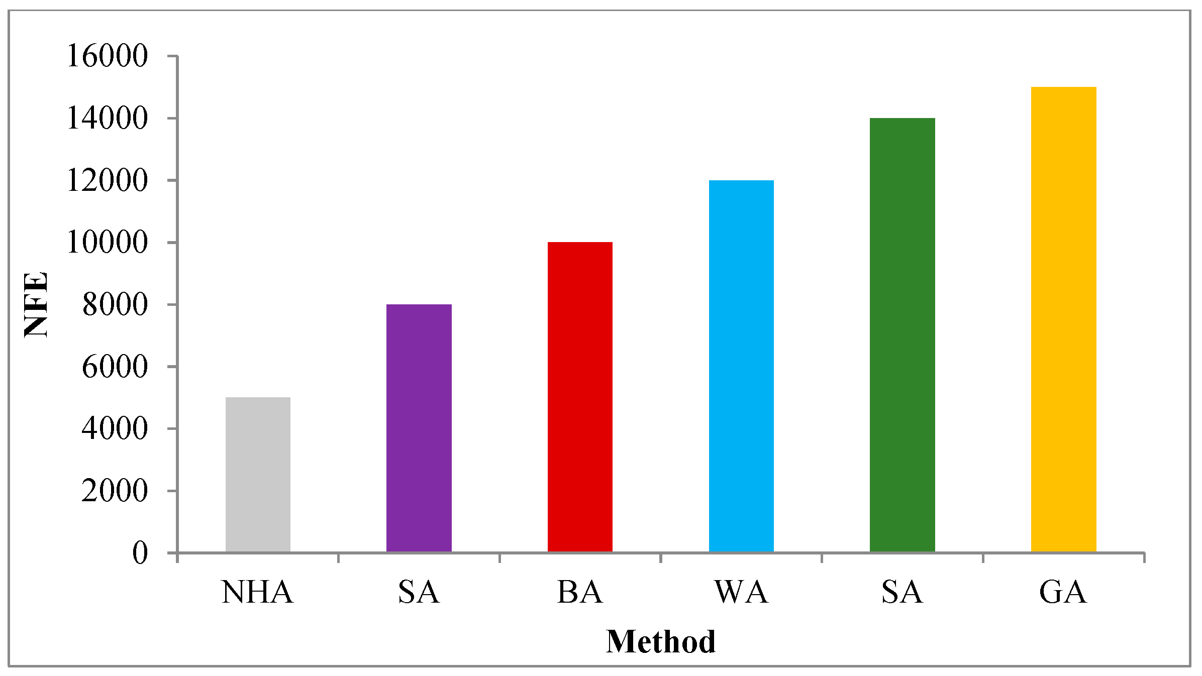
• Resiliency index. This index represents the existing speed of a system from failure. Thus, a high percentage for this index is preferable. This index shows the flexibility of different algorithms versus the critical periods when they should manage the system well [35].

  $${\gamma }_i=\frac{f_{si}}{F_i},$$

  (35)

  where ${\gamma }_i$ is the resiliency index; f_si is the number of failure series that occurred; and $F_i$ is the number of failure periods that occurred. These indexes were used to evaluate the percentage of success of the examined optimization algorithms based on their achieved operation rules to minimize the gap between the water release and water demand. Furthermore, to evaluate the performance of each algorithm with respect to the computational time needed for convergence, the time consumption for each algorithm to achieve the operation rule was determined. The best algorithm is the one that could achieve the global optima in less time for convergence.

5. Results, Discussion, and Application Analysis

5.1. Benchmark Functions

The standard deviation (SD), mean error (ME), average number of function evaluations (ANFE), and success rate (SR) are used to compare the results achieved from each algorithm for each benchmark function as shown in

Table 3. Experimental results using benchmark functions. SD—standard deviation; ME—mean error; ANFE—average number of function evaluations; SR—success rate; NHA—new hybrid algorithm.

Function	Algorithms	SD	ME	ANFE	SR
f1	Differential Evolution Algorithm	1.42 × 10−4 [52]	8.68 × 10−4 [52]	27,378 [52]	100
	Artificial Bee Colony Algorithm	2.02 × 10−4 [52]	7.54 × 10−4 [52]	35,091 [52]	100
	Particle Swarm Optimization	6.72 × 10−5	9.34 × 10−4	45,914.5	100
	Bat Algorithm	5.12 × 10−5	6.12 × 10−4	231,245	100
	Shark Algorithm	5.01 × 10−5	5.25 × 10−4	209,878	100
	Genetic Algorithm	1.34 × 10−5	9.56 × 10−4	37,094	100
	Spider Monkey Algorithm	2.12 × 10−6 [52]	5.65 × 10−5	19,878 [52]	100
	Krill Algorithm	2.22 × 10−6 [52]	7.12 × 10−5	18,235 [52]	100
	NHA	5.25 × 10−7	8.12 × 10−6	14,224	100
f2	Differential Evolution Algorithm	4.93 [52]	2.09 × 10−3 [53]	200,000 [52]	98
	Artificial Bee Colony Algorithm	3.14 × 10−4 [52]	7.48 × 10−4 [53]	87,039 [52]	98
	Particle Swarm Optimization	1.35 × 10+1	2.98 × 10−3	200,000	98
	Bat Algorithm	3.24 × 10−5	3.12 × 10−5	54,223	98
	Shark Algorithm	4.56 × 10−7	4.12 × 10−6	45,221	98
	Genetic Algorithm	8.78	2.12 × 10−3	205,000	98
	Spider Monkey Algorithm	6.12 × 10−8 [53]	5.12 × 10−7 [53]	32,124 [53]	98
	Krill Algorithm	7.91 × 10−7 [53]	6.12 × 10−7 [53]	35,125 [53]	100
	NHA	9.12 × 10−9	7.12 × 10−8	310,191	100
f3	Differential Evolution Algorithm	1.12 × 10−3	4.09 × 10−1	2725.5	100
	Artificial Bee Colony Algorithm	5.25 × 10−3	4.09 × 10−1	2567	85
	Particle Swarm Optimization	5.64 × 10−3	4.02 × 10−1	4979	85
	Bat Algorithm	4.12 × 10−4	3.12 × 10−2	1285	85
	Shark Algorithm	5.12 × 10−5	3.22 × 10−2	1100	98
	Genetic Algorithm	1.12 × 10−2	4.12 × 10+1	1400	98
	Spider Monkey Algorithm	5.78 × 10−5	2.12 × 10−4	987	98
	Krill Algorithm	5.45 × 10−3	3.12 × 10−5	765	98
	NHA	1.14 × 10−6	1.12 × 10−6	654	100
f4	Differential Evolution Algorithm	1.12 × 10+2	2.19 × 10+1	180,000	84
	Artificial Bee Colony Algorithm	1.18 × 10+1	1.19 × 10+1	170,000	84
	Particle Swarm Optimization	6.70 × 10+2	2.80 × 10−3	200,000	84
	Bat Algorithm	5.70 × 10−3	1.12 × 10−4	180,000	84
	Shark Algorithm	4.71 × 10−3	5.45 × 10−5	160,000	84
	Genetic Algorithm	6.14 × 10+3	1.21 × 10−2	210,000	84
	Spider Monkey Algorithm	1.45 × 10−4	3.12 × 10−5	180,000	84
	Krill Algorithm	1.23 × 10−5	4.21 × 10−5	165,000	84
	NHA	2.12 × 10−6	2.12 × 10−7	140,000	98
f5	Differential Evolution Algorithm	1.31 × 10−6	4.90 × 10−1	2741	100
	Artificial Bee Colony Algorithm	2.00 × 10−6	4.87 × 10−1	4811	100
	Particle Swarm Optimization	6.12 × 10−7	4.75 × 10−1	4912	100
	Bat Algorithm	2.12 × 10−8	2.22 × 10−3	1811	100
	Shark Algorithm	1.11 × 10−8	2.12 × 10−4	1712	100
	Genetic Algorithm	1.21 × 10−5	3.21 × 10−4	5121	100
	Spider Monkey Algorithm	2.12 × 10−8	5.12 × 10−3	1001	100
	Krill Algorithm	1.14 × 10−8	5.45 × 10−4	987	100
	NHA	1.41 × 10−9	6.78 × 10−5	567	100

. The ANFE is used as the average of the function evaluations that should be considered to obtain the termination criteria for 100 runs. The main purpose for including several indexes is the possibility of having biased results, which occurs when using a single index. For example, a particular algorithm might achieve the best value using a certain index, suggesting that this algorithm has the best potential to achieve the best results, whereas the same algorithm might fail when examined using another index. The results indicated that the NHA outperforms other methods when examined using all indexes. In addition, the statistical Mann–Whitney rank sum test is applied to evaluate the average function of 100 runs performed by two different methods, and it indicates whether one method is superior to the other. If the NHA is not significantly better than the other methods, the null hypothesis is supported; otherwise, the null hypothesis is rejected and the two methods are compared with each other. The results show that the NHA could outperform other methods based on statistical tests and different indexes. The parameters for the algorithms were obtained by the sensitivity analysis and the methods are in the reference [52].

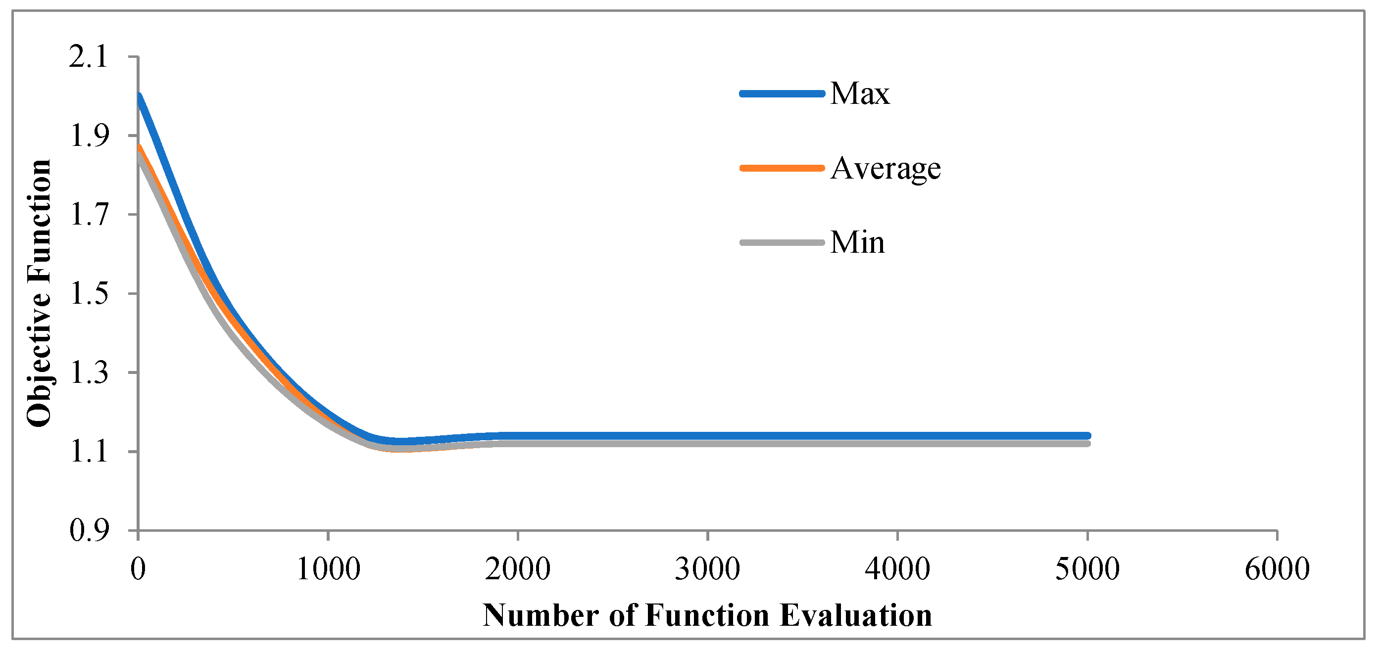
5.2. Sensitivity Analysis for the NHA

There are two main sources of uncertainty in this application; one is related to the optimization algorithm itself, and the other is related to the nature of the inputs and outputs of the case study. The uncertainty related to the optimization algorithm involves the initial parameters needed to initialize the model. The uncertainty related to the case study is based on the historical reservoir inflow records and water loss calculations from the reservoir due to evaporation and the release of water from the reservoir.

Table 4. Details of the sensitivity analysis for the new hybrid algorithm.

Size Population	Objective Function	W (Inertia Coefficient)	Objective Function	c1 = c2	Objective Function	Maximum Frequency	Objective Function	Minimum Loudness	Objective Function
10	2.45	0.30	2.21	1.6	2.34	1	2.11	0.3	2.23
30	2.24	0.50	2.00	1.8	2.12	2	2.00	0.5	2.05
50	1.98	0.70	1.98	2.0	1.98	3	2.14	0.7	2.0
70	2.01	0.90	2.12	2.2	2.12	4	2.16	0.90	2.1

,

Table 5. Details of the sensitivity analysis for the shark algorithm.

Size Population	Objective Function	βk (Velocity Limiter)	Objective Function	αk	Objective Function
10	2.45	2	2.44	0.20	2.55
30	2.12	4	2.12	0.40	2.12
50	2.24	6	2.34	0.60	2.67
70	2.36	8	2.44	0.80	2.78

,

Table 6. Details of the sensitivity analysis for the weed algorithm.

Pinitial	Objective Function	Pmax	Objective Function	N0Smax	Objective Function
5	3.69	10	3.55	3	3.78
10	3.12	30	3.12	5	3.34
15	3.24	50	3.28	7	3.12
20	3.36	70	3.32	9	3.44

and

Table 7. Details of the sensitivity analysis for the genetic algorithm.

Size Population	Objective Function	Mutation Probability	Objective Function	Crossover Probability	Objective Function
10	5.12	0.30	4.88	0.20	4.69
30	4.98	0.50	4.55	0.40	4.34
50	4.15	0.70	4.15	0.60	4.12
70	4.55	0.90	4.24	0.80	4.24

show the details of the sensitivity analysis for the proposed and comparable evolutionary algorithms. The sensitivity analysis shows the accuracy values of the random parameters obtained based on the variation in the value of the objective function versus the variation in the values of the random parameters. The size of the population for the NHA is 50 because the objective function has the smallest value (1.98). The maximum frequency for the NHA is 7 Hz, while the minimum frequency is 2 Hz. The acceleration coefficients (c₁ = c₂) are equal to 2, and the inertia weight is 0.7. Other accurate values for the other algorithms can be seen in Table 5, Table 6, Table 7 and

Table 8. Ten random results for the proposed hybrid evolutionary algorithm and the stand-alone algorithms.

Run	NHA	SA	BA	WA	PSO	GA
1	1.99	2.12	2.45	3.16	3.45	4.15
2	1.98	2.12	2.47	3.12	3.51	4.24
3	1.98	2.12	2.49	3.12	3.45	4.26
4	1.98	2.12	2.45	3.12	3.45	4.15
5	1.98	2.14	2.45	3.12	3.45	4.15
6	1.98	2.12	2.45	3.12	3.45	4.15
7	1.98	2.12	2.45	3.12	3.45	4.15
8	1.98	2.12	2.45	3.12	3.45	4.15
9	1.98	2.12	2.45	3.12	3.45	4.15
10	1.98	2.12	2.45	3.12	3.45	4.15
Average solution	1.98	2.12	2.45	3.12	3.45	4.17
Coefficient variation	0.001	0.002	0.005	0.004	0.005	0.006
Time	50	70	79	83	91	94

. The population size for the SA is 30, and the velocity limit for this method is 4. The mutation and crossover probabilities are 0.70 and 0.60, respectively. The size populations for P_initial and P_max based on the WA are 10 and 30, respectively. Additionally, other parameters can be seen in Table 5, Table 6 and Table 7.

5.3. Ten Random Results for Evolutionary Algorithms

Table 8 shows the ten random run results for different algorithms for the same year. The average solution attained using the NHA is 1.98, which is the lowest value among the other algorithms. The average solutions for the SA, BA, WA, PSO algorithm, and GA are 2.12, 2.45, 3.12, 3.45, and 4.15, respectively. On the basis of the achieved results, the NHA minimized the objective function better than the other algorithms. The computational time for the NHA is 50 s, whereas it is 70, 79, 83, 91, and 94 s for the SA, WA, BA, PSO algorithm, and GA, respectively. Accordingly, compared with the SA, BA, WA, PSO algorithm, and GA, the NHA decreased the computation time by 28%, 36%, 39%, 82%, and 88%, respectively, which is an excellent enhancement result.

The variation coefficient for the NHA model is less than that of the commensurate models (i.e., SA, BA, WA, PSO algorithm, and GA). The NHA displayed a reliable outcome based on the average; however, the average results have small variation coefficients, which can be seen in Figure 7, where the average, minimum, and maximum solutions overlap with each other and are well matched. Figure 8 shows the value of the objective function belonging to all data-intelligence models versus the number of function evaluations (NFEs). The NFE for the NHA model is equal to 5000. The other established models have NFE values of 8000, 1000, 12,000, 14,000, and 15,000 (SA, BA, WA, GA, and PSO algorithm, respectively). Thus, the NHA can obtain the best solutions with a smaller NFE, which shows that the NHA can obtain the converged solution faster than other algorithms.

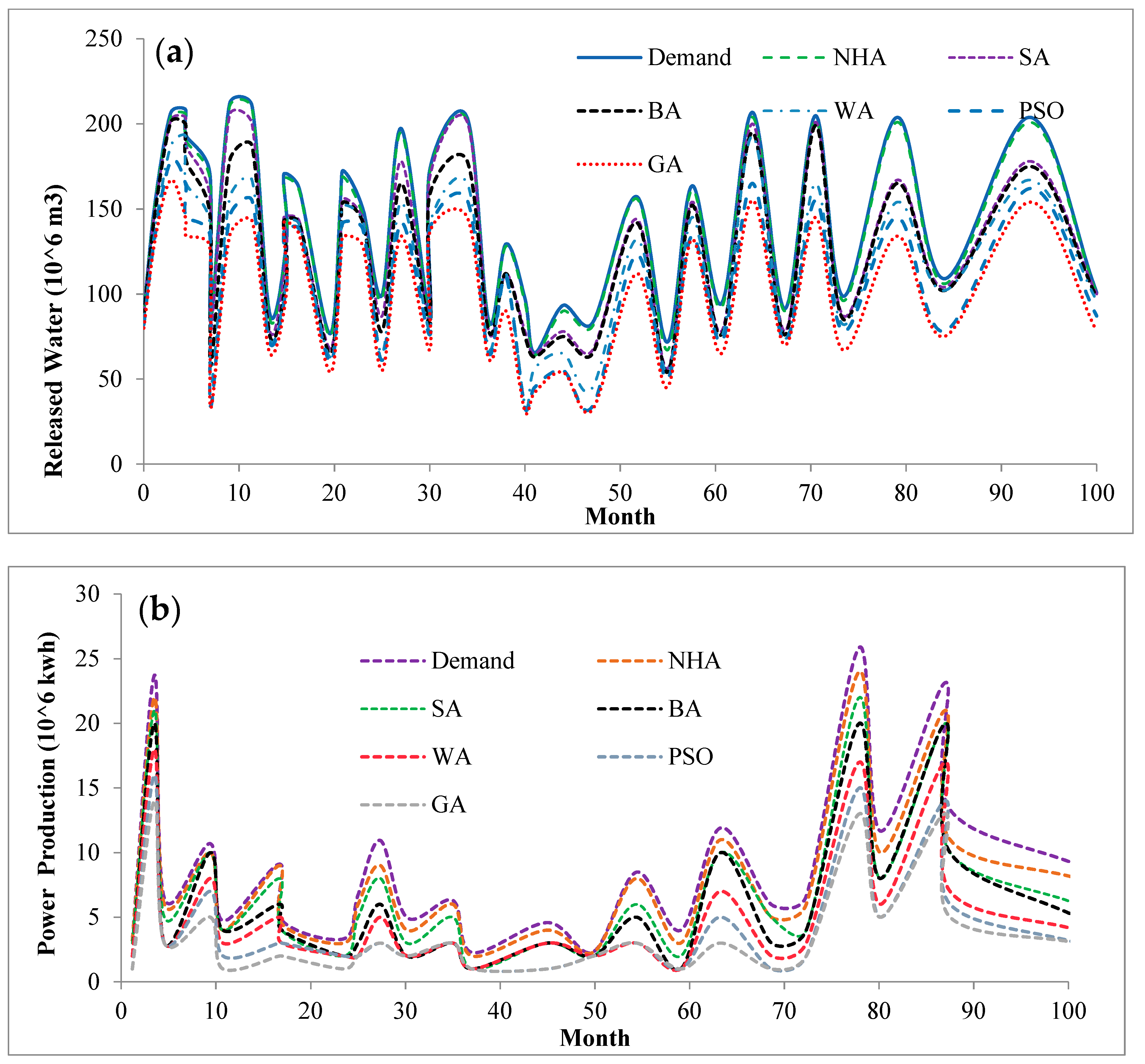
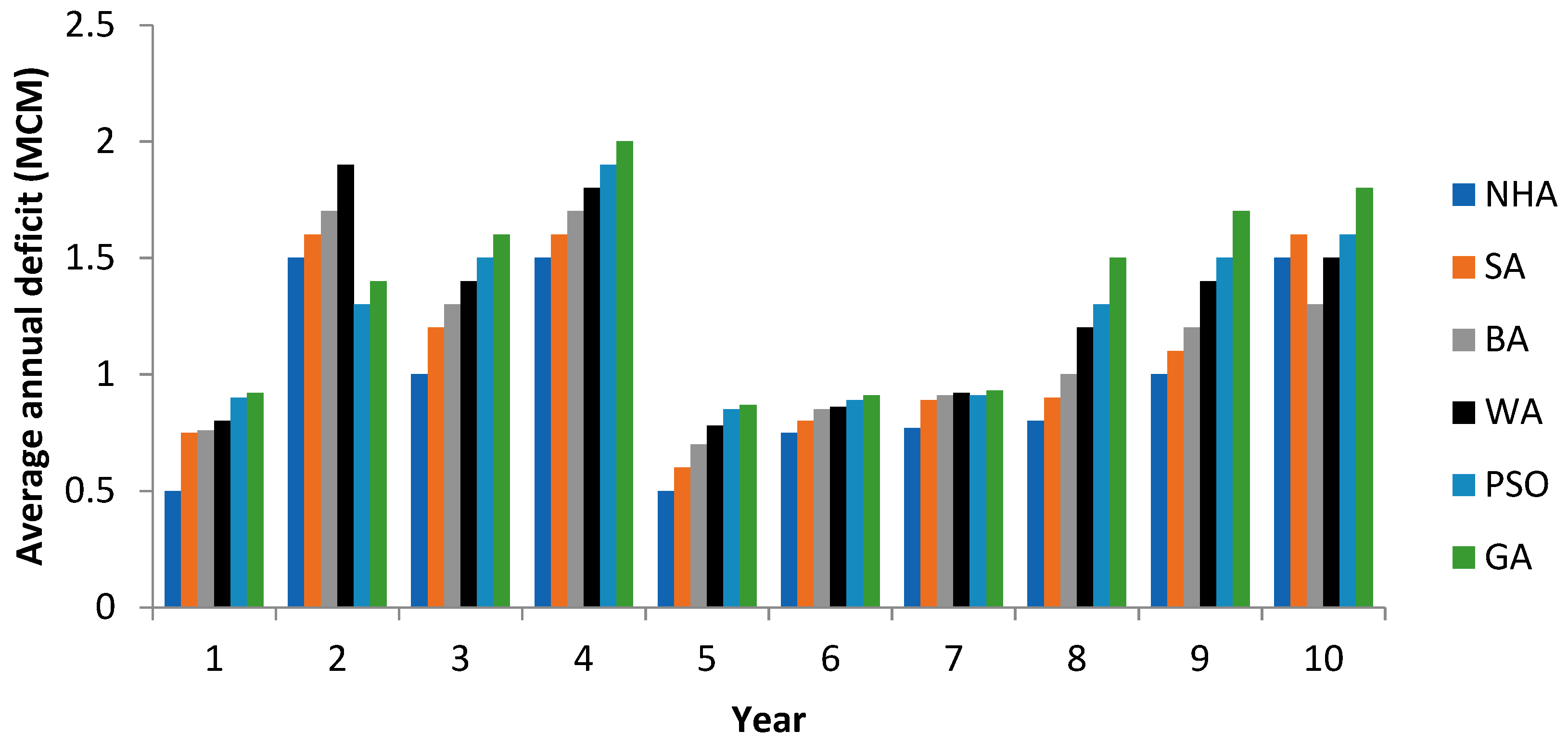
5.4. Computed Irrigation Deficiencies

Different indexes were used to evaluate the irrigation deficiencies tabulated in

Table 9. Evaluation of different algorithms for irrigation demands based on different indexes. NHA—new hybrid algorithm; SA—shark algorithm; BA—bat algorithm; WA—weed algorithm; PSO—particle swarm optimization; GA—genetic algorithm; MOGA—multi-objective GA; MOPSO—multi-objective PSO.

Index	Equation	NHA	SA	BA	WA	PSO	GA	MOGA	MOPSO
Correlation Coefficient	$r=\frac{{\displaystyle \sum _{t=1}^T\left(D_t-{\overline{D}}_t\right).\left(R_t-{\overline{R}}_t\right)}}{\sqrt{{\displaystyle \sum _{t=1}^T{\left(D_t-{\overline{D}}_t\right)}^2.{\displaystyle \sum _{t=1}^T\left(R_t-{\overline{R}}_t\right)}}}}$	0.93	0.91	0.86	0.87	0.75	0.67	0.74	0.83
Root Mean Square Error (RMSE) (106 m3)	$RMSE=\sqrt{\frac{{\displaystyle \sum _{t=1}^T{\left(D_t-R_t\right)}^2}}{T}}$	5.1	7.2	8.8	9.3	10.5	11.8	9.6	8.7
Mean absolute Error (106 m3)	$MAE=\frac{{\displaystyle \sum _{t=1}^T\left|D_t-R_t\right|}}{T}$	4.3	5.59	6.1	7.1	6.9	6.4	6.3	6.1
Volumetric Reliability Index%	${\alpha }_V=\frac{{\displaystyle \sum _{t=1}^T{R}_t}}{{\displaystyle \sum _{t=1}^T{D}_t}}\times 100$	95%	90%	87%	78%	75%	64%	77%	79%
Resiliency Index%	${\gamma }_i=\frac{f_{si}}{F_i}$	45%	40%	38%	35%	33%	29%	35%	34%
Vulnerability Index	$\lambda =Ma{x}_{t=1}^T\left(\frac{D_t-R_t}{D_t}\right)\times 100$	14%	20%	21%	23%	24%	25%	22%	21%

D_t: demand; ${\overline{D}}_t$: average demand; R_t: released water; and ${\overline{R}}_t$: average released water.

. The highest correlation attained for the proposed model had a magnitude of 0.93. Additionally, the absolute error metric values (e.g., the mean absolute error (MAE) and root mean square error (RMSE)) prove that released water can supply the irrigation demand for the left and right canals based on a smaller error index value and greater correlation value. The SA attained an accurate level of modelling after the use of the proposed hybrid model. Figure 9 shows the mode of the irrigation supply for all applied algorithms. The average demand for the total operation period is 142.14 (10⁶ m³), and the average amounts of released water for the NHA, SA, BA, WA, PSO algorithm and GA are 141.25, 140.33, 138.75, 135.43, 134.12 and 133.21 (10⁶ m³), respectively. Thus, the NHA can supply the irrigation demand as a primary priority in this problem. The volumetric reliability, vulnerability and resiliency indexes were used for more detailed information and a deep comparative analysis of all implemented algorithms. The high percentage for the volumetric reliability index found for the NHA showed that irrigation demands can be supplied for more operation periods; therefore, the volume of released water can respond to downstream irrigation demands. In fact, the volumetric reliability index based on the NHA is 5%, 8%, 17%, 18% and 31% greater than that based on the SA, BA, WA, PSO algorithm and GA, respectively.

Additionally, Reddy and Kumar [53] optimized this system based on the multi-objective GA (MOGA) and multi-objective PSO (MOPSO) algorithms. These multi-objective algorithms can be considered substitution strategies instead of weighting methods, and the structure and preparation of such algorithms are complex. The results indicated that the NHA has a better performance than the MOGA and the MOPSO algorithm; therefore, the volumetric reliability index for the NHA is greater than that for the MOGA and the MOPSO algorithms. For example, the Pareto fronts are shown in Figure 10. The marginal rate of substitution strategy [54] is used to select the best solution. The marginal rate of substitution can be calculated based on sacrificing certain terms of the objective function to improve the value of the other terms of the objective function. When one solution has the maximum value of marginal rate of substitution, it is the most suitable solution; in other words, the best solution has the highest slope for two objective functions in the Pareto front. When the MOGA and the MOPSO algorithm are used, a large number of solutions can be observed; thus, the problem must be simplified. Therefore, a simple clustering strategy is used to filter 200 solutions to 20 solutions. First, there are N clusters, and the cluster ranges are calculated for all pairs of clusters; then, each two clusters with the minimum range are combined to generate the large cluster. Finally, the solutions with the minimum average distance from other solutions in the cluster are considered as alternative solutions for clustering (Figure 10). The determined point blue is the optimal solution.

The vulnerability index for the NHA was 12%, which was the lowest percentage among the analyzed methods. The maximum intensity of the failure probability occurred with the NHA and was less than that of other evolutionary algorithms. The greatest value of the vulnerability index was related to the GA. Additionally, the NHA had a better performance than the MOGA and the MOPSO algorithms based on the lower value of the vulnerability index.

Finally, the resiliency index of the NHA was 45%, which was the highest percentage among the analysed methods; therefore, the multi-purpose system can escape more quickly from critical periods, such as drought periods.

Figure 11 shows that the NHA has the smallest average annual deficit among the evaluated methods. The average annual deficit for the NHA is 10%, 12%, 15%, 17%, and 18% less than that for the SA, BA, WA, PSO algorithm, and GA, respectively. The historical water demand required for various uses was recorded during an earlier time period, whereas the released water decision pattern was calculated based on the achieved optimal operation rules from each algorithm based on objective functions. Finally, a comparative analysis was carried out to identify the gap between the water demand for the irrigation requirement and power production and the allocated water release. The released water as a decision variable was calculated, and then the power generation was calculated based on released water; the resulting power produced was 106 kWh, which was then compared with the actual power required for downstream demands.

5.5. Computational Power Production

The downstream demand for power is 18.90 (10⁶ kwh), and the average amount of produced power based on the NHA is 18.08 (10⁶ kwh), while it is 17.99, 17.32, 16.96, 16.32, and 15.34 (10⁶ kwh) for the SA, BA, WA, PSO algorithm, and GA, respectively (see Figure 6b). Thus, the NHA can produce more power to supply the demand (

Table 10. Evaluation of different algorithms for irrigation demands based on different indexes.

Index	Equation	NHA	SA	BA	WA	PSO	GA	MOGA (Reddy, 2006)	MOPSO (Reddy, 2006)
Correlation Coefficient	$r=\frac{{\displaystyle \sum _{t=1}^T\left(P_{dt}-{\overline{P}}_{dt}\right).\left(P_{st}-{\overline{P}}_{st}\right)}}{\sqrt{{\displaystyle \sum _{t=1}^T{\left(P_{dt}-{\overline{P}}_{obt}\right)}^2.{\displaystyle \sum _{t=1}^T\left(P_{st}-{\overline{P}}_{st}\right)}}}}$	93%	90%	87%	75%	69%	65%	73%	75%
Root Mean Square Error (RMSE) (106 kwh)	$RMSE=\sqrt{\frac{{\displaystyle \sum _{t=1}^T{\left(P_{obt}-P_{st}\right)}^2}}{T}}$	3.1	4.9	4.2	3.8	4.2	3.7	3.5	3.8
Mean Absolute Error (MAE) (106 kwh)	$MAE=\frac{{\displaystyle \sum _{t=1}^T\left|P_{obt}-P_{st}\right|}}{T}$	3.2	4.1	3.8	3.6	3.4	3.5	3.3	3.4

$P_{dt}$: power demand; ${\overline{P}}_{dt}$: average power demand; and $P_{st}$: simulated produced power by algorithms.

). Additionally, the correlation coefficient for the NHA is greater than that for other algorithms, and the root mean square error (RMSE) and mean absolute error (MAE) have the smallest values in the NHA among the evaluated algorithms based on the difference between demand and power production. Additionally, the NHA has a better performance than the MOGA and the MOPSO algorithms based on the lower values for the error indexes and higher correlation values.

Thus, the NHA can supply the irrigation demand first; then, the power production can be used after the irrigation supply. Additionally, although the release of more water may generate more power, a considerable deficiency in irrigation would result. Thus, more weight is assigned to the irrigation objective function to ensure that the demand for irrigation is met; ensuring the necessary power production is an additional concern for policymakers.

6. Conclusions

The current research is dedicated to the implementation of a new hybrid intelligence model based on integrating two meta-heuristic algorithms for optimizing the operation of a multi-purpose reservoir water system. The optimization problem is solved to satisfy irrigation demands and hydropower production for one case study in India. The capability of the BA is improved by hybridization with the PSO algorithm based on local and global search strategies and the substitution of weaker solutions in each algorithm with the best solutions of the other algorithms. The main idea behind the procedure of the proposed NHA is to avoid the possible worst solutions using the BA and the resulting decline in local optima; in addition, the NHA enhanced the convergence rate using the PSO algorithm.

After applying the proposed NHA for a multi-purpose reservoir water system, namely the Bhadra Dam in India, it could be concluded that the NHA could provide a satisfactory improvement to decreasing irrigation deficiencies. In quantitative terms, the average irrigation demand was 142.14 (10⁶ m³), and the NHA can release 141.25 (10⁶ m³), which represents a much higher level of accuracy over comparable models. The average demand for power production is 18.08 (10⁶ kwh), and the produced power using the NHA is 17.99 (10⁶ kwh), which represents the capability of the NHA for applied applications.

It can be concluded that the proposed NHA as an intelligent model could contribute to providing reliable solutions for complex multi-purpose reservoir systems to optimize the operation rule for similar reservoir systems worldwide. In addition, the NHA could be integrated with other forecasting models for additional reservoir hydrological variables to optimize its operation under different climate change scenarios in future periods. Furthermore, the NHA could be used for multi-purpose reservoir systems and other multi-purpose engineering optimization applications.

Although the proposed NHA showed superior performance over the other optimization algorithms, it still experienced a challenge during initialization because several random parameters must be initialized. This step may prolong the computational time for convergence. In addition to the need to initialize the random parameters for the BA and PSO algorithms within the definition of the NHA communication, a simultaneous procedure must also be adopted to update these random parameters within the simulation model of the reservoir, and such requirements should be considered when applying the NHA to other case studies.

References

1. Pedro-Monzonís, M.; Solera, A.; Ferrer, J.; Estrela, T.; Paredes-Arquiola, J. A review of water scarcity and drought indexes in water resources planning and management. J. Hydrol. 2015, 527, 482–493. [Google Scholar] [CrossRef]
2. You, J.Y.; Cai, X. Hedging rule for reservoir operations: 2. A numerical model. Water Resour. Res. 2008, 44. [Google Scholar] [CrossRef]
3. Fang, H.; Hu, T.; Zeng, X.; Wu, F. Simulation-optimization model of reservoir operation based on target storage curves. Water Sci. Eng. 2014, 7, 433–445. [Google Scholar] [CrossRef]
4. Srinivasan, K.; Kumar, K. Multi-Objective Simulation-Optimization Model for Long-term Reservoir Operation using Piecewise Linear Hedging Rule. Water Resour. Manag. 2018, 32, 1901–1911. [Google Scholar] [CrossRef]
5. Xie, A.; Liu, P.; Guo, S.; Zhang, X.; Jiang, H.; Yang, G. Optimal Design of Seasonal Flood Limited Water Levels by Jointing Operation of the Reservoir and Floodplains. Water Resour. Manag. 2017, 32, 179–193. [Google Scholar] [CrossRef]
6. Adeyemo, J.A. Reservoir operation using multi-objective evolutionary algorithms—A review. Asian J. Sci. Res. 2011, 4, 16–27. [Google Scholar] [CrossRef]
7. Karamouz, M.; Nazif, S.; Sherafat, M.A.; Zahmatkesh, Z. Development of an Optimal Reservoir Operation Scheme Using Extended Evolutionary Computing Algorithms Based on Conflict Resolution Approach: A Case Study. Water Resour. Manag. 2014, 28, 3539–3554. [Google Scholar] [CrossRef]
8. Azizipour, M.; Ghalenoei, V.; Afshar, M.H.; Solis, S.S. Optimal Operation of Hydropower Reservoir Systems Using Weed Optimization Algorithm. Water Resour. Manag. 2016, 30, 3995–4009. [Google Scholar] [CrossRef]
9. Han, C.; Zheng, B.; Qin, Y.; Ma, Y.; Yang, C.; Liu, Z.; Cao, W.; Chi, M. Impact of upstream river inputs and reservoir operation on phosphorus fractions in water-particulate phases in the Three Gorges Reservoir. Sci. Total Environ. 2018, 610–611, 1546–1556. [Google Scholar] [CrossRef]
10. Wan, W.; Guo, X.; Lei, X.; Jiang, Y.; Wang, H. A Novel Optimization Method for Multi-Reservoir Operation Policy Derivation in Complex Inter-Basin Water Transfer System. Water Resour. Manag. 2017, 32, 31–51. [Google Scholar] [CrossRef]
11. Moeini, R.; Babaei, M. Constrained improved particle swarm optimization algorithm for optimal operation of large scale reservoir: Proposing three approaches. Evol. Syst. 2017, 8, 287–301. [Google Scholar] [CrossRef]
12. Zyoud, S.H.; Kaufmann, L.G.; Shaheen, H.; Samhan, S.; Fuchs-Hanusch, D. A framework for water loss management in developing countries under fuzzy environment: Integration of Fuzzy AHP with Fuzzy TOPSIS. Expert Syst. Appl. 2016, 61, 86–105. [Google Scholar] [CrossRef]
13. Rabiei, M.; Aalami, M.; Talatahari, S. Reservoir Operation Optimization using CBO, ECBO and vps algorithms. Iran Univ. Sci. Technol. 2018, 8, 489–509. [Google Scholar]
14. Tayfur, G. Modern Optimization Methods in Water Resources Planning, Engineering and Management. Water Resour. Manag. 2017, 31, 3205–3233. [Google Scholar] [CrossRef]
15. Bennett, C.; Stewart, R.A.; Beal, C.D. ANN-based residential water end-use demand forecasting model. Expert Syst. Appl. 2013, 40, 1014–1023. [Google Scholar] [CrossRef]
16. Nabaei, A.; Hamian, M.; Parsaei, M.R.; Safdari, R.; Samad-Soltani, T.; Zarrabi, H.; Ghassemi, A. Topologies and performance of intelligent algorithms: A comprehensive review. Artif. Intell. Rev. 2016. [Google Scholar] [CrossRef]
17. Ethteram, M.; Mousavi, S.F.; Karami, H.; Farzin, S.; Deo, R.; Othman, F.B.; Chau, K.; Sarkamaryan, S.; Singh, V.P.; El-Shafie, A. Bat algorithm for dam–reservoir operation. Environ. Earth Sci. 2018, 77, 510. [Google Scholar] [CrossRef]
18. Ehteram, M.; Singh, V.; Karami, H.; Hosseini, K.; Dianatikhah, M.; Hossain, M.; Ming Fai, C.; El-Shafie, A. Irrigation Management Based on Reservoir Operation with an Improved Weed Algorithm. Water 2018, 10, 1267. [Google Scholar] [CrossRef]
19. Allawi, M.F.; Jaafar, O.; Mohamad Hamzah, F.; Ehteram, M.; Hossain, M.S.; El-Shafie, A. Operating a reservoir system based on the shark machine learning algorithm. Environ. Earth Sci. 2018, 77, 366. [Google Scholar] [CrossRef]
20. Allawi, M.F.; Jaafar, O.; Mohamad Hamzah, F.; Koting, S.B.; Mohd, N.S.B.; El-Shafie, A. Forecasting hydrological parameters for reservoir system utilizing artificial intelligent models and exploring their influence on operation performance. Knowl.-Based Syst. 2019, 163, 907–926. [Google Scholar] [CrossRef]
21. Raso, L.; Chiavico, M.; Dorchies, D. Optimal and Centralized Reservoir Management for Drought and Flood Protection on the Upper Seine–Aube River System Using Stochastic Dual Dynamic Programming. J. Water Resour. Plan. Manag. 2019, 145, 5019002. [Google Scholar] [CrossRef]
22. Allawi, M.F.; Jaafar, O.; Ehteram, M.; Mohamad Hamzah, F.; El-Shafie, A. Synchronizing Artificial Intelligence Models for Operating the Dam and Reservoir System. Water Resour. Manag. 2018, 32, 3373–3389. [Google Scholar] [CrossRef]
23. Ehteram, M.; Karami, H.; Farzin, S. Reservoir Optimization for Energy Production Using a New Evolutionary Algorithm Based on Multi-Criteria Decision-Making Models. Water Resour. Manag. 2018, 32, 2539–2560. [Google Scholar] [CrossRef]
24. Ehteram, M.; Mousavi, S.F.; Karami, H.; Farzin, S.; Emami, M.; Binti Othman, F.; Amini, Z.; Kisi, O.; El-Shafie, A. Fast convergence optimization model for single and multi-purposes reservoirs using hybrid algorithm. Adv. Eng. Inform. 2017, 32, 287–298. [Google Scholar] [CrossRef]
25. Afshar, A.; Shafii, M.; Haddad, O.B. Optimizing multi-reservoir operation rules: An improved HBMO approach. J. Hydroinform. 2010, 13, 121. [Google Scholar] [CrossRef]
26. Fallah-Mehdipour, E.; Bozorg Haddad, O.; Mariño, M.A. Real-Time Operation of Reservoir System by Genetic Programming. Water Resour. Manag. 2012, 26, 4091–4103. [Google Scholar] [CrossRef]
27. Ostadrahimi, L.; Mariño, M.A.; Afshar, A. Multi-reservoir Operation Rules: Multi-swarm PSO-based Optimization Approach. Water Resour. Manag. 2011, 26, 407–427. [Google Scholar] [CrossRef]
28. Bolouri-Yazdeli, Y.; Bozorg Haddad, O.; Fallah-Mehdipour, E.; Mariño, M.A. Evaluation of real-time operation rules in reservoir systems operation. Water Resour. Manag. 2014, 28, 715–729. [Google Scholar] [CrossRef]
29. Akbari-Alashti, H.; Bozorg Haddad, O.; Fallah-Mehdipour, E.; Mariño, M.A. Multi-reservoir real-time operation rules: A new genetic programming approach. Proc. Inst. Civ. Eng. Water Manag. 2014, 167, 561–576. [Google Scholar] [CrossRef]
30. Haddad, O.B.; Moravej, M.; Loáiciga, H.A. Application of the Water Cycle Algorithm to the Optimal Operation of Reservoir Systems. J. Irrig. Drain. Eng. 2015, 141, 04014064. [Google Scholar] [CrossRef]
31. Haddad, O.B.; Hosseini-Moghari, S.-M.; Loáiciga, H.A. Biogeography-Based Optimization Algorithm for Optimal Operation of Reservoir Systems. J. Water Resour. Plan. Manag. 2016, 142, 04015034. [Google Scholar] [CrossRef]
32. Zhang, Z.; Jiang, Y.; Zhang, S.; Geng, S.; Wang, H.; Sang, G. An adaptive particle swarm optimization algorithm for reservoir operation optimization. Appl. Soft Comput. J. 2014, 18, 167–177. [Google Scholar] [CrossRef]
33. Hosseini-Moghari, S.-M.; Morovati, R.; Moghadas, M.; Araghinejad, S. Optimum Operation of Reservoir Using Two Evolutionary Algorithms: Imperialist Competitive Algorithm (ICA) and Cuckoo Optimization Algorithm (COA). Water Resour. Manag. 2015, 29, 3749–3769. [Google Scholar] [CrossRef]
34. Ehteram, M.; Karami, H.; Mousavi, S.-F.; Farzin, S.; Kisi, O. Evaluation of contemporary evolutionary algorithms for optimization in reservoir operation and water supply. J. Water Supply Res. Technol. 2017, jws2017109. [Google Scholar] [CrossRef]
35. Ehteram, M.; Karami, H.; Mousavi, S.-F.; Farzin, S.; Kisi, O. Optimization of energy management and conversion in the multi-reservoir systems based on evolutionary algorithms. J. Clean. Prod. 2017, 168, 1132–1142. [Google Scholar] [CrossRef]
36. Garg, H. A hybrid GSA-GA algorithm for constrained optimization problems. Inf. Sci. 2019, 478, 499–523. [Google Scholar] [CrossRef]
37. Patwal, R.S.; Narang, N.; Garg, H. A novel TVAC-PSO based mutation strategies algorithm for generation scheduling of pumped storage hydrothermal system incorporating solar units. Energy 2018, 142, 822–837. [Google Scholar] [CrossRef]
38. Garg, H. A hybrid PSO-GA algorithm for constrained optimization problems. Appl. Math. Comput. 2016, 274, 292–305. [Google Scholar] [CrossRef]
39. Garg, H. An efficient biogeography based optimization algorithm for solving reliability optimization problems. Swarm Evol. Comput. 2015, 24, 1–10. [Google Scholar] [CrossRef]
40. Shah, H.; Tairan, N.; Garg, H.; Ghazali, R. Global Gbest Guided-Artificial Bee Colony Algorithm for Numerical Function Optimization. Computers 2018, 7, 69. [Google Scholar] [CrossRef]
41. Yang, X.S. Bat algorithm for multi-objective optimisation. Int. J. Bio-Inspired Comput. 2011, 3, 267. [Google Scholar] [CrossRef]
42. Gandomi, A.H.; Yang, X.S. Chaotic bat algorithm. J. Comput. Sci. 2014, 5, 224–232. [Google Scholar] [CrossRef]
43. Yang, X.S. A new metaheuristic Bat-inspired Algorithm. In Studies in Computational Intelligence; Springer: Berlin/Heidelberg, Germany, 2010; Volume 284, pp. 65–74. [Google Scholar]
44. Bozorg-Haddad, O.; Karimirad, I.; Seifollahi-Aghmiuni, S.; Loáiciga, H.A. Development and Application of the Bat Algorithm for Optimizing the Operation of Reservoir Systems. J. Water Resour. Plan. Manag. 2015, 141, 04014097. [Google Scholar] [CrossRef]
45. Wang, Y.Y.; Zhou, J.; Zhou, C.; Wang, Y.Y.; Qin, H.; Lu, Y. An improved self-adaptive PSO technique for short-term hydrothermal scheduling. Expert Syst. Appl. 2012, 39, 2288–2295. [Google Scholar] [CrossRef]
46. Karami, H.; Mousavi, S.F.; Farzin, S.; Ehteram, M.; Singh, V.P.; Kisi, O. Improved Krill Algorithm for Reservoir Operation. Water Resour. Manag. 2018, 32, 3353–3372. [Google Scholar] [CrossRef]
47. Li, L.; Zhou, Y. A novel complex-valued bat algorithm. Neural Comput. Appl. 2014, 25, 1369–1381. [Google Scholar] [CrossRef]
48. Kennedy, J.; Eberhart, R. Particle swarm optimization. Neural Netw. 1995, 4, 1942–1948. [Google Scholar] [CrossRef]
49. Ehteram, M.; Karami, H.; Farzin, S. Reducing Irrigation Deficiencies Based Optimizing Model for Multi-Reservoir Systems Utilizing Spider Monkey Algorithm. Water Resour. Manag. 2018, 32, 2315–2334. [Google Scholar] [CrossRef]
50. Mehrabian, A.R.; Lucas, C. A novel numerical optimization algorithm inspired from weed colonization. Ecol. Inform. 2006, 1, 355–366. [Google Scholar] [CrossRef]
51. Hersovici, M.; Jacovi, M.; Maarek, Y.S.; Pelleg, D.; Shtalhaim, M.; Ur, S. The shark-search algorithm. An application: Tailored Web site mapping. Comput. Netw. ISDN Syst. 1998, 30, 317–326. [Google Scholar] [CrossRef]
52. Bansal, J.C.; Sharma, H.; Jadon, S.S.; Clerc, M. Spider Monkey Optimization algorithm for numerical optimization. Memetic Comput. 2014, 6, 31–47. [Google Scholar] [CrossRef]
53. Reddy, M.J.; Kumar, D.N. Optimal reservoir operation using multi-objective evolutionary algorithm. Water Resour. Manag. 2006, 20, 861–878. [Google Scholar] [CrossRef]
54. Deb, K.; Zhu, L.; Kulkarni, S. Multi-scenario, multi-objective optimization using evolutionary algorithms: Initial results. In Proceedings of the 2015 IEEE Congress on Evolutionary Computation, Sendai, Japan, 25–28 May 2015; pp. 1877–1884. [Google Scholar]
Figure 1. Bat algorithm procedure (rnd: random number).
Sustainability 11 01953 g001
Figure 2. New hybrid algorithm (NHA) diagram of the hybridized particle swarm optimization (PSO)–bat algorithm (BA) with a communication strategy.
Sustainability 11 01953 g002
Figure 3. Levels of reproduction for each plant with respect to fitness.
Sustainability 11 01953 g003
Figure 4. Weed algorithm (WA) procedure.
Sustainability 11 01953 g004
Figure 5. Shark algorithm (SA) procedure.
Sustainability 11 01953 g005
Figure 6. (a) Schematic diagram of the Bhadra reservoir system; (b) location of basin.
Sustainability 11 01953 g006
Figure 7. Convergence curve for the maximum, minimum, and average solution.
Sustainability 11 01953 g007
Figure 8. Comparison of the fitness value and number of function evaluation (NFE) for different algorithms. GA—genetic algorithm.
Sustainability 11 01953 g008
Figure 9. (a) Released water for downstream irrigation and (b) power production for downstream demand.
Sustainability 11 01953 g009
Figure 10. Pareto front for the algorithms. MOGA—multi-objective GA; MOPSO—multi-objective PSO.
Sustainability 11 01953 g010
Figure 11. Average annual deficits for different algorithms.
Sustainability 11 01953 g011