Article

Methodology for the Optimal Design of a Hybrid Charging Station of Electric and Fuel Cell Vehicles Supplied by Renewable Energies and an Energy Storage System

by
Higinio Sánchez-Sáinz
1,
Carlos-Andrés García-Vázquez
2,
Francisco Llorens Iborra
2 and
Luis M. Fernández-Ramírez
2,*
1
Research Group in Electrical Technologies for Sustainable and Renewable Energy (PAIDI-TEP-023), Department of Electrical Engineering, ESI Puerto Real, University of Cádiz, Avda. Universidad de Cádiz, nº10, 11519 Puerto Real (Cádiz), Spain
2
Research Group in Electrical Technologies for Sustainable and Renewable Energy (PAIDI-TEP-023), Department of Electrical Engineering, University of Cádiz, EPS Algeciras, Avda. Ramón Puyol, s/n, 11202 Algeciras (Cádiz), Spain
*
Author to whom correspondence should be addressed.
Sustainability 2019, 11(20), 5743; https://doi.org/10.3390/su11205743
Submission received: 1 September 2019 / Revised: 7 October 2019 / Accepted: 15 October 2019 / Published: 17 October 2019
(This article belongs to the Special Issue Sustainable Hydrogen Energy Systems: Electric Applications)

Abstract

:
The global energy system is changing, mainly to achieve sustainable transport technologies and clean electrical generation based on renewable sources. Thus, as fuels, electricity and hydrogen are the most promising transport technologies in order to reduce greenhouse emissions. On the other hand, photovoltaic and wind energies, including energy storage, have become the main sources of distributed generation. This study proposes a new optimal-technical sizing method based on the Simulink Design Optimization of a stand-alone microgrid with renewable energy sources and energy storage to provide energy to a wireless power transfer system to charge electric vehicles along a motorway and to a hydrogen charging station for fuel cell-powered buses. The results show that the design system can provide energy for the charging of electric vehicles along the motorway and produce the hydrogen consumed by the fuel cell-buses plus a certain tank reserve. The flexibility of the study allows the analysis of other scenarios, design requirements, configurations or types of microgrids.

1. Introduction

Currently, the transportation industry is one of the main energy consumers. Taking the data provided by the EU expert group on future transport fuels as a reference [1], 31.8% of energy is consumed by transport. Road transport is by far the largest energy consumer (72.3% of the total). Of all fuels used in road transport, oil products (diesel, fuel oil, natural gas, biofuels, gasoline, liquefied petrol gas) account for 86.3%, and diesel is the most used. All of this shows the current energy dependence of transportation on oil-derived fuels. The main aspect to consider with these fuels is the greenhouse gas (GHG) emissions associated with most of them. These aspects justify the efforts to develop alternative solutions to the use of these fuels. It is also true that these types of fuels are running out.
The Energy–Economy–Environment Modelling Laboratory (E3M-Lab) [2] developed the PRIMES-TREMOVE transport model [3] for long-term energy–economic–environmental planning in the European Union. Several studies focusing on the evolution of the use of fuels in transport in the medium term were developed using this model. Assuming a 60% reduction objective of GHG emissions, one of these studies established that the use of both electricity and hydrogen as transportation fuels would reach 23.2% of the total for 2050 [1]. To achieve these goals, it is essential to consider the presence of electric vehicles (EVs), both those that use electricity as primary energy, such as battery electric vehicles (BEVs), plug-in hybrid electric vehicles and hybrid electric vehicles, and those powered by hydrogen, such as fuel cell electric vehicles (FCEVs).
The charging process of BEVs, which are considered the EVs with the lowest GHG emissions, is one of the tasks which poses the greatest technological challenge today. The type of charging most widely used today is based on plugging the vehicle into an outlet, meaning that the vehicle has to stand still while the charging takes place. In addition, this process can be extended from several tens of minutes to a few hours, depending on the charging speed. Wireless power transfer charging systems are an alternative for the charging of BEVs, since they allow charging without connecting the vehicle to the grid through a wire. These systems allow stationary or dynamic charging. The technological solutions for wireless power transfer used in EVs charging were studied in Reference [4]. The current status and future trends of this type of charging were analyzed in Reference [5]. Hence, works published about the dynamic charging of EVs are less common. The Korea Advanced Institute of Science and Technology has developed an online EV and innovative electric transportation system that uses a wireless power transfer system, whose design was presented in Reference [6], and an economic analysis was presented in Reference [7]. Oak Ridge National Laboratory described their experiences and challenges in the dynamic wireless charging of EV in Reference [8]. In Reference [9], the viability of dynamic wireless power transfer (DWPT) systems for the dynamic charging of EVs on England’s major roads was studied from several points of view. A comparative study of the dynamic wireless charging of EVs for different types of roads was presented in Reference [10]. This charging option was contemplated in the FABRIC project (feasibility analysis and development of on-road charging solutions for future EVs) [11], supported and co-funded by the European Union in the Seventh Framework Program and by EUCAR (European Council for Automotive R&D) and ERTICO-ITS Europe.
Using renewable energy to produce the electricity needed to charge EVs, whatever the type of recharging method used, could be an interesting option to reduce GHG emissions. In the recently published literature, some contributions have been found, such as in References [12,13], in which the respective authors propose different solutions to use solar arrays to power an EV charging system.
Regarding FCEVs, fuel cell-powered buses (FCB) for public transport have played a great role in research and development in recent times, and so they have become one of the alternatives to the use of conventional buses with internal combustion engines. The work published in Reference [14] compared the performance of five types of buses: conventional, hydrogen-based, electric-battery and electric-hybrid, using a well-to-wheel analysis. Among the conclusions, the authors stated that FCBs are the most competitive choice in the long term and for all types of uses. China is taking steps to use FCBs and to avoid the blight caused by internal combustion vehicles [15]. The sustainability of the use of FCBs in public transport in Europe was evaluated in Reference [16]. A model to evaluate the economic, environmental and social sustainability of a fleet of FCBs was proposed in Reference [17]. The model used three different analyses and provided results that show the negative and positive impacts of the project. The feasibility of using hydrogen as a fuel in public passenger transport was evaluated for 13 cases studies conducted for 12 different locations in the NewBusFuel project [18]. Despite the different local conditions, bus operators and national regulatory framework in each selected location, the major success of the project was the development of solutions for hydrogen refueling stations in each location. In all these solutions, components and technologies available today were used, which proved that there are no insurmountable limits related to hydrogen infrastructure.
Electric power and hydrogen have different production pathways. Electricity production from renewable energy sources has zero GHG emissions [19]. In hydrogen production from water electrolysis, nearly zero emissions are achieved, because the hydrogen is usually generated by electricity from the grid. If this production were performed with renewable energy sources, zero emissions could be achieved. Nevertheless, this procedure requires a great contribution of electrical energy, and it is only economically viable if the electricity prices used to produce hydrogen are low. One of the options for producing electricity at low prices is by using renewable energy sources. The main factors against renewable electricity production are the geographical dependence of renewable sources and their variability. The use of energy storage systems is a feasible way to reduce the intermittency, unpredictability and fluctuations of renewable electricity production. If there is enough renewable energy available, a stand-alone microgrid combining renewable energy sources, usually wind energy and photovoltaic (PV) solar energy and energy storage devices, represents an interesting option to produce, with the lowest GHG, the electrical energy required by EVs [1].
Obviously, the correct sizing of the stand-alone microgrid is a primary task to ensure that it can meet energy demand. A review of size optimization methodologies for stand-alone renewable energy-based microgrid (REM) based on PV solar and wind energy was presented in Reference [20]. In this work, different configurations of stand-alone REM were analyzed, combining wind turbine (WT) and PV systems, with and without energy storage, and with the support of other conventional and/or renewable energy sources. The reliability, economy, environment or social criteria of the REM were studied. Stand-alone hybrid renewable energy systems are used in most cases for rural electrification [21], remote areas [22] or residential applications [23,24,25]. Nevertheless, to the best of our knowledge, no papers have been produced in which a stand-alone hybrid renewable energy system or microgrid for a hybrid charging station was sized and studied, which is the main objective of this work.
The optimization techniques analyzed in Reference [20] were divided into three large groups. The first group included techniques called classical techniques, such as linear programming (LP) [26], mixed-integer linear programming (MILP) [27], or those based on analytical methods [28]. The second group included the modern or artificial techniques: these include techniques such as genetic algorithms (GA) [29], mine blast algorithm (MBA) [30], particle swarm optimization (PSO) [31], multi-objective line-up competition algorithm (MLUC) [32], colony optimization (CO) [33] and others. The third were those that use hybrid algorithms, such as hybrid big bang-big crunch (HBB-BC) [34], teaching–learning-based optimization algorithm (TLBO) [35], iterative-Pareto-fuzzy (IPF) [36] and others. Finally, the third group includes computer software tools, such as HOMER/HOMER Pro [37] or iHOGA [38].
Computational calculation tools in general, and particularly HOMER/HOMER Pro, have become one of the most used alternatives in the recent literature on REM sizing [39,40]. One of the main advantages offered by HOMER is that its use does not require deep knowledge about optimization techniques from the user, which has made its use generalized, both in research and in applied engineering studies. On the other hand, HOMER clearly has four major disadvantages. The first is that the elements that appear in the microgrid under study must be adapted to the options offered by the software. It is not possible to choose different models for the elements, and although the offer of available equipment is wide, it is not possible to include equipment that is not implemented. The second major disadvantage is the inability to choose the optimization method used in sizing. The third major disadvantage is that it only allows a single-objective optimization by minimizing the total net present cost (NPC), and the last one is the impossibility of considering a specific control strategy defined by the user.
Among all existing optimization methods and tools, we chose to use the Simulink Design Optimization (SDO) [41]. SDO is an add-on of Simulink [42] that provides functions, interactive tools, and blocks for analyzing and tuning model parameters. The use of SDO for REM size optimization offers significant advantages over the computational tools indicated above. In SDO, the modeling of each component of the microgrid must be performed in Simulink. This allows users to choose the most appropriate model of each element of the microgrid. It is possible to include any type of element in the microgrid, provided that a Simulink model is available, and to implement any control strategy defined by the user depending on the control desired for the microgrid. Regarding the optimization method used, it should be noted that it is not unique; it can be chosen among several methods available in the MATLAB Optimization Toolbox. The choice and application of the optimization algorithm to the Simulink model is done in SDO by a Graphical User Interface. This allows it to be used by users without deep optimization knowledge. Finally, depending on how the model is defined in Simulink, the application of SDO allows the implementation of multi-objective optimization, which can be based on technical, economic, or technical–economic criteria. In the recent literature, there are not many papers which use SDO, however, when SDO is used, it is applied in two areas: the optimal setting of controllers and the optimal sizing of stand-alone microgrids [43,44,45]. Three papers on this topic were developed by the authors of the work presented here.
The main contributions of this work are the following: (1) the optimal sizing of a stand-alone microgrid for a hybrid charging station of electric and fuel cell vehicles was studied for the first time in the literature; and (2) the use of MATLAB-Simulink for the implementation of the dynamic model and control of the microgrid, and SDO for the optimal sizing of the microgrid, which offered great simplicity and flexibility for the design and evaluation of the microgrid under different scenarios and design requirements.
The remainder of the paper is divided as follows. Section 2 presents the microgrid under study. The basic characteristics of the considered DWPT system are explained in Section 3. Section 4 describes the fleet of FCBs under study, and evaluates the hydrogen refueling required by the fleet and energy requirements for the hydrogen production. The model of the microgrid and the procedure based on SDO for the optimal sizing of the microgrid are detailed in Section 5. Section 6 presents the results obtained for the different sizing carried out, as well as the verification and discussion of results. Finally, Section 7 presents the conclusions that can be derived from this work.

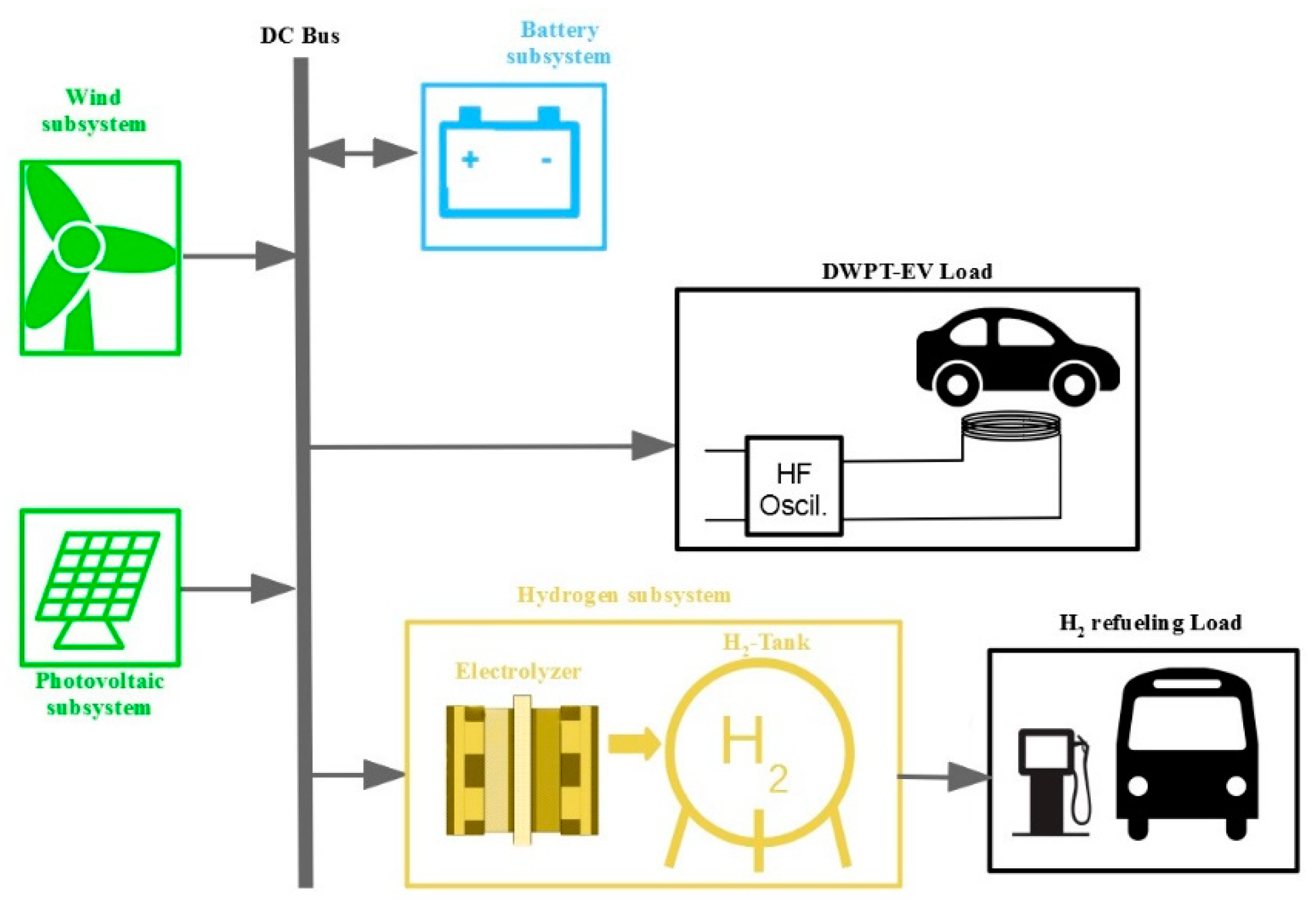
2. Microgrid under Study

This paper proposes the optimal sizing and evaluation of a stand-alone microgrid to supply long-term electricity to a wireless power transfer system for the dynamic charging of EVs and a hydrogen charging station for FCBs. The configuration of the microgrid under study is shown in Figure 1. The sizing of both subsystems affected the whole system sizing.
In the microgrid, WTs and PV panels acted as primary energy sources producing electricity. A battery energy storage system was used to store surplus energy in the hours for which the production was greater than the consumption. On the other hand, when the energy production could not satisfy the demand, the energy stored in the battery was used to cover it.
WTs, PV panels and batteries must provide the energy demanded by a DWPT system for EVs charging on a stretch of road and a hydrogen charging station for FCBs. The microgrid was planned on the outskirts of the city of Jerez de la Frontera, in southern Spain.

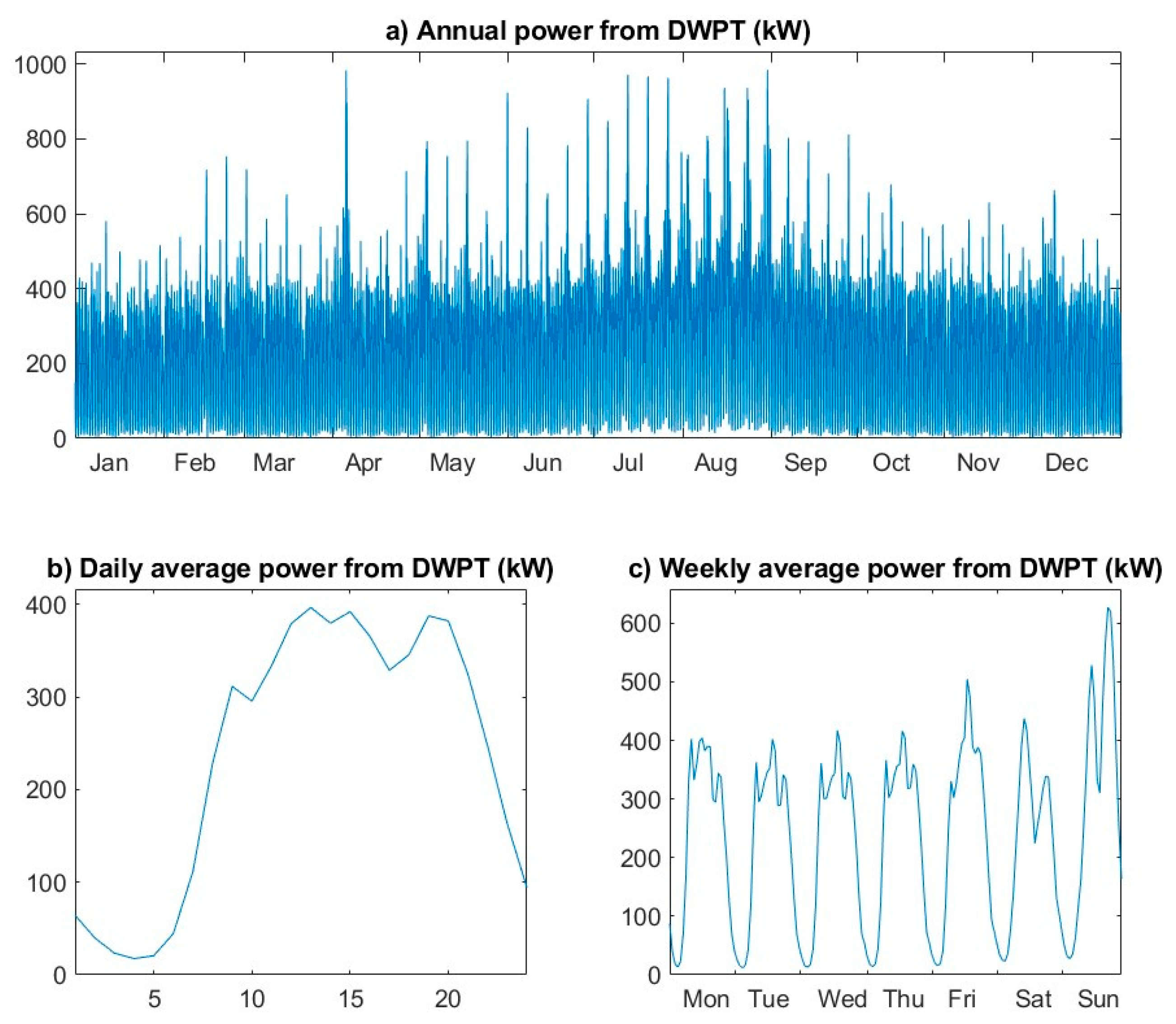
3. Wireless Power Transfer System for the Dynamic Charging of EVs

A DWPT is used to charge EVs traveling on the AP4 Motorway. This road is a 16.2 km-long stretch of motorway between the cities of Puerto Real and Jerez de la Frontera, Spain. The traffic data measured by the two traffic measurement stations (named 85.7C and 85.7D), belonging to the General Directorate of Traffic [46], were used to adequately characterize the traffic on this stretch. Detailed information about the traffic intensity and speed in this stretch of motorway can be found in Reference [10].
The procedure to calculate the electric power demanded by the DWPT system for the EVs charging on this stretch of road was presented in Reference [10]. As in that work, a penetration rate of EVs of 25% with respect to the total number of vehicles has been considered. This penetration value was taken in accordance with the forecasts made by the International Energy Agency in its Global EV Outlook 2016 report [47].
Figure 2 shows the power demanded by the DWPT system for the EVs charging over a year, which was used to size the microgrid. It can be observed that the highest powers are achieved during the summer months, because this stretch of motorway is used a great deal at that time to access to the city of Cadiz.

4. Hydrogen Charging Station for Fuel Cell-Powered Buses

The stand-alone REM also had to supply a hydrogen charging station for FCBs. The hydrogen subsystem, which was composed of an electrolyzer and hydrogen tank, must produce the hydrogen consumed by the FCBs. To size the microgrid, the energy consumption of the hydrogen charging station considering its operating mode was calculated. For this purpose, the demand of inter-city bus lines belonging to the Bahía de Cádiz Transport Consortium was considered [48], with the city of Jerez de la Frontera as the terminus station. Eleven bus lines connect this city with nearby cities. Here, it was assumed that hydrogen buses cover these lines, and they must be recharged from the microgrid, which must provide the energy consumed by the electrolyzer to produce the hydrogen required by the buses for their daily routes. Therefore, the role of the hydrogen subsystem was one of the loads of the hybrid charging station. The microgrid needed to provide the energy consumed by the electrolyzer to produce the hydrogen required by the FCBs for their daily routes. The aim of the optimal sizing of this subsystem was to maintain a minimum hydrogen level in the tank for the whole year, while the system provided the energy required by the vehicles. Additionally, the optimization tried to minimize the volume of the hydrogen tank and the numbers of stackable electrolyzers.
For each route, the kilometers traveled by the bus were estimated, considering the frequencies in weekdays and weekends. The seasons were also considered, since the bus consumption was increased in different ways by the use of heating, ventilating and air conditioning systems. The data and procedures given in Reference [49] were used to make these estimations and subsequent considerations. The average consumption of 12/18-meter-long FCBs was assumed to be 10.0 hydrogen-kg/100 km, which corresponds to the highest value stated in Reference [49]. Furthermore, in January, February, November and December, the consumption of each bus was increased by 2.0 hydrogen-kg/100 km due to the use of heating systems, whereas it was increased by 2.5 hydrogen-kg/100 km in June, July, August and September due to the use of the air conditioning system [49]. The total consumptions obtained for each line were increased by 5% for unforeseen events.
The route named M-560 (between the cities of Jerez de la Frontera and Rota, 31 km long) had the highest consumption in months using the air-conditioner. The daily bus consumption corresponding to this line was 38.8 hydrogen-kg. In all cases, all other lines had lower daily consumption. Following the considerations given in Reference [49], it could be admitted that the fuel-tank of the buses have a capacity of about 50 kg. For this reason, all the buses needed one daily hydrogen charge or refueling.
According to the Society of Automotive Engineers (SAE52601-1), there are three types of hydrogen refueling procedures [49]: (1) slow fueling, with a refueling rate of 1.8 hydrogen-kg/min; (2) normal fueling, with a refueling rate of 3.6 hydrogen-kg/min; and (3) fast fueling, with a refueling rate of up to 7.2 hydrogen-kg/min. In this study, a slow fueling was assumed since the number of buses to be refueled was not high, and the process could be also carried out within a relatively small refueling time window. This had the advantage that the technology used was both simple and cheap.
The required daily hydrogen demand was calculated based on the above. Thus, the maximum value was reached in weekdays during the summer season, with amounts of 257.8 hydrogen-kg per day. Therefore, a slightly higher value of 260 hydrogen-kg was assumed to be the upper consumption limit of the refueling system. This value represents the amount of hydrogen associated with one-day of autonomy in the hydrogen charging station. Since the refueling rate selected was 1.8 hydrogen-kg/min, and the maximum hydrogen demand per day was 260 kg, the charging of all the FCBs could be performed in less than 2.5 h, in the worst case. As a result, a refueling window was set with a start time at 8:00 p.m., when the service on the last line ends. From that moment, the refueling process begins. Depending on the day of the year, the duration may be different, with a maximum duration of 2.5 h as indicated above.
These premises were used to calculate the demand that the proposed microgrid had to satisfy.

5. Optimal Sizing of the Microgrid

As mentioned above, MATLAB-Simulink and SDO were chosen for the optimal sizing of the microgrid under study. Simulink represented the behavior of a dynamic system, while SDO allowed us to apply different types of optimization on the model implemented in Simulink.
The optimization process presented two stages: (1) the definition and implementation of the microgrid model using the Simulink tool, and (2) the sizing optimization of the microgrid using SDO tool.

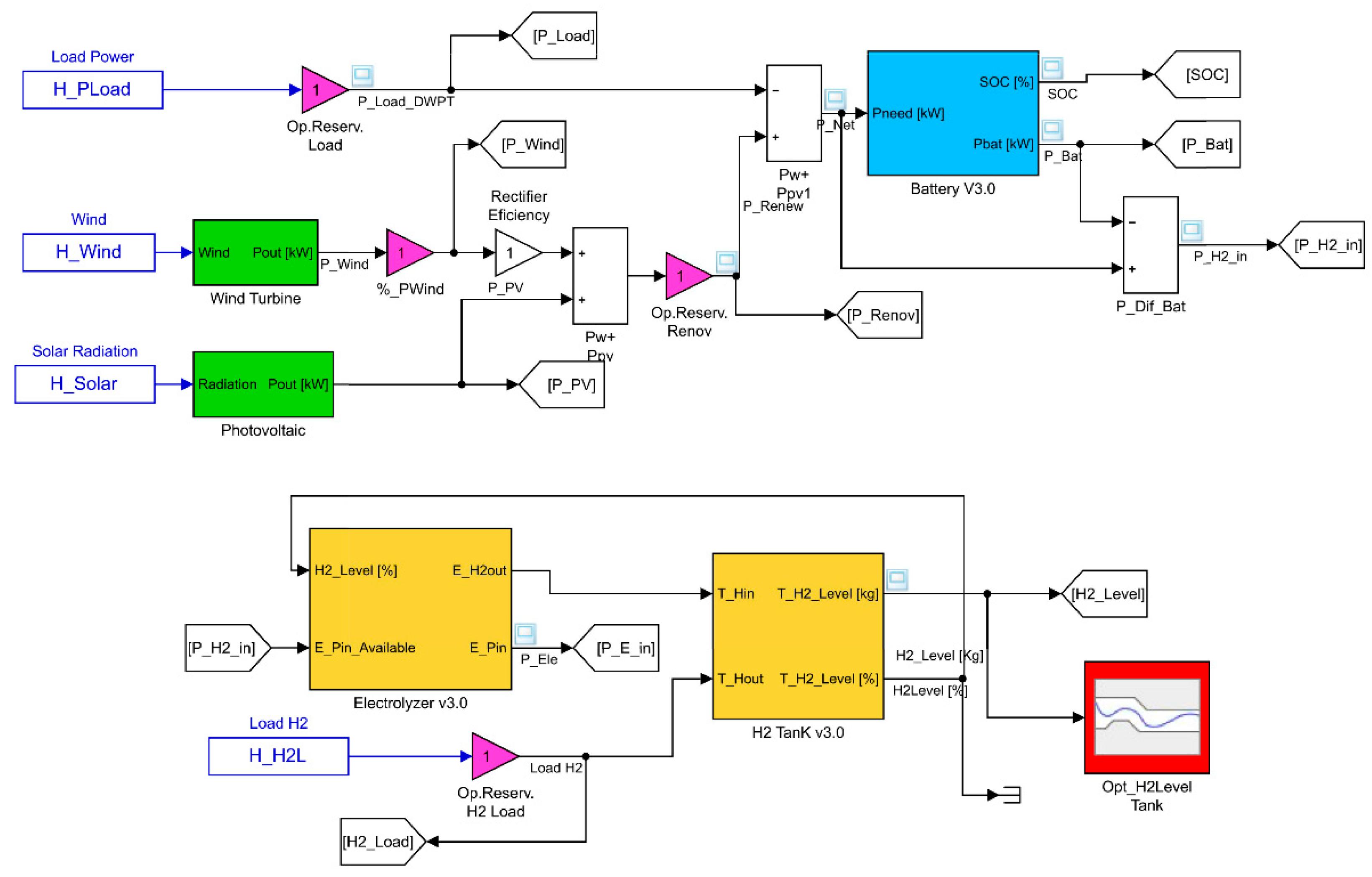
5.1. Simulink Model of the Microgrid

The Simulink model shown in Figure 3 represents the long-term behavior of the microgrid. The system was divided into several subsystems, each of which was represented by a block. The models of each subsystem are described below.

5.1.1. Wind Subsystem

The wind subsystem represents a set of equal WTs, which is represented by the green block named “Wind Turbine”. Here, the sizing parameter was the number of turbines, which was represented by N_W. Initially, calculations were made with three types of turbines: Enercon E44 (rated power, 900 kW); Norwin N200 (200 kW); and Wind Energy Solutions (WES) (70 kW). Due to the specific values of the power requested by the loads, the initial studies carried out with the E44 turbine led to a set of turbines of one unit, or rarely two units. In this case, the range of variability of N_W was very narrow. On the other hand, if WES was used, the number of turbines was always very high, at several tens of turbines. Finally, the N200 turbine was chosen because the resulting number of turbines was around ten.
In this block, the following assumptions were considered: the wind speed incident on each turbine was the same, and the turbines were sufficiently separated one from each other for wake effects not to be considered. The block had one input and one output. A time series of 8760 hourly wind speed values in the selected location, called H_Wind, was used as an input. The statistical data of the wind speed in the place in which the microgrid was planned to be installed were obtained from the information provided by the Andalusian Energy Agency [50]. These data were used to obtain the annual wind time series from the algorithm presented in Reference [51].
As the height at which the wind measurement is made does not usually coincide with the height of the turbine, the time series of wind speed were corrected according to these heights using the following expression:
U t u r b = U m e a s ( z t u r b z m e a s ) ,
where zmeas is the height at which the wind speed is measured; zturb is the height of the turbine; Umeas is the wind speed measured at height zmeas; Uturb is the wind speed at turbine height; and α is the power law exponent, which depends on the rugosity of the terrain.
The output of the WT block provided the electrical output power of the wind subsystem. In order to compute the output power, the power curve profile of the turbine [52] was implemented in this block, using as an input the corrected wind speed time series. Usually, power curves are provided under standard conditions of temperature and pressure. To adjust the output power of the block, the output power given by the power curve was corrected, taking into account the air density in the location, using the following equation:
P W T = P W T S ( ρ ρ 0 )
where PWT is the WT power output; PWTS is the WT power output at standard conditions; ρ is the air density in the location in kg/m3, which only depends on the height of the location above sea level; and ρ0 is the air density at standard conditions (1.225 kg/m3).

5.1.2. Photovoltaic subsystem

The PV subsystem is represented by the green block named “Photovoltaic”. The input of this block was a time series of 8760 hourly incident solar radiation values at the installation site, named H_Solar. This time series was also obtained from the data provided by the Andalusian Energy Agency [53]. The output power of this block is calculated as follows:
P p v = P r · d f G G s t d
where Pr is the rated power of the PV array (kW), df is the derating factor of the PV array (%), G is the solar radiation incident on the PV array (kW/m2), and Gstd is the incident radiation at standard test conditions (i.e., 1 kW/m2). The sizing parameter of the PV subsystem is the rated power of the PV system (P_PV).
The sum of the output powers from the wind subsystem and PV subsystem produced the signal Renewable Power (P_Renew), which represents the power generated by the renewable energy sources of the microgrid. A reduction factor of 0.8 of output power was considered to account for the reduced output in real-world operating conditions compared to the array-rated operating conditions.

5.1.3. Battery Subsystem

The battery subsystem is represented by the light-blue block named “Battery V3.0”. This block had only one input and two outputs. The time series used as an input was the Net Power (P_Net). P_Net is calculated by subtracting the power requested by the EV recharging system from P_Renew (P_Load_DWPT). The output P_Bat provided the power that the battery was capable of storing or producing in the charging and discharging processes, respectively. If this power was positive, the battery was recharged; otherwise, the battery was discharged. The other output was the actual battery state-of-charge (SOC), expressed in a percentage value of the nominal capacity.
In order to calculate the power from the battery system, the KiBam battery model proposed in Reference [54] was implemented. The parameters from Hoppecke OPzS 3000-type batteries [55] were used in this work. Each elemental cell had a nominal voltage of 2 V and a nominal capacity of 3000 Ah. The battery system was composed of a number of strings connected in parallel. In this model, each string had 24 battery cells. Therefore, the nominal capacity of each string was 144 kWh. The sizing parameter of the battery was N_String, which was the number of parallel strings in the subsystem.
The model allowed us to control the battery depending on the SOC of the battery in order to achieve a longer battery life. If the battery SOC equaled, or passed below, the minimum value of 30%, the battery was only allowed to charge. When the battery received enough energy to raise the minimum SOC value, it was allowed to discharge again. If the battery SOC equaled the maximum value of 100%, the battery aws only allowed to discharge. Therefore, the battery system could be used to store/provide energy depending on its actual SOC. For these reasons, the absolute value of output power P_Bat was always less than or equal to the absolute value of the input power P_Net.

5.1.4. Hydrogen Subsystem

The hydrogen subsystem is represented in the Simulink model by two yellow blocks. One of the blocks is called “Electrolyzer v3.0”—modelling the electrolyzer system—and the other block, named “H2 Tank v3.0”, models the behavior of the hydrogen tank.
The Electrolyzer block had two inputs and two outputs. P_H2_in was the difference between P_Net and P_Bat. This difference represented the power that the battery could not manage in the charging/discharging processes. Inside the electrolyzer block, only the positive values of this input could be considered. This meant that it only allowed for the excess power values in the charging process of the battery. Therefore, the block computed the hydrogen production of the electrolyzer subsystem. To do this, the block used the parameters of HyStat hydrogen generators [56]. The Simulink model of the electrolyzer took into account its efficiency. This electrolyzer had a nominal hydrogen flow of 10 Nm3/h and a power consumption of 5.4 kWh/Nm3. Considering the higher heating value of hydrogen as 3.498 kWh/Nm3, the efficiency was 64.77%. This system was stackable, therefore the block considered a stackable number of units of 54 kW each. Thus, the sizing parameter was the number of stackable units, NELE. This block had another input called H2_Level (%). It was necessary to stop hydrogen production when the tank was full. Additionally, the block had two outputs. E_Pin represents the electrical energy used by the electrolyzer in the hydrogen production; because not all the electrical energy was always available in the input, E_Pin_Available was used in the hydrogen production. The other output was E_H2out, which provided the current value of hydrogen production in kilograms.
The last block of the subsystem was the hydrogen tank block. In this case, the sizing parameter of this block was NTank, which represented the number of stackable units of 10 kg each. This block had two outputs: the current hydrogen levels in the tank expressed in kilograms (T_H2_Level (kg) output) and as percentage of the maximum capacity (T_H2_Level (%) output). The block also had two inputs: the mass of incoming hydrogen in the tank (T_Hin = E_H2out), and the hydrogen demand (T_Hout = H_H2L), which was obtained from a time series of 8760 values with the hourly hydrogen needs of the refueling system described in Section 4.

5.2. Sizing Optimization Based on SDO

SDO was the MATLAB-Simulink tool used in this paper for the optimal sizing of the microgrid. SDO allowed us to perform various types of optimization with different strategies. It had the main advantage that it was very easy to implement the algorithm.
SDO offers tools for analyzing and tuning parameters in Simulink models. Several types of analysis can be carried out. One of them is “Response Optimization”, which allowed us to size the parameters of a system in order to maintain them between two established limits or to follow a reference signal. When SDO carries out a Response Optimization, it converts the requirements of the Simulink model into a constrained optimization problem. Then, the problem is solved by using optimization algorithms. SDO simulates the Simulink model iteratively by assigning values to the parameters. After each simulation, SDO compares the results with the constraints, and then uses optimization methods to modify the parameters in order to meet the objectives. SDO can formulate three types of minimization problems: a feasibility problem, a tracking problem or a mixed feasibility and tracking problem. In the first case, the optimization algorithm tries to find the parameter values that satisfy all constraints within the specified tolerances. In tracking problems, a reference signal is specified, and the sum-squared error tracking is minimized. Mixed problems use both strategies.
In this paper, the objective of the optimization was to select the sizing parameters to be able to cover both the power demand of the DWPT system for the EV charging and the power demand of the electrolyzer in order to meet the hydrogen demand of the bus refueling system. The hydrogen tank level was an output variable, and the main goal was to maintain an adequate stored hydrogen level. This level, which was variable throughout the year, had to be maintained between two values: the maximum corresponding to the tank capacity, and the minimum corresponding to the level of hydrogen associated to the desired autonomy.
For all the above, the most appropriate minimization problem was the feasibility problem. In this case, at least a constraint signal had to be specified (hydrogen tank level) and a check block was added to this signal in the Simulink model. In this block, piecewise linear lower and upper bounds were defined. For each iteration, the software computed the distance between the simulated response and the bounds. If all the constraints defined were met for some combination of the parameter values, then that solution was considered valid.
Three types of methods are available: the Gradient Descend Method, which uses the optimization function fmincon from the Optimization Toolbox; the Simplex Search Method, which uses the functions fminsearch and fminbnd from the Optimization Toolbox; and the Pattern Search Method, which uses the function patternsearch from the Global Optimization Toolbox. To solve the problem, all three methods were tested. Only the Pattern Search method allowed us to always converge on the results, and so it became the method used in all analyzes. In feasibility problems, the Pattern Search Method formulates the constraint and then minimizes the maximum constraint violation. More information regarding these optimization functions can be found in Reference [57]. The tolerance value used in the method was 1 × 10⁻⁵. This value was obtained by successive executions looking for a compromise solution between runtime and accuracy.
An optimization process with SDO involves several steps:
(1)
Model construction and definition of the design variables (DVs). The DVs are the parameters involved in the optimization process; in this case, the sizing parameters of the subsystems. The signals that are subject to restrictions in the Response Optimization analysis must be also defined. In this case, an annual minimum constraint to the hydrogen level in the tank was established. This constraint was carried out through the red block, called “Opt_H2Level Tank” in Figure 3. Different minimum hydrogen levels were analyzed in this work, but in all cases, the minimum levels were integers of the daily hydrogen maximum demand established in 260 hydrogen-kg per day in Section 4.
(2)
Definition of the range of variation and the starting value of the DVs to be used in the optimization process. The range of values (maximum and minimum) and the initial values of the DVs must be defined. The detailed procedure followed to define these ranges of values is not indicated here due to the length of the paper, and only the criteria followed to select the limits of those ranges are briefly stated. The maximum number of WTs, as well as the maximum value of the installed PV power, are defined by the average capacity of joint energy production with respect to the average energy requested by the load for the most unfavorable month. The obtained values were 16 units for N_WT_max and 3152 kW for P_PV_max. The maximum number of strings in the subsystem battery was calculated for the day of the year with the greatest energy requested by the load. This energy was considered 70% of the maximum energy of the battery. This led to 176 strings. The maximum number of stackable units of the electrolyzer was chosen considering that its capacity of hydrogen production was equal to the maximum daily demand of hydrogen by the refueling station. The value obtained was 121 units. The maximum value of the last DV and the number of stackable hydrogen tank units was taken as equal to a sufficiently large arbitrary value. For this model, the assigned value was 1000 units.

6. Results and Discussions

The optimization process presented in this study was applied in two phases. First, only the sizing of the hydrogen subsystem was optimized. This partial optimization allowed us to compare the results from SDO with those obtained directly from the model, in order to contrast the results achieved. Later, the sizing of the whole system was optimized.

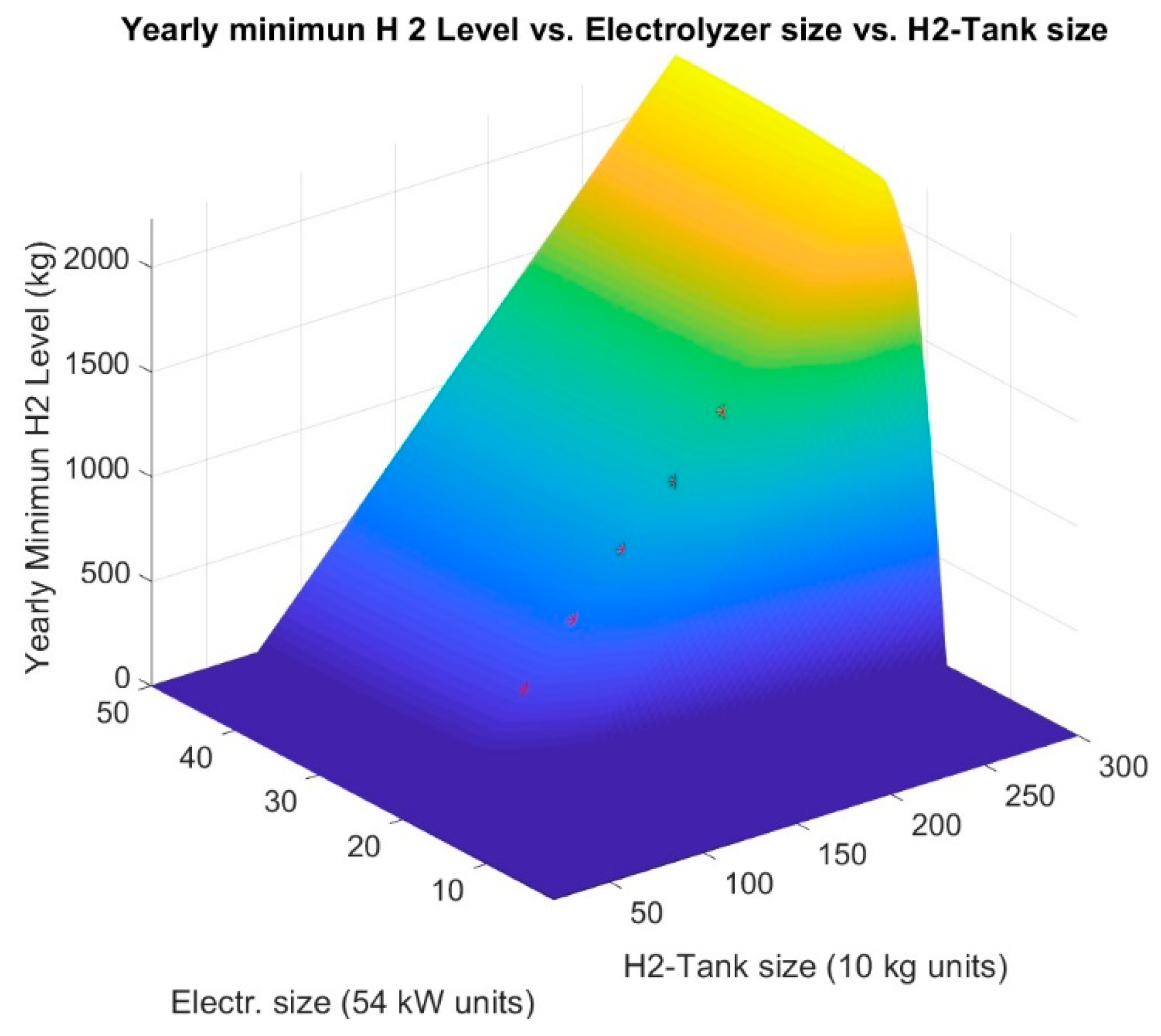
6.1. SDO-Based Sizing Optimization of the Hydrogen Subsystem

In this case, only the hydrogen subsystem was optimized. Thus, the sizing parameters of other subsystems were unaffected. These parameters were N_W, P_PV and N_String. In order to perform the optimization, the values of these parameters were defined close to their optimum values. As the optimization of the whole system had not yet been carried out, a partial pre-sizing was carried out for these subsystems. The sizing values obtained were 10 units for N_W, 2366 kW for P_PV, and 44 strings for N_String.

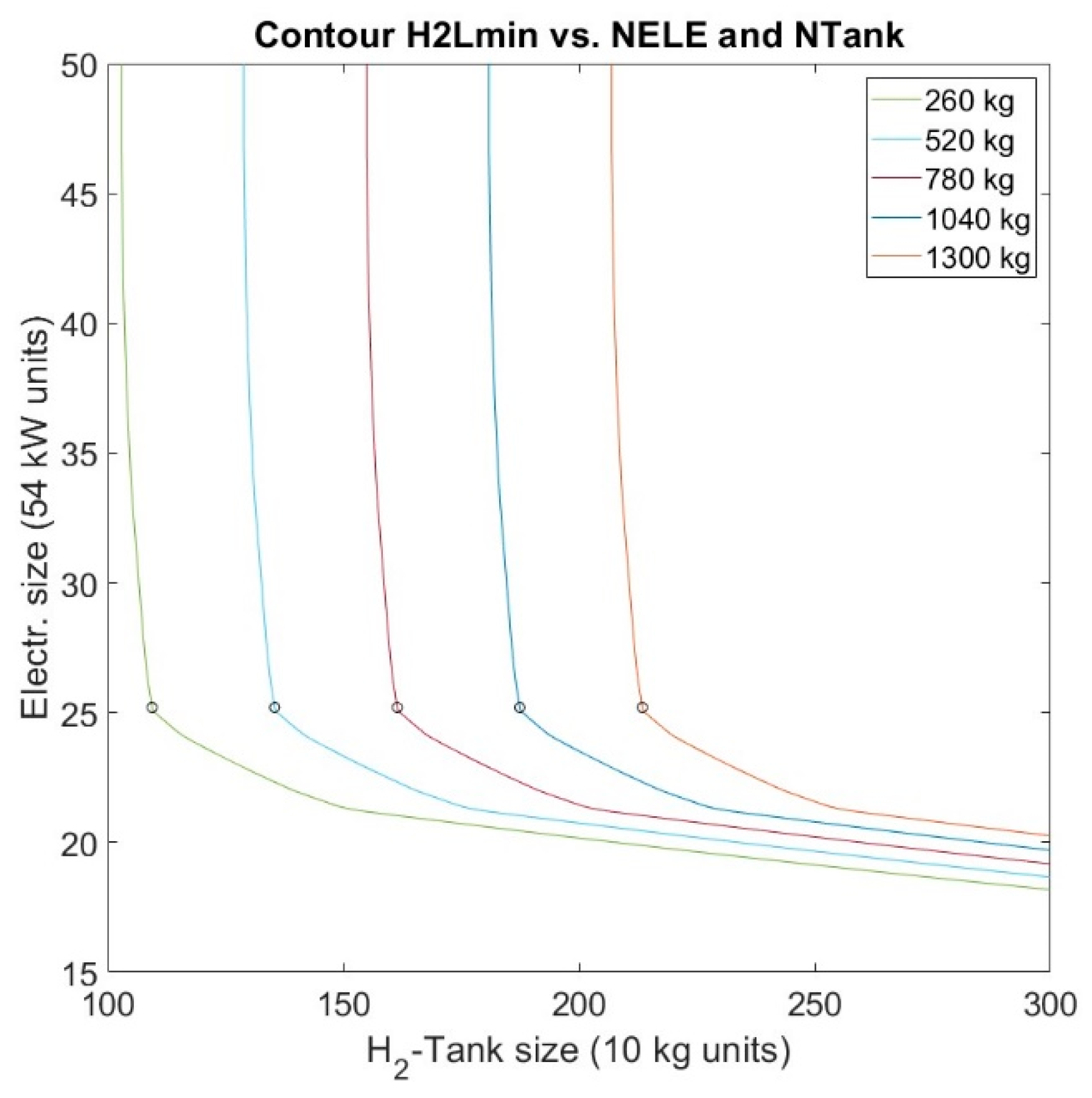
6.1.1. Dependence on the Minimum Level of Hydrogen

Before optimizing with SDO, a study was made with the Simulink model to consider the dependence of the annual minimum hydrogen level (H2Lmin) in the tank with NELE and NTank. The results from this analysis were compared with those obtained with SDO, in order to verify the results of the optimization procedure proposed here. The Simulink system model was executed for one year. The values of the sizing parameters N_W, P_PV and N_String were fixed to those indicated above, while NTank and NELE were varied, in steps of 0.1 units, between the minimum and maximum values obtained by the SDO analysis performed in the previous section.
Figure 4 depicts the results obtained from the analysis. The dependence of H2Lmin on NELE and NTank can be observed. If NTank values were lower than 79.5 units, the values of H2Lmin were always zero for any value of NELE. Likewise, if NELE values were lower than 17.5 units, H2Lmin was always zero for any NTank value. On the other hand, for NTank values higher than 79.5 units, the obtained H2Lmin value was almost constant regardless of the NELE value. A similar situation occurred with the H2Lmin value obtained for NELE values higher than 17.5 units, where it remained practically constant. For this reason, the dependency surface was formed by two almost flat surfaces, except for the intersection of both surfaces which presented a certain curvature.

6.1.2. Optimal Sizing of the Hydrogen Subsystem

The aim of the optimal sizing of the hydrogen subsystem was to maintain a minimum hydrogen level in the tank for the whole year, while the system provided the energy required by the DWPT to charge the EVs and to produce the hydrogen consumed by the FCBs, taking advantage of all the energy produced by renewable sources. This minimum value was the same as the maximum daily consumption of the hydrogen charging station; i.e., 260 hydrogen-kg, as indicated in Section 5.2. In this case, the optimized DVs were NTank and NELE. Their maximum value DVs were indicated in Section 5.2, at 121 and 1000 units, respectively. The minimum values were one unit for both parameters. The rest of the sizing parameters were fixed to the values indicated at the beginning of Section 6.1.
As mentioned before, the approach of the optimization problem in SDO may include additional constraints. The following constraints completed the optimization problem definition:
  • Minimization of the H2Lmin value: This constraint forces SDO to minimize the H2Lmin value.
  • Minimization of NTank and NELE: These constraints force SDO to find a solution that minimizes the values of the hydrogen subsystem parameters.
  • The battery SOC was kept above 30%: The battery model has a control over the minimum SOC, but it does not prevent this limit from being reached. The minimization process of the size causes a greater demand of energy to the battery and repeated processes of discharge below the minimum SOC. This constraint was included in order to prevent that situation.
Five studies were performed with SDO for a hydrogen autonomy between one and five days (260 to 1300 hydrogen-kg). The results are shown in Table 1. This table also shows the final values of NELE and NTank parameters, the minimum annual value of the hydrogen level in the tank (H2Lmin), and the tank level at the end of the year (H2Lend) in kilograms and in percentages. The values of NELE and NTank parameters obtained with SDO are represented by red stars on the surface shown in Figure 4.
Figure 5 shows the annual evolution of the battery SOC (%), the power requested by the electrolyzer (kW), and the hydrogen tank level during a whole year, for the sizing in the case of one day of autonomy. The minimum hydrogen tank level, 260 kg, was only reached in mid-August. The battery SOC was maintained above 30% throughout the year in order to preserve its lifetime. The minimum SOC value was 41.1% at the end of July.

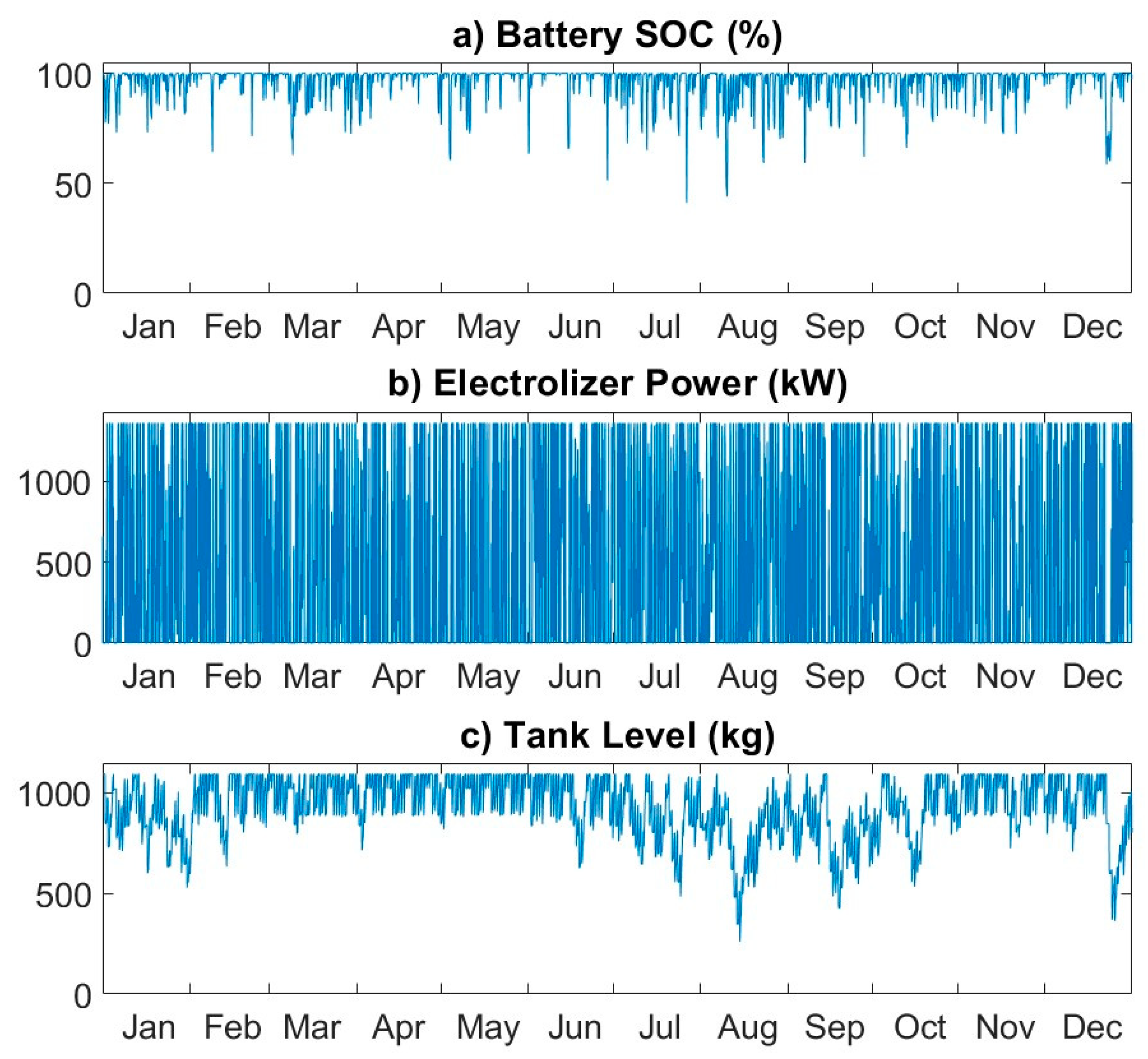
6.1.3. Checking the Results Obtained by SDO

The study carried out with the Simulink system model in Section 6.1.1 was used to validate the results obtained by SDO. The minimum annual values of H2Lmin obtained by varying the sizing parameters of hydrogen subsystem in a wide range of values were compared with the optimal sizing with SDO.
If the surface of dependence of H2Lmin with NELE and NTank, shown in Figure 4, is intersected with a horizontal plane at a given height by the annual minimum level H2Lmin considered, the result is a line. This line represents all the pairs of values (NELE, NTank) that allow us to achieve the given H2Lmin value. If the minimum value of both parameters in this line is computed, the minimum values of the sizing parameters of the hydrogen subsystem for the H2Lmin considered are obtained. Performing these operations with each of the H2Lmin levels considered in Section 6.1.2, the curved lines of pairs of values (NELE, Ntank), shown in Figure 6, are achieved. In the same figure, the location of the minimum value of NELE and NTank is represented with a circle on each line.
Table 2 shows the numerical values obtained for the NELE and NTank parameters by using this procedure. In addition, for each parameter, the relative error of the result obtained by SDO is indicated. As can be seen, the error obtained in all cases by SDO was less than 0.8%.
In conclusion, the sizing obtained by the proposed SDO procedure provided correct results. In addition, the procedure proposed in this article offers the advantage of being much faster than obtaining the values by using the model and varying the sizing parameters in the range of values set. The execution times depend on many factors such as the number of sizing parameters, system configuration and type of computer used. In this case, the execution time to obtain the response of the model by varying the parameters was 24 times greater than the execution time of the proposed sizing procedure with SDO, even though the step considered in the parameter variation with the model was 0.1 units and the tolerance set of the parameters used in SDO was much more restrictive (1 × 10⁻⁵).

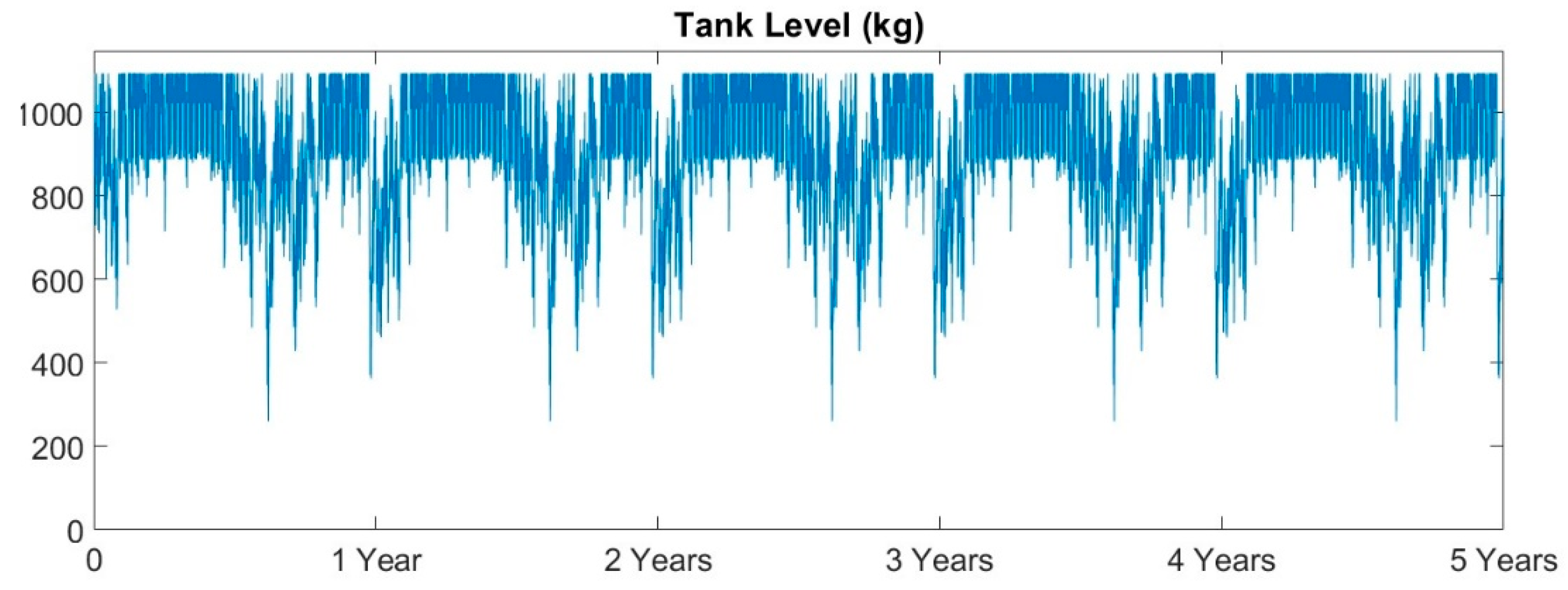
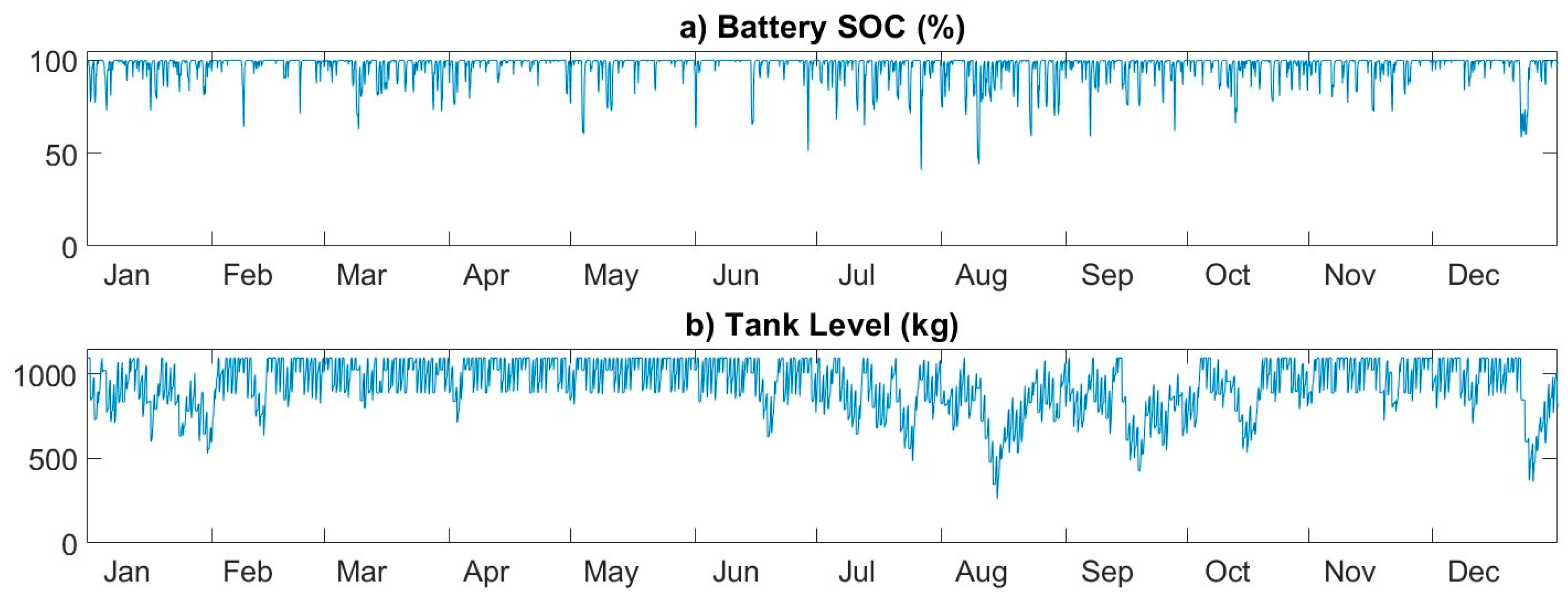
6.1.4. Annual Final Value of the Hydrogen Tank Level

All the SDO calculations presented in the previous sections were performed considering an initial hydrogen tank level of 100%. As can be observed, in all cases, the final level was lower. This may give the idea that a gradual decrease in the hydrogen tank level will occur in successive years; however, this does not have to be the case, since the final value of the hydrogen tank level will depend not only on the initial level but also on renewable energy production during the year.
To verify this, a system simulation was carried out for five years by using the sizing parameters obtained for a minimum hydrogen autonomy of one day. The hydrogen tank level during this time is shown in Figure 7. Although the level at the end of the first year was not 100%, the final level of the hydrogen tank at the end of successive years was not affected. In any case, this is a particular feature of the system under study. Obviously, this could not happen in other cases. If so, SDO is flexible enough to deal with this problem. For example, the problem could be easily reformulated in SDO to achieve the optimal sizing of the microgrid, if the final level of the hydrogen tank must be similar to the initial level. To implement this, it would be enough to add two additional restrictions to SDO to those already used: one for the initial level of the hydrogen tank, for which its minimization would be requested, and another restriction that minimizes the difference between the final and initial level of the hydrogen tank.
For a minimum hydrogen autonomy of one day and a difference between the final and the initial level of the hydrogen tank of 1%, the sizing results obtained by SDO were the following:
  • NELE: 17.6 units of 54 kW.
  • NTank: 331.9 units of 10 kg.
  • Minimum initial level of the hydrogen tank: 79.5%.
  • Final annual level of the hydrogen tank: 80.3%, or 2664 kg.

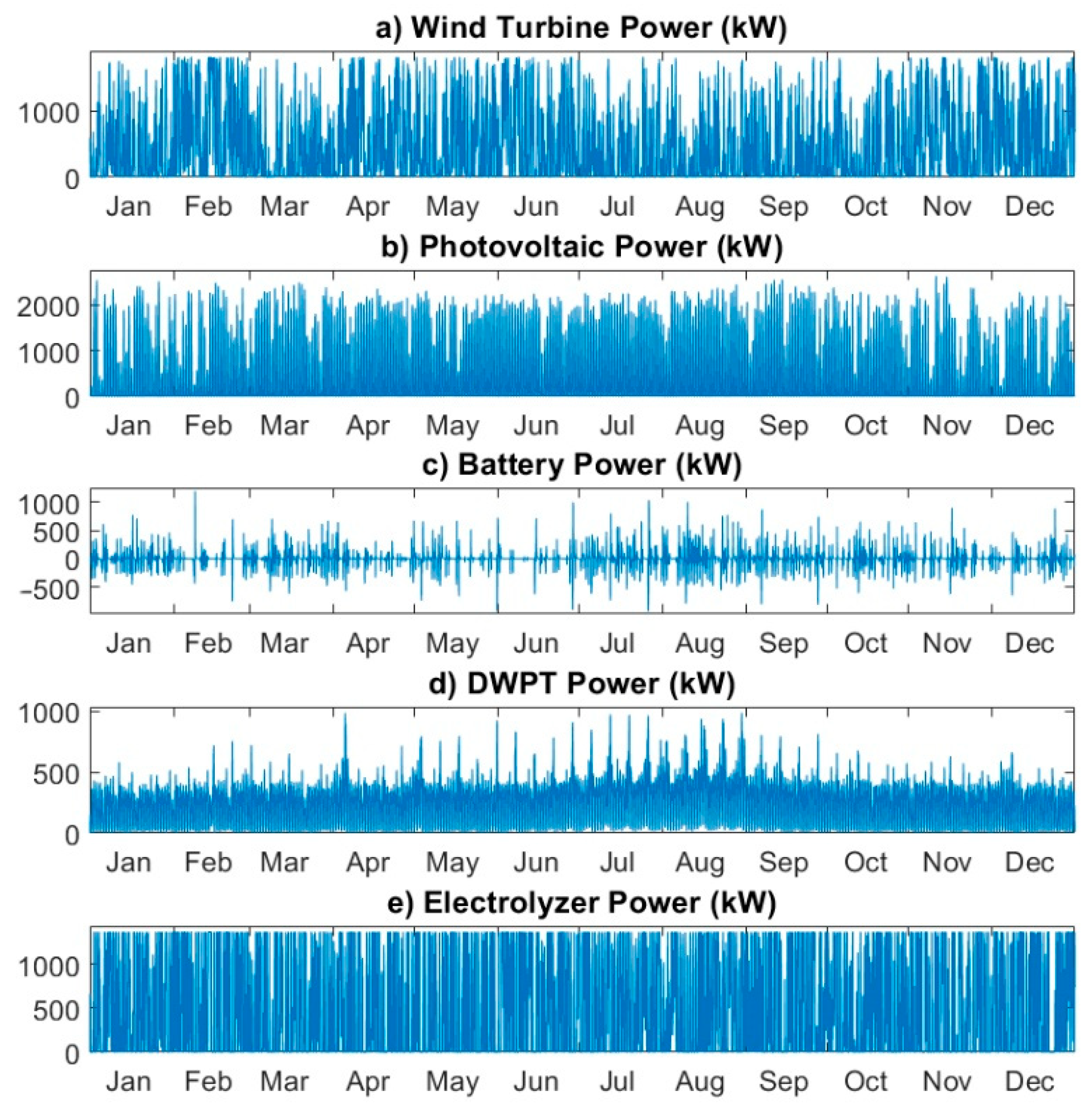
6.2. SDO-Based Optimal Sizing of the Whole Microgrid

Once it was verified that the optimal sizing procedure of the hydrogen subsystem with SDO gave correct results, the same procedure was applied for the optimal sizing of the complete microgrid. For this task, the DVs used in SDO were the five sizing parameters of the microgrid: N_W, P_PV, N_String, NTank and NELE. For all these variables, the constraints were defined in order to minimize them. The minimum and maximum values considered in the DVs variables were determined by the procedure proposed in Section 5.2. Again, the restrictions were to minimize H2Lmin and to keep the SOC of the battery subsystem above 30%. The sizing obtained for a minimum hydrogen autonomy of a day is shown in Table 3.
In this case, Figure 8 shows the annual evolution of the different powers involved in the microgrid. The power from renewable sources are shown in Figure 8a,b. It can be observed that the power production from the WTs had a stochastic evolution, while the power production from the PV panels was greater during the spring and summer than in the other two seasons. Figure 8c shows the power managed by the battery subsystem. The positive values corresponded to the power handled by the battery in the charge process, while the negative values corresponded to the power handled in the discharge. During the whole year, the use of the battery was almost continuous and balanced. In February and June, the battery was used less, because the total renewable production was higher. On the other hand, during the months of July, August and September, the use of the battery subsystem was greater due to the increase in the power demand requested by the DWPT system. The power requested by the DWPT system is illustrated in Figure 8d. Finally, Figure 8e depicts the power requested by the electrolyzer. This power was greater than the power requested by the DWPT system and was fairly constant throughout the year.
Figure 9 illustrates the annual evolution of the battery SOC and the hydrogen tank level. With the optimal sizing achieved with SDO, the minimum hydrogen tank level was also reached in mid-August. In this case, the hydrogen tank level was lower during the winter months. The battery SOC achieved the minimum value of 30% on mid-July. As can be seen in this figure, the use of battery power is somewhat more intense in summer.

7. Conclusions

This paper presented a new, long-term optimal sizing and evaluation method of a stand-alone microgrid, comprising renewable energy sources (WT and PV) and a battery as energy storage, for the dynamic wireless charging of EVs and a hydrogen charging station for FCBs.
First, the procedures followed to define the electrical demand for both the charging systems of EVs and FCBs were presented. Second, the models of the different subsystems were introduced. Then, the tools proposed to carry out the optimal sizing based on SDO were presented. Simulink was used to create a dynamic model of the microgrid. SDO was used to optimize the parameter sizing of the model in order to achieve an adequate performance of the system according to the fixed constraints. Initially, the optimal sizing of the hydrogen subsystem was carried out with SDO to keep an annual minimum level of the hydrogen tank and thus the autonomy of the charging system of the FCBs. The results obtained with SDO for the optimal hydrogen subsystem were compared with those obtained by the execution of the model of the microgrid in all possible cases, and thus it was proved that SDO offered the optimal results.
The optimal sizing was applied to the complete microgrid. The results showed that the designed system was able to provide the energy requested by the DWPT for charging the EVs, and that needed to produce the hydrogen consumed by the FCBs, taking advantage of all the energy produced by renewable sources, considering a certain autonomy (or reserve) in the hydrogen subsystem and avoiding the excess discharge of the battery in order to extend its useful life.
Finally, it is worth noting that the methodology presented in this work based on SDO presents the following advantages: (1) the model and control strategy of the microgrid and the optimization algorithm can be easily implemented; (2) it can be used by users without deep optimization knowledge; (3) it allows the implementation of mono- and multi-objective optimization; and (4) it offers great flexibility, since it could be used for analyzing other possible scenarios and design requirements and aids in the design and evaluation of other types of configurations or microgrids. The main limitation of this methodology is that SDO has limited the optimization algorithms to be used, but that allows us to solve and find the optimal solution for a wide range of optimization problems (linear and nonlinear).

Author Contributions

Conceptualization, methodology and investigation, H.S.-S., C.-A.G.-V., F.L.I. and L.M.F.-R.; software and validation, H.S.-S.; writing and supervision, H.S.-S., C.-A.G.-V., F.L.I. and L.M.F.-R.; project administration, L.M.F.-R.

Funding

This work was partially funded by the Spanish Ministry of Economy and Competitiveness under Grant ENE2013-46205-C5- 1-R.

Acknowledgments

We thank the Spanish Directorate-General for Traffic (“Dirección General de Tráfico, DGT”) for providing the traffic data.

Conflicts of Interest

The authors declare no conflict of interest.

References

  1. European Commission. State of the Art on Alternative Fuels Transport Systems in the European Union; European Commission: Brussel, Belgium, 2015. [Google Scholar]
  2. Energy-Economics-Environment Modeling Laboratory. Available online: http://www.e3mlab.eu/e3mlab/index.php (accessed on 27 October 2018).
  3. 2014-PRIMES-TREMOVE: A Transport Sector Model for Long-Term Energy-Economy-Environment Planning for EU. Available online: http://www.e3mlab.eu/e3mlab/index.php?option=com_content&view=article&id=485%3A2014-qprimes-tremove-a-transport-sector-model-for-long-term-energy-economy-environment-planning-for-euq&catid=54%3Apresentations&Itemid=79&lang=en (accessed on 27 October 2018).
  4. Li, S.; Mi, C.C. Wireless power transfer for electric vehicle applications. IEEE J. Emerg. Sel. Top. Power Electron. 2015, 3, 4–17. [Google Scholar]
  5. Vilathgamuwa, D.M.; Sampath, J.P.K. Wireless power transfer (WPT) for electric vehicles (EVs)—Present and future trends. In Plug in Electric Vehicles in Smart Grids; Springer: Singapore, 2015; Volume 91, pp. 33–60. ISBN 978-981-287-301-9. [Google Scholar]
  6. Ko, Y.D.; Jang, Y.J. The optimal system design of the online electric vehicle utilizing wireless power transmission technology. IEEE Trans. Intell. Transp. Syst. 2013, 14, 1255–1265. [Google Scholar] [CrossRef]
  7. Jeong, S.; Jang, Y.J.; Kum, D. Economic Analysis of the Dynamic Charging Electric Vehicle. IEEE Trans. Power Electron. 2015, 30, 6368–6377. [Google Scholar] [CrossRef]
  8. Miller, J.M.; Jones, P.T.; Li, J.M.; Onar, O.C. ORNL experience and challenges facing dynamic wireless power charging of EV’s. IEEE Circuits Syst. Mag. 2015, 15, 40–53. [Google Scholar] [CrossRef]
  9. Transport Research Laboratory (TRL). Feasibility Study: Powering Electric Vehicles on England’s Major Roads; Highways England Company: London, UK, 2015; Volume 244. [Google Scholar]
  10. García-Vázquez, C.A.; Llorens-Iborra, F.; Fernández-Ramírez, L.M.; Sánchez-Sainz, H.; Jurado, F. Comparative study of dynamic wireless charging of electric vehicles in motorway, highway and urban stretches. Energy 2017, 137, 42–57. [Google Scholar] [CrossRef]
  11. Fabric-Fabric EU Project. Available online: https://www.fabric-project.eu/ (accessed on 28 October 2018).
  12. De Silva, R.; Fisk, K. Charging electric vehicles from distributed solar generation. In Proceedings of the 2015 IEEE PES Asia-Pacific Power and Energy Engineering Conference (APPEEC), Brisbane, Australia, 15–18 November 2015; pp. 1–5. [Google Scholar]
  13. Chandra Mouli, G.R. Charging Electric Vehicles from Solar Energy: Power Converter, Charging Algorithm and System Design. Doctoral Dissertation, Delft University of Technology, Hong Kong, China, 2018. [Google Scholar]
  14. Correa, G.; Muñoz, P.; Falaguerra, T.; Rodriguez, C.R. Performance comparison of conventional, hybrid, hydrogen and electric urban buses using well to wheel analysis. Energy 2017, 141, 537–549. [Google Scholar] [CrossRef]
  15. Kendall, K.; Kendall, M.; Liang, B.; Liu, Z. Hydrogen vehicles in China: Replacing the Western Model. Int. J. Hydrog. Energy 2017, 42, 30179–30185. [Google Scholar] [CrossRef]
  16. Lozanovski, A.; Whitehouse, N.; Ko, N.; Whitehouse, S. Sustainability assessment of fuel cell buses in public transport. Sustainability 2018, 10, 1480. [Google Scholar] [CrossRef]
  17. Barboza, C. Towards a renewable energy decision making model. Procedia Comput. Sci. 2015, 44, 568–577. [Google Scholar] [CrossRef]
  18. NewBusFuel. Available online: http://newbusfuel.eu/ (accessed on 28 October 2018).
  19. Edwards, R.; Hass, H.; Larivé, J.-F.; Lonza, L.; Mass, H.; Rickeard, D.; Larive, J.-F.; Rickeard, D.; Weindorf, W. Well-to-Wheels Analysis of Future Automotive Fuels and Powertrains in the European Context WELL-TO-TANK (WTT) Report; Version 4; U.S. Department of Energy: Washington, DC, USA, 2013.
  20. Al-falahi, M.D.A.; Jayasinghe, S.D.G.; Enshaei, H. A review on recent size optimization methodologies for standalone solar and wind hybrid renewable energy system. Energy Convers. Manag. 2017, 143, 252–274. [Google Scholar] [CrossRef]
  21. Amutha, W.M.; Rajini, V. Techno-economic evaluation of various hybrid power systems for rural telecom. Renew. Sustain. Energy Rev. 2015, 43, 553–561. [Google Scholar] [CrossRef]
  22. Bentouba, S.; Bourouis, M. Feasibility study of a wind–photovoltaic hybrid power generation system for a remote area in the extreme south of Algeria. Appl. Therm. Eng. 2016, 99, 713–719. [Google Scholar] [CrossRef]
  23. Akram, U.; Khalid, M.; Shafiq, S. An Improved Optimal Sizing Methodology for Future Autonomous Residential Smart Power Systems. IEEE Access 2018, 6, 5986–6000. [Google Scholar] [CrossRef]
  24. Zhao, B.; Zhang, X.; Li, P.; Wang, K.; Xue, M.; Wang, C. Optimal sizing, operating strategy and operational experience of a stand-alone microgrid on Dongfushan Island. Appl. Energy 2014, 113, 1656–1666. [Google Scholar] [CrossRef]
  25. Bartolucci, L.; Cordiner, S.; Mulone, V.; Rocco, V.; Rossi, J.L. Hybrid renewable energy systems for renewable integration in microgrids: Influence of sizing on performance. Energy 2018, 152, 744–758. [Google Scholar] [CrossRef]
  26. Nogueira, C.E.C.; Vidotto, M.L.; Niedzialkoski, R.K.; De Souza, S.N.M.; Chaves, L.I.; Edwiges, T.; Dos Santos, D.B.; Werncke, I. Sizing and simulation of a photovoltaic-wind energy system using batteries, applied for a small rural property located in the south of Brazil. Renew. Sustain. Energy Rev. 2014, 29, 151–157. [Google Scholar] [CrossRef]
  27. Ferrer-Martí, L.; Domenech, B.; García-Villoria, A.; Pastor, R. A MILP model to design hybrid wind-photovoltaic isolated rural electrification projects in developing countries. Eur. J. Oper. Res. 2013, 226, 293–300. [Google Scholar] [CrossRef]
  28. Kanase-Patil, A.B.; Saini, R.P.; Sharma, M.P. Sizing of integrated renewable energy system based on load profiles and reliability index for the state of Uttarakhand in India. Renew. Energy 2011, 36, 2809–2821. [Google Scholar] [CrossRef]
  29. Rajanna, S.; Saini, R.P. Development of optimal integrated renewable energy model with battery storage for a remote Indian area. Energy 2016, 111, 803–817. [Google Scholar] [CrossRef]
  30. Fathy, A. A reliable methodology based on mine blast optimization algorithm for optimal sizing of hybrid PV-wind-FC system for remote area in Egypt. Renew. Energy 2016, 95, 367–380. [Google Scholar] [CrossRef]
  31. Sanchez, V.M.; Chavez-Ramirez, A.U.; Duron-Torres, S.M.; Hernandez, J.; Arriaga, L.G.; Ramirez, J.M. Techno-economical optimization based on swarm intelligence algorithm for a stand-alone wind-photovoltaic-hydrogen power system at south-east region of Mexico. Int. J. Hydrog. Energy 2014, 39, 16646–16655. [Google Scholar] [CrossRef]
  32. Shi, B.; Wu, W.; Yan, L. Size optimization of stand-alone PV/wind/diesel hybrid power generation systems. J. Taiwan Inst. Chem. Eng. 2017, 73, 93–101. [Google Scholar] [CrossRef]
  33. Singh, S.; Singh, M.; Kaushik, S.C. Feasibility study of an islanded microgrid in rural area consisting of PV, wind, biomass and battery energy storage system. Energy Convers. Manag. 2016, 128, 178–190. [Google Scholar] [CrossRef]
  34. Ahmadi, S.; Abdi, S. Application of the Hybrid Big Bang-Big Crunch algorithm for optimal sizing of a stand-alone hybrid PV/wind/battery system. Sol. Energy 2016, 134, 366–374. [Google Scholar] [CrossRef]
  35. Cho, J.H.; Chun, M.G.; Hong, W.P. Structure optimization of stand-alone renewable power systems based on multi object function. Energies 2016, 9, 649. [Google Scholar] [CrossRef]
  36. Mukhtaruddin, R.N.S.R.; Rahman, H.A.; Hassan, M.Y.; Jamian, J.J. Optimal hybrid renewable energy design in autonomous system using Iterative-Pareto-Fuzzy technique. Int. J. Electr. Power Energy Syst. 2015, 64, 242–249. [Google Scholar] [CrossRef]
  37. HOMER (The Hybrid Optimization Model for Electric Renewables). Available online: http://homerenergy.com/ (accessed on 30 September 2019).
  38. HOGA (Hybrid Optimization by Genetic Algorithms). Available online: https://ihoga.unizar.es/en/ (accessed on 30 September 2019).
  39. Zahboune, H.; Zouggar, S.; Krajacic, G.; Varbanov, P.S.; Elhafyani, M.; Ziani, E. Optimal hybrid renewable energy design in autonomous system using Modified Electric System Cascade Analysis and Homer software. Energy Convers. Manag. 2016, 126, 909–922. [Google Scholar] [CrossRef]
  40. Han, Y.; Zhang, G.; Li, Q.; You, Z.; Chen, W. Hierarchical energy management for PV/hydrogen/battery island DC microgrid. Int. J. Hydrog. Energy 2019, 44, 5507–5516. [Google Scholar] [CrossRef]
  41. Simulink Design Optimization Product Description-MATLAB & Simulink. Available online: https://www.mathworks.com/products/sl-design-optimization.html (accessed on 31 October 2018).
  42. Simulink-Simulation and Model-Based Design-MATLAB & Simulink. Available online: https://www.mathworks.com/products/simulink.html (accessed on 2 October 2018).
  43. Castañeda, M.; Cano, A.; Jurado, F.; Sánchez, H.; Fernández, L.M. Sizing optimization, dynamic modeling and energy management strategies of a stand-alone PV/hydrogen/battery-based hybrid system. Int. J. Hydrog. Energy 2013, 38, 3830–3845. [Google Scholar] [CrossRef]
  44. Cano, A.; Jurado, F.; Sánchez, H.; Fernández, L.M.; Castañeda, M. Optimal sizing of stand-alone hybrid systems based on PV/WT/FC by using several methodologies. J. Energy Inst. 2014, 87, 330–340. [Google Scholar] [CrossRef]
  45. Lata-García, J.; Reyes-Lopez, C.; Jurado, F.; Fernández-Ramírez, L.M.; Sanchez, H. Sizing optimization of a small hydro/photovoltaic hybrid system for electricity generation in Santay Island, Ecuador by two methods. In Proceedings of the 2017 CHILEAN Conference on Electrical, Electronics Engineering, Information and Communication Technologies (CHILECON), Pucon, Chile, 18–20 October 2017. [Google Scholar]
  46. Ministerio del Interior de España Dirección General de Tráfico. Available online: www.dgt.es (accessed on 11 October 2018).
  47. International Energy Agency. Global EV Outlook 2016; Int. Energy Agency: Paris, France, 2016. [Google Scholar]
  48. Consorcio de Transportes Bahía de Cádiz. Available online: http://www.cmtbc.es/ (accessed on 11 October 2018).
  49. FCH. New Bus Refuelling for European Hydrogen Bus Depots; CORDIS, European Commission: Luxemburg, 2016. [Google Scholar]
  50. AAE-Agencia Andaluza de la Energía Agencia Andaluza de la Energía. Mapa Eólico. Available online: https://www.agenciaandaluzadelaenergia.es/MapaEolico/index.jsp (accessed on 16 October 2018).
  51. Aksoy, H.; Toprak, Z.F.; Aytek, A.; Unal, N.E. Stochastic generation of hourly mean wind speed data. Renew. Energy 2004, 29, 2111–2131. [Google Scholar]
  52. Norwin MID-SIZED WIND TURBINES 29-Stall-200 KW. Available online: http://www.norwin.dk/Resources/NW29-stall-200kw_v002.pdf (accessed on 30 October 2018).
  53. Agencia Andaluza de Energía. Radiación Solar. Available online: https://www.agenciaandaluzadelaenergia.es/Radiacion/radiacion1.php (accessed on 19 October 2018).
  54. Manwell, J.F.; McGowan, J.G. Lead acid battery storage model for hybrid energy systems. Sol. Energy 1993, 50, 399–405. [Google Scholar] [CrossRef]
  55. Hoppecke Reserve Power Systems Optimal Environmental Compatibility-Closed Loop for Recovery of Materials in an Accredited Recycling System. Available online: https://www.hoppecke.com/fileadmin/Redakteur/Hoppecke-Main/Products/Downloads/OPzS_en.pdf (accessed on 30 October 2018).
  56. Hydrogenics Electrolyzer HySTAT TM-60-Technical Specifications; Hydrogenics: Mississauga, ON, Canada, 2014.
  57. How the Optimization Algorithm Formulates Minimization Problems-MATLAB & Simulink. Available online: https://www.mathworks.com/help/sldo/ug/how-the-optimization-algorithm-formulates-minimization-problems.html#bsjrcs0-1 (accessed on 3 October 2018).
Figure 1. Configuration of the microgrid under study. DWPT: dynamic wireless power transfer; EV: electric vehicle.
Sustainability 11 05743 g001
Figure 2. Power demanded by the DWPT system for the EV charging: (a) annual power; (b) daily average power; and (c) weekly average power.
Sustainability 11 05743 g002
Figure 3. Simulink model of the microgrid. SOC: state-of-charge.
Sustainability 11 05743 g003
Figure 4. Dependence of the annual minimum hydrogen level (H2Lmin) with number of stackable units of electrolyzers (NELE) and number of tanks (NTank).
Sustainability 11 05743 g004
Figure 5. Annual evolution for the sizing considering a minimum hydrogen autonomy of a day: (a) battery state-of-charge (SOC) (%); (b) power requested by the electrolyzer (kW), and (c) H2 tank level.
Sustainability 11 05743 g005
Figure 6. Intersection curves of the H2Lmin dependency surface with planes at the H2Lmin heights considered.
Sustainability 11 05743 g006
Figure 7. Hydrogen tank level for five years for the sizing with a minimum hydrogen autonomy of one day.
Sustainability 11 05743 g007
Figure 8. Annual power balance of the microgrid: (a) power produced by the wind turbines; (b) power produced by the photovoltaic (PV) panels; (c) battery power; (d) power demanded by the electric vehicles (EV) charging system (DWPT); and (e) power demanded by the electrolyzer.
Sustainability 11 05743 g008
Figure 9. Annual evolution for the sizing of the whole microgrid considering a minimum hydrogen autonomy of one day: (a) SOC battery (%); (b) hydrogen tank level (kg).
Sustainability 11 05743 g009
Table 1. Results obtained with Simulink Design Optimization (SDO) for the optimal sizing of the hydrogen subsystem.
H2Lmin_set (kg)NELE (units)NTank (units)H2Lmin (kg)H2Lend
%kg
26025.2109.4260.075.3824.3
260 × 2 = 52025.2135.4520.080.11084.0
260 × 3 = 78025.2161.4780.083.31344.0
260 × 4 = 104025.0187.91040.085.41605.0
260 × 5 = 130025.0214.01300.087.11865.0
Table 2. Minimum values of NELE and NTank obtained with the model, and relative error of the values obtained by SDO.
H2Lmin_set (kg)NELENTank
(units)Error (%)(units)Error (%)
26025.20.00109.4824.3
260 × 2 = 52025.20.00135.41084.0
260 × 3 = 78025.20.00161.41344.0
260 × 4 = 104025.00.80187.91605.0
260 × 5 = 130025.00.80214.01865.0
Table 3. SDO-based sizing results for the complete microgrid.
NELE (units)Ntank (units)N_String (strings)N_W (units)P_PV (kW)
24.0104.037.17.52827.6

